Leveraging advanced AI algorithms with transformer-infused recurrent neural networks to optimize solar irradiance forecasting

Solar energy (SE) is vital for renewable energy generation, but its natural fluctuations present difficulties in maintaining grid stability and planning. Accurate forecasting of solar irradiance (SI) is essential to address these challenges. The current research presents an innovative forecasting approach named as Transformer-Infused Recurrent Neural Network (TIR) model. This model integrates a Bi-Directional Long Short-Term Memory (BiLSTM) network for encoding and a Gated Recurrent Unit (GRU) network for decoding, incorporating attention mechanisms and positional encoding. This model is proposed to enhance SI forecasting accuracy by effectively utilizing meteorological weather data, handling overfitting, and managing data outliers and data complexity. To evaluate the model’s performance, a comprehensive comparative analysis is conducted, involving five algorithms: Artificial Neural Network (ANN), BiLSTM, GRU, hybrid BiLSTM-GRU, and Transformer models. The findings indicate that employing the TIR model leads to superior accuracy in the analyzed area, achieving R² value of 0.9983, RMSE of 0.0140, and MAE of 0.0092. This performance surpasses those of the alternative models studied. The integration of BiLSTM and GRU algorithms with the attention mechanism and positional encoding has been optimized to enhance the forecasting of SI. This approach mitigates computational dependencies and minimizes the error terms within the model.

1 Introduction

The burgeoning cognizance of the finite nature of fossil fuel reserves, coupled with their deleterious environmental ramifications, has engendered profound interest among global stakeholders. This burgeoning awareness has acted as a catalyst, precipitating the pursuit and development of more salubrious alternatives for power generation. Such alternatives, which encompass solar, aeolian (wind), hydroelectric, and tidal energy plants, are collectively termed renewable energy sources (RES) (Kabir et al., 2018). The SE, in particular, is extolled for its safety, environmental cleanliness, and inexhaustible nature, rendering it a pervasive and sustainable resource with the potential to mitigate environmental degradation, climate change, and the energy paucity concomitant with fossil fuels (Ahlgren et al., 2003). Prognostications from the International Renewable Energy Agency forecast a prodigious augmentation in global solar photovoltaic (PV) capacity, with projections positing an ascension to 2840 GW by 2030 and an astronomical 8819 GW by 2050, a substantial surge from the 480 GW documented in 2018 (Ma et al., 2020; Sher et al., 2021). This trajectory incontrovertibly enshrines SE as an indispensable solution for power generation across residential, commercial, and industrial domains, attributable to its eco-friendly characteristics (Asmelash and Gorini 2021). Nonetheless, notwithstanding its manifold virtues, SE is beset with challenges attributable to the erratic nature of its output, which is influenced by uncontrollable and sporadic natural factors (Zhang et al., 2020; Shahbaz et al., 2021). This inherent volatility poses formidable challenges in grid management, potentially engendering power disequilibria and consequential losses within photovoltaic systems, thereby impeding the socio-economic advancement of nations (Mele et al., 2021).

Four main categories of prediction models exist for SI: physical, empirical, statistical, and artificial intelligence (AI) models. Physical models use Numerical Weather Prediction (NWP) methods to link SI to different meteorological parameters (Farivar and Asaei 2011). These models suffer from significant computational costs in addition to discovering and identifying appropriate parameters for NWP mathematical models, while having strong physical foundations (Yang et al., 2006; García-Hinde et al., 2018; Salcedo-Sanz et al., 2020). Empirical models, among the most commonly used, develop linear or nonlinear regression equations (Jiang 2009). Although straightforward and easy to implement, these models often have limited accuracy. Statistical methods, including the Autoregressive Integrated Moving-Average (ARIMA) model (Al-Musaylh et al., 2018), Auto-Regressive (AR) models, exponential smoothing, Markov Chain models (Shakya et al., 2017), and Gaussian processes (Lauret et al., 2015), rely on statistical correlations (Shadab et al., 2019). These statistical models are sometimes less accurate in capturing intricate nonlinear interactions among SI and other factors, even though they are usually more precise than empirical models (Zang et al., 2020). Furthermore, conventional statistical methods frequently ignore additional crucial meteorological parameters that affect SI in favor of solely using historical data (Nadeem et al., 2024). On the other hand, AI-based techniques overcome these limitations by using a variety of input data, which makes it possible to extract intricate nonlinear properties from several sources for more accurate predictions (Wang et al., 2020a). These models have shown reliable accuracy in forecasting ground SI and cloud movement for various timeframes, extending up to several hours in advance (Liu et al., 2020). In recent years, the utilization of AI-driven methods in solar engineering has seen remarkable progress. Studies have shown that AI techniques, such as supervised and unsupervised ANN (Japkowicz, 2001), Deep Learning (DL) algorithms, and Support Vector Machines (SVM) (Hanif et al., 2024a), offer more precise predictions of SI compared to traditional models (Kumari and Toshniwal 2021).

Despite their acclaim in various prediction tasks, Machine Learning (ML) methods like neural networks, Extreme Learning Machines (ELM) (Bouzgou and Gueymard, 2017), Support Vector Regression (SVR) (Pawar et al., 2020), and Random Forests (RF) (Hanif et al., 2024b) encounter significant challenges (Khodayar et al., 2017; Anuradha et al., 2021). Notably, the accurate selection of input features demands considerable expertise, rendering these models less reliable and limiting their ability to capture nonlinear features from SI data. Additionally, their constrained generalization capabilities hinder their capacity to discern complex patterns, leading to issnadeues such as overfitting, gradient disappearance, and prolonged training periods. While these models excel with small datasets, they exhibit instability and sluggish parameter convergence when confronted with larger datasets.

DL models have demonstrated significant utility across numerous fields due to their rapid feature extraction capabilities, robust generalization power, and capacity to handle large datasets (Salehin and Kang 2023). The primary difference between ML models and DL models lies in the number of transformations the input data undergoes before producing an output (Kawaguchi et al., 2022). In DL models, the input data is subjected to multiple transformations, whereas in conventional ML models, the data is typically transformed only once or twice (Khodayar and Wang 2019). Deep Neural Networks (DNN) are particularly effective in analyzing time-series data because of their comprehensive approach. Recurrent Neural Networks (RNNs), including specialized variants such as LSTM (Liu et al., 2021) and GRU (Mellit et al., 2021), excel in temporal data modeling, thereby enhancing prediction stability. Convolutional Neural Networks (CNN) are especially adept at spatial analysis of power production data, enabling precise localized predictions (Wang et al., 2019). However, it is crucial to acknowledge the inherent challenges associated with each model type. For example, RNN may face training difficulties due to vanishing gradients and numerical instability (Xue and Jiang 2021). Similarly, CNN often requires extensive training data and complex architectures to achieve comprehensive receptive fields. Moreover, the absence of feature engineering in DL models can lead to overfitting, increased model complexity, and reduced interpretability (Yan et al., 2023).

Integrating advanced AI and DL methods into SI forecasting faces challenges in balancing computational efficiency with accuracy, given the complex nature of solar data (Bandara et al., 2019). There is a notable research gap in effectively combining sophisticated AI with a deep understanding of meteorological factors influencing SI (Gundu et al., 2024). This often leads to issues like overfitting and data inconsistencies. Moreover, the restricted scope of regional testing limits the global applicability of models, crucial for promoting the adoption of renewable energy (Wu et al., 2023).

Therefore, this study aims to fill the identified research gaps by introducing a new DL model called Transformer-Infused RNN (TIR). This model integrates a Bi-Directional Long Short-Term Memory (BiLSTM) (Pi et al., 2022) as the encoder and a Gated Recurrent Unit (GRU) (Jaihuni et al., 2020) as the decoder, enhanced with attention mechanisms and positional encoding. The TIR framework employs a BiLSTM encoder to process input data bidirectionally, capturing extensive dependencies and contextual details essential for understanding SI’s complex temporal dynamics. The GRU decoder complements this by efficiently generating predictions based on the encoded information, handling long-term dependencies with improved computational efficiency. TIR’s strength lies in its attention mechanisms (Gao et al., 2022), which focus on different input sequence parts, assigning varying weights to critical features and enhancing the model’s ability to prioritize important data points. This selective focus helps manage the irregularities in SI data. Additionally, positional encoding preserves the temporal order of data, refining the model’s predictions. This advanced architecture enables TIR to adapt to SI data variability, providing more accurate and consistent predictions than traditional models. By harnessing its capabilities, our goal is to significantly enhance the accuracy of SI prediction, leveraging its proven effectiveness for superior performance. More specifically, the objective of this research is threefold:

a) To design and elaborate on the modelling frameworks of the TIR model;

b) To assess the predictive precisions of SI forecasting models in diverse geographical contexts encompassing Munich, Germany, and Texas, United States, elucidating the impact of regional disparities on model efficacy and dependability.

c) To validate the efficacy of the TIR model rigorously using robust statistical metrics and by comparison with baseline models, including ANN, BiLSTM, GRU, BiLSTM-GRU, and Transformer;

The subsequent sections of this paper are organized as follows: Section 2 presents the datasets utilized and the principle guiding feature selection. Section 3 delineates the models including BiLSTM, GRU, transformer, and the novel model of the TIR. Section 4 undertakes a comprehensive examination of the experimental data and outcomes. Concluding remarks are provided in Section 5.

2 Climate zone and feature selection

2.1 Description of the study area

This research examines two distinct geographic regions: Munich, Germany, and Texas, United States. Texas is characterized by a semi-humid monsoon climate, while Munich experiences a humid continental climate (Wang and Grimmelt 2023). Covering an area of approximately 310.43 square kilometres (sq. km), Munich has an annual mean temperature of 8.8°C and receives around 1,000 mm (mm) of precipitation annually. During the summer, temperatures in Munich typically range from 20°C to 25°C (68°F–77°F), though occasional heatwaves can occur (Sellaouti et al., 2024).

Texas, a state in the United States, encompasses an area of approximately 695,662 sq. km. It experiences an annual precipitation range between 1,000 and 1,400 mm, indicative of its semi-humid monsoon climate. The state’s average annual temperature spans from 19°C to 21°C (67°F–70°F), further exemplifying this climate classification. Such climatic conditions result in mild weather and an abundance of natural resources, making Texas a notable region for studying semi-humid monsoon environments.

Choosing the best location for a solar power facility is critical due to the significant upfront costs and the expected operational span of 40–50 years. It is essential to comprehensively evaluate several factors, including SI potential, sunlight duration, irradiance levels, and the availability of extensive data essential for applying AI techniques. The hourly SI and climatic data utilized in this analysis were sourced from Power Larc via the Data Access Viewer hosted on the NASA website. The data includes observations from Munich (48.1351 N, 11.5820 E) and Texas (31.9686 N, 99.9018 W), spanning from 1 January 2014, to 31 December 2023, from 5:00:00 a.m. to 8:00:00 p.m. at day time, with a sampling frequency of 1 h.

The dataset includes various meteorological parameters, such as solar irradiance (SI: Wh/m2), relative humidity (rH: %), precipitation (Pp: mm/hour), temperature (T: °C), dew point temperature (Twet: °C), wet bulb temperature (Twet: °C), specific humidity (sH: g/kg), wind speed (Ws: m/s), wind direction (Wd: degree), solar zenith angle (Sz: degree), and surface pressure (Ps: kPa).

2.2 Data pre-processing

In the endeavor to construct resilient and potent predictive models, this research has utilized a multitude of data pre-processing methodologies. The importance and selection of these methodologies arise from their renowned effectiveness in augmenting model performance. Herein, a detailed exposition of these pre-processing steps is provided, alongside a justification for their implementation.

2.2.1 Cleaning data and addressing missing values

An essential phase within pre-processing entails data cleaning, a task crucial for mitigating the impact of missing values. Inadequately addressed incomplete datasets pose a significant threat to the predictive precision of models, potentially yielding biased or illogical outcomes. Diverse methodologies exist for data refinement, contingent upon factors such as data type, structure, and intended outcomes (Junninen et al., 2004; Del Ser et al., 2020; Tefera and Ray 2023). One effective approach involves employing forward fill imputation to handle missing values, particularly advantageous when the proportion of such data is relatively modest, thereby mitigating the risk of information loss. This paper uses forward fill imputation to handle missing values in the datasets. This technique involves filling in the missing entries to ensure dataset consistency. It is effective when dealing with a small amount of missing data, minimizing the risk of losing valuable information.

2.2.2 Feature selection process

Improving the integration of climatic data with SI prediction methods offers potential benefits. However, incorporating every accessible characteristic as a model input may lead to increased data complexity and processing difficulties. Therefore, prioritizing feature selection is crucial to reduce data dimensionality and simplify the number of features. This approach is essential for enhancing prediction accuracy while minimizing unnecessary computational burden. One often used technique for measuring the association between specific attributes and SI is the Pearson correlation coefficient ($r_{vw}$) which can be expressed below Equation 1 (Armstrong, 2019):

$r_{vw}=\frac{{\displaystyle \sum _{i=1}^n}\left(v_i-\overline{v}\right)\left(w_i=w_i\right)}{\sqrt{{\displaystyle \sum _{i=1}^n}{\left(v_i-\overline{v}\right)}^2}\sqrt{{\displaystyle \sum _{l=1}^n}{\left(w_i-{\overline{w}}_i\right)}^2}}(1)$

In Equation 1, $\overline{v}={\sum }_{i=1}^n{v}_i$ and $\overline{w}={\sum }_{i=1}^n{w}_i$ represent the means of variables $v$ and $w$, respectively. The present value of $r_{vw}$ is defined here: A value of $r_{vw}$ between 0 and 0.2 indicates an extremely low or irrelevant correlation between the variables $\nu$ and $w$; for 0.2 ≤ $r_{vw}$ < 0.4, the coefficient is classified as low correlation; for 0.4 ≤ $r_{vw}$ < 0.6, it is considered moderate; when 0.6 ≤ $r_{vw}$ < 0.8, the correlation is considered strong; it is robust for $r_{vw}$ ≥ 0.8 (Ahlgren et al., 2003; Zhou et al., 2016).

Figure 1 shows the correlation coefficients ($r_{vw}$) between eleven meteorological parameters and SI values. For Munich data Figure 1A, T displays a moderate correlation ($r_{vw}=$ 0.52) with SI, while T_dew exhibits a low correlation (0.29). On the other hand, T_wet and SI demonstrate a moderate correlation (0.42), and the correlation of sH with SI is low (0.29). Furthermore, rH and SI are observed to have a strong negative correlation (−0.76), whereas S_z and SI display a moderate correlation (0.41). As a result, T, T_dew, T_wet, rH, sH, and S_z are identified as the primary inputs for the model, based on their $r_{vw}$.

Figure 1

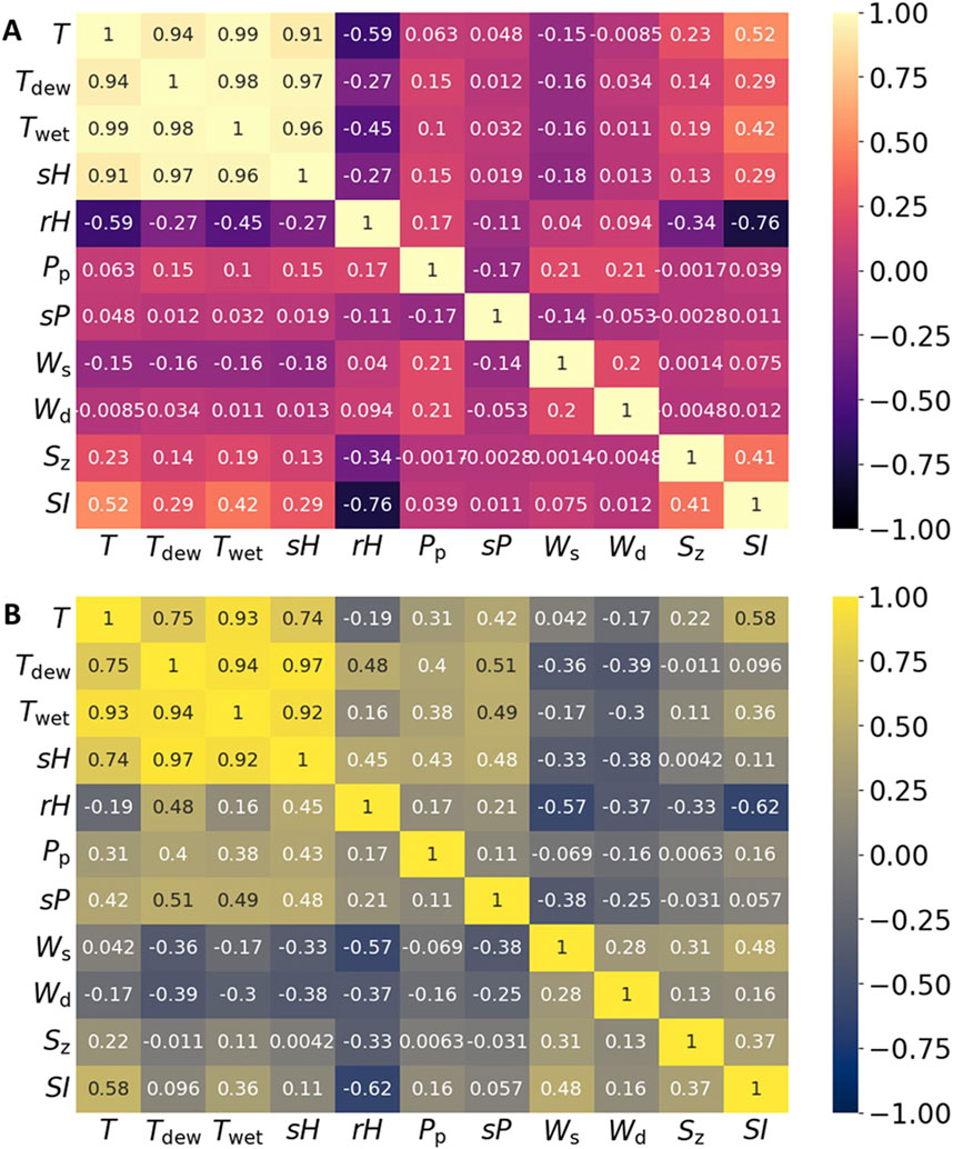
Figure 1. Heatmap illustrating the correlations between weather features and SI: (A) Munich, (B) Texas.

In Figure 1B, sourced from Texas, the data shown illustrates the $r_{vw}$ between eleven meteorological parameters and SI values. It is worth noting that T exhibits a moderate correlation (0.58) with SI, while T_wet shows a lower correlation (0.36). Conversely, rH and SI demonstrate notably strong negative correlations (−0.61). Furthermore, W_s displays a moderate correlation (0.48) with SI, whereas Sz demonstrates a low correlation (0.37). As a result, T, T_wet, rH, W_s, and S_z are identified as the primary inputs for the model, selected based on their $r_{vw}$. Table 1 presents a summary of the main characteristics of the two datasets. The chosen parameters provide a balanced and comprehensive input set for accurate modeling, reflecting both strong and moderate influences on SI. High-dimensional datasets often contain redundant features, which can complicate model training and degrade performance. The strength and direction of their correlations with SI help prioritize these parameters for inclusion in forecasting SI.

Table 1

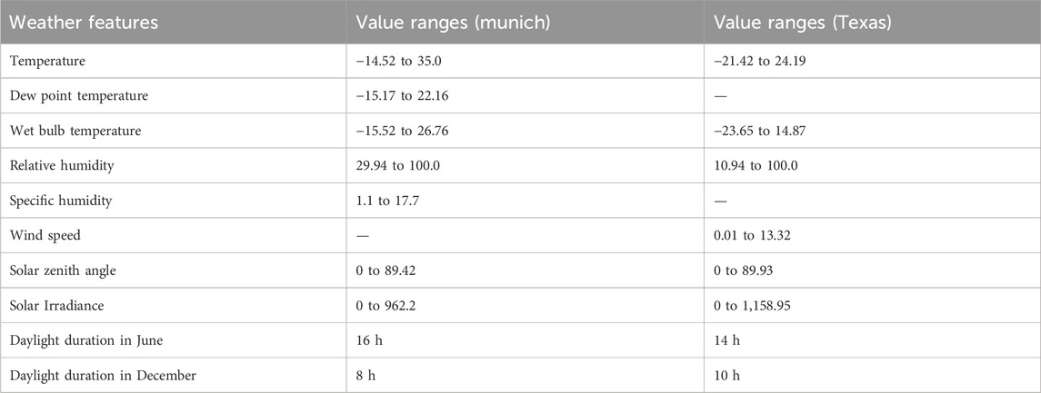
Table 1. Summary of the dataset and input feature selection using Pearson correlation analysis.

2.2.3 Data normalization

To normalize data, values measured on different scales are converted to a common scale, typically between 0 and 1, while maintaining the original range of value disparities. The Min-Max scaler employs the following formula to adjust features so that they lie within a specified range, typically 0 to 1 as defined in Equation 2 (Patro et al., 2015):

$X_s=\frac{X-X_{\mathit{min}}}{X_{\mathit{max}}-X_{\mathit{min}}}(2)$

Here $X_s$ is the scaled value of the original $X$, while $X_{\mathit{min}}$ and $X_{\mathit{max}}$ stand for the minimum and maximum values, respectively. The Min-Max Scaler ensure that all other values are proportionately scaled within this range, where the smallest value is mapped to 0 and its highest value is mapped to 1. This scaling method is beneficial when the data does not conform to a Gaussian distribution or when preserving the relative relationships among data points from the original dataset is important (Raju et al., 2020).

2.2.4 Re-integration of data column and target separation

After normalization of the numeric data, the date column is re-added to the scaled data frame to facilitate further analysis or date-based tracking. The target variable, assumed to be “SI,” is then separated from the predictors. This separation into X (features) and Y (target) is essential for supervised learning.

2.2.5 Data splitting

It’s crucial to divide the dataset into distinct training and validating subsets to fully evaluate the model’s performance. The training set is essential for model development, while the validating set offers an objective assessment of the model’s capacity for generalization. In this investigation, the data is split in an 80-20 ratio, with the larger portion used for training and the smaller portion for validation. These pre-processing steps are crucial to ensure that the data is properly formatted and of high quality, enabling effective training of a deep learning model to accurately predict SI. It is essential to assess whether the TIR model can effectively learn from the data and generate reliable, robust predictions.

3 Methodology

For the development and validation of the TIR model, we utilized a comprehensive suite of advanced Python libraries, including Matplotlib, Scikit-learn, TensorFlow, Keras, Seaborn, Pipeline, and Pandas (Xing et al., 2023). Data processing is performed using Google Collaboratory, a versatile platform that allows for Python code execution directly in the browser without setup requirements. Google Collaboratory provides free GPU access and facilitates easy sharing, making it an excellent resource for students, data scientists, and AI researchers.

3.1 Transformer-infused recurrent neural network (TIR) model

The TIR model leverages advanced neural network components specifically designed to capture temporal dependencies, thereby significantly enhancing the predictive accuracy of SI. This sophisticated architecture comprises multiple specialized layers, each meticulously crafted to execute distinct functions essential for time series forecasting (Hanif and Mi 2024). As illustrated in Figure 2, the TIR model incorporates a transformer component to boost performance, along with a BiLSTM encoder and a GRU decoder, ensuring a robust and efficient forecast of SI.

Figure 2

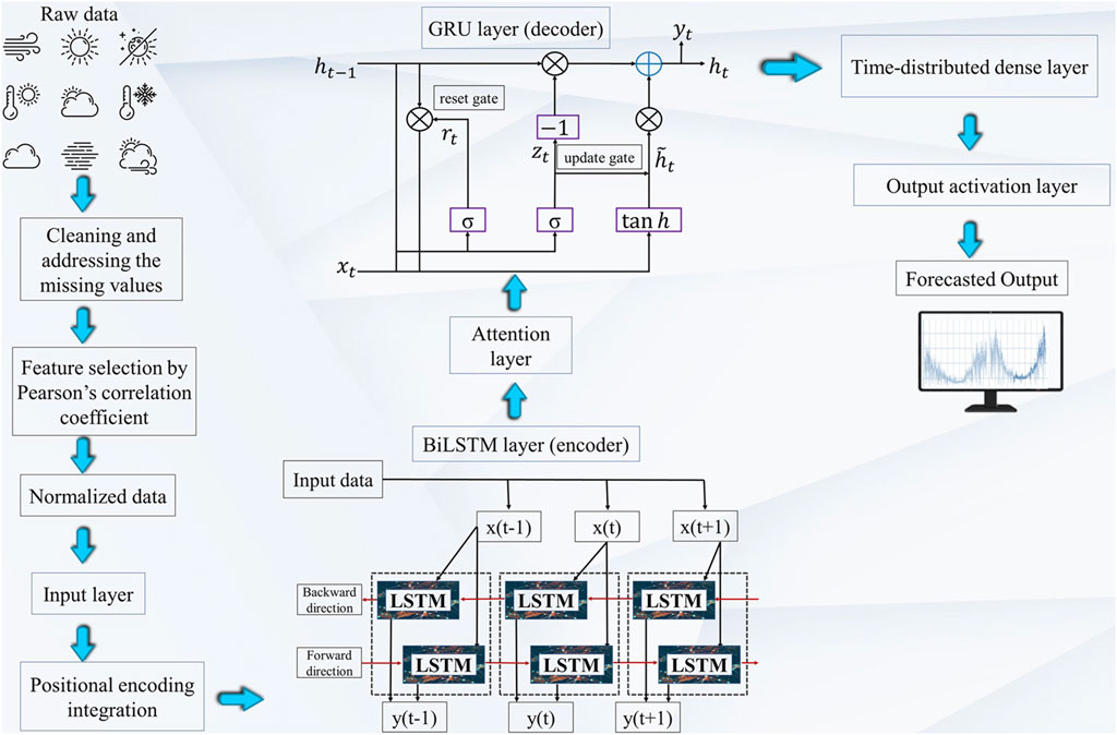
Figure 2. Structure of the TIR model.

3.1.1 Positional encoding integration

The TIR model integrates positional encoding into the input layer to capture the relative positions of time steps, which is essential for accurate SI forecasting (Zhu et al., 2022). SI data is inherently sequential, meaning the sequence of observations over time significantly impacts the prediction of future values (Ma et al., 2023; Gu et al., 2024). By incorporating positional encoding, the model generates fixed-dimensional representations for each time step, allowing it to distinguish between various temporal positions (Kong et al., 2023).

This capability enables the model to understand the temporal context of the data, recognizing patterns associated with daily and hourly changes in SI. As a result, the model can make more accurate predictions by considering the fluctuations in SI over time (Yan et al., 2020). Additionally, positional encoding helps the TIR model capture long-term dependencies, which are crucial for accurate SI predictions over extended periods. Consequently, the inclusion of positional encoding enhances the model’s ability to interpret and forecast complex time series data with precision. The positional encoding is calculated by using sine and cosine functions with varying frequencies from Equations 3, 4.

$EN{P}_{i,2j}=\mathit{sin}\left(\frac{i}{{10000}^{2j∕d}}\right),2_j\le d(3)$

$EN{P}_{i,2j+1}=\mathit{cos}\left(\frac{i}{{10000}^{2j∕d}}\right),2_{j+1}\le d(4)$

Here, the term $\frac{i}{{10000}^{2j∕d}}$ denotes the positional index for each embedding within the sequence, where $i,j$ and $d$ correspond to the embedding’s position in the sequence, the embedding’s dimension, and the model’s dimension, respectively.

3.1.2 Bi-directional LSTM layer (encoder)

In the TIR model, the Bi-directional LSTM layer functions as the encoder, playing a crucial role in forecasting SI. This Bi-directional approach is particularly advantageous for SI prediction as it enables the model to capture both past and future context surrounding each time step (Srivastava and Lessmann 2018; Ghimire et al., 2019; Husein and Chung 2019). Traditional DL techniques often struggle with accurately modeling temporal dependencies in time-series data due to their limited capacity to remember long-term patterns (Qing and Niu 2018). RNNs offer a short-term memory capability through their iterative processes within hidden layers, but they face challenges with long-term memory retention due to issues like gradient vanishing and explosion. To address these issues, the LSTM architecture is developed. Unlike traditional RNN, LSTM incorporate specialized memory cells and gating mechanisms (input, output, and forget gates) to regulate and preserve information over longer sequences (Wang et al., 2020b). This gating mechanism helps the LSTM maintain both short-term and long-term dependencies effectively (Zhou and Chen 2021). In the context of forecasting SI, the LSTM’s ability to manage these long-term dependencies is crucial, as SI patterns can span extended periods and are influenced by a variety of factors over time. By leveraging the Bi-directional LSTM architecture, the TIR model can more accurately forecast SI by integrating comprehensive temporal information and addressing the limitations of gradient vanishing and explosion inherent in simpler RNN structures. It consists of three fundamental elements: gates and cell memory states and can be mathematically defined in Equations 5–9.

$f_t=\sigma \left(w_{fg}\left[h_{t-1},x_t\right]+b_{fg}\right)(5)$

$i_t=\sigma \left(w_{in}\left[h_{t-1},x_t\right]+b_{in}\right)(6)$

$\stackrel{\sim }{c}=\sigma \left(w_{out}\left[h_{t-1},x_t\right]+b_{out}\right)(7)$

$c_t=f_t{c}_{t-1}+i_t\mathit{tanh}\left(w_{cell}\left[h_{t-1},x_t\right]+b_{cell}\right)(8)$

$h_t=\stackrel{\sim }{c}\mathit{tanh}\left(c_t\right)(9)$

In the above relations, weighted matrices are represented by $w_{fg}$, $w_{in}$, and $w_{out}$, while cell biases are represented by $b_{fg}$, $b_{in}$, and $b_{out}$. The input is denoted as $x_t$ and the hidden state vector as $h_t$. In the LSTM model, inputs are processed sequentially, and only previous inputs affect the current output. To overcome this one-way dependency, the BiLSTM architecture is explored. This architecture considers both past and future values by utilizing a duplicated LSTM structure that handles both forward and reverse time sequences (Gers et al., 2000). Consequently, by undergoing dual training iterations, the model can incorporate additional data characteristics. The architecture and hyperparameters of the BiLSTM model are detailed in Table 2. The output of the hidden layer, $h_t$ at the time step $t$ in the BiLSTM framework is defined as Equation 10 follows:

$h_t=\left[F{h}_t+B{h}_t\right](10)$

where $F{h}_t$ and $B{h}_t$ are represent forward and backward hidden sequences. Figure 2 illustrates the architectural blueprint of BiLSTM developed for SI prediction. The input is represented as $x\left(T\right)$, while the resulting output is represented as $y\left(T\right)$.

Table 2

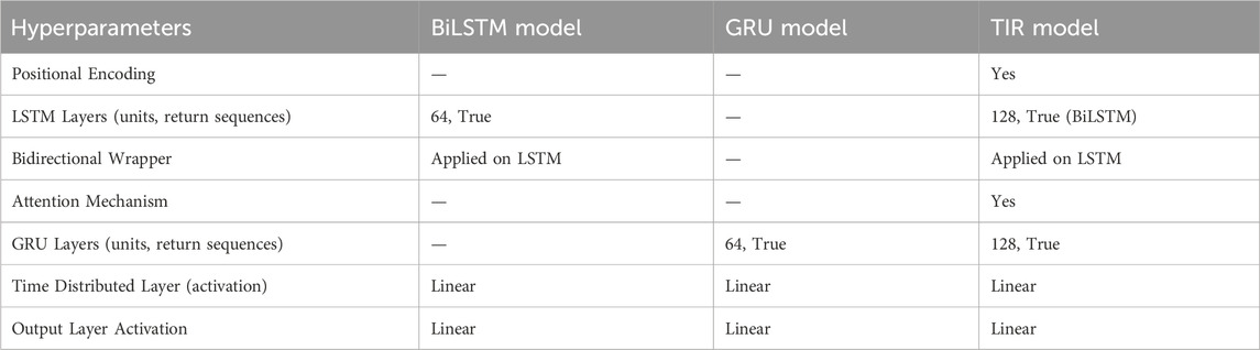
Table 2. Hyperparameters of the TIR model.

3.1.3 Attention mechanism layer

The attention mechanism is used on the output of the BiLSTM layer to help the model focus on specific parts of the input sequence, like different levels of SI, when making predictions. By combining the encoder outputs with weights, attention highlights important time steps related to SI patterns and enhances the model’s capacity to capture significant variations in the solar energy data (Brahma et al., 2021).

The expression of the attention mechanism is represented as Equations 11–13:

$d_{ij}=score\left(h_i,s_{j-1}\right)(11)$

${\alpha }_{ij}=\frac{\mathit{exp}\left(d_{ij}\right)}{{\sum }_{j=1}^{V_x}\mathit{exp}\left(d_{ik}\right)}(12)$

$c_i={\displaystyle \sum _{j=1}^{V_x}}{d}_{ij}{h}_i(13)$

Where $d_{ij}$ represent the attention score, ${\alpha }_{ij}$ denotes the attention weight, and $c_i$ is the context vector. This mechanism enables the model to dynamically adjust its focus according to the input sequence.

3.1.4 GRU layer (decoder)

The GRU layer is chosen as the decoder for forecasting SI due to its efficient handling of sequential data and streamlined architecture. Unlike LSTM networks, which have a more complex structure with multiple gates, the GRU uses only two gates (the update and reset gates) resulting in fewer parameters and reduced computational overhead (Elizabeth et al., 2022). This simplicity enhances the GRU’s capability to manage long-term dependencies while speeding up training times (Jaihuni et al., 2020; Zhong et al., 2021). In SI forecasting, the update gate is crucial as it controls how much historical data is retained, allowing the model to capture persistent trends in SI levels. Higher values in the update gate indicate greater retention of past data, which is essential for accurate predictions (Mahjoub et al., 2022). Conversely, the reset gate enables the GRU to focus on more recent, relevant data by disregarding less pertinent past information. This dynamic adjustment makes the GRU well-suited for the fluctuating nature of SI, balancing efficiency and effectiveness in predictive performance (Sajjad et al., 2020). Detailed in Figure 2, the complex architecture of the GRU is outlined. The forward propagation formula for the GRU network is expressed as Equations 14–17 follows:

$r_t=\sigma \left(U^r{x}_t+V^r{h}_{t-1}\right)(14)$

$z_t=\sigma \left(U^z{x}_t+V^z{h}_{t-1}\right)(15)$

${\stackrel{\sim }{h}}_t=\mathit{tanh}\left(r_{t}U{h}_{t-1}+V{x}_t\right)(16)$

$h_t=\left(1-z_t\right)h_{t-1}+z_t{\stackrel{\sim }{h}}_t(17)$

In the realm of neural network dynamics, $r_t$ and $z_t$ symbolize the outcomes of the reset gate and the update gate correspondingly. The variable $x_t$ signifies the input to the network at time $t$, while ht and $h_{t-1}$ represent the hidden state of the current node and the preceding hidden layer state at time $t-1$, sequentially. The term ${\stackrel{\sim }{h}}_t$ denotes the computational process involved in generating the candidate set from input $x_t$ and the output $h_{t-1}$. Notably, $\sigma$ and $\mathit{tanh}$ signify the sigmoid function and the hyperbolic tangent activation function, correspondingly. The weight matrices, delineated as $U^r$, $V^r$, $U^z$, $V^z$, $U$, and $V$, are pivotal components influencing the network’s dynamical behaviour. The architecture and hyperparameters of the GRU model are detailed in Table 2.

3.1.5 Time distributed dense layer

Lastly, to create predictions at each time step, a time distributed dense layer is applied to the GRU’s output. Forecasting SI at each time point in the time series depends on this layer’s ability to guarantee that each time step in the sequence has a unique output (Yang et al., 2020).

The dense layer that is time distributed can be explained as Equation 18 follows:

$y_t=dense\left(h_t\right)(18)$

In this context, $h_t$ represents the hidden state from the GRU at time step $t$ and $y_t$ is the corresponding output. A linear activation function is utilized to forecast the continuous values of SI. This approach treats each timestep as a distinct entity during forecasting tasks, such as predicting hourly SI. The output of this layer, typically continuous values generated with a linear activation function, represents the predicted target variable for each timestep. By analyzing each timestep separately, the time-distributed dense layer ensures that the model aligns its predictions with the temporal characteristics of the input data sequence.

3.1.6 Output activation layer

In a TIR framework utilized for SI prediction, the concluding activation layer is generally constituted as a linear layer. This terminal layer yields continuous outcomes by executing a linear transformation upon the outputs derived from the antecedent layers. Consequently, the model’s predictions manifest as a direct weighted aggregation of the features discerned by the network, thereby facilitating the generation of exact SI forecasts devoid of non-linearities. This uncomplicated methodology guarantees that the predicted values exhibit a continuous range, aligning seamlessly with the spectrum of anticipated SI measurements (Gao et al., 2022).

The TIR model’s architecture, detailed in Table 2, integrates positional encoding, attention mechanisms, GRU decoding, a time-distributed dense layer and output activation layer. These components collectively enhance the accuracy and effectiveness of SI forecasting hourly sequence time series data, particularly valuable in fields such as weather forecasting. Each component plays a crucial role in capturing and leveraging temporal dependencies, thereby improving forecast precision.

3.2 Evaluation metrics for assessing model performance

Metrics for performance evaluation are essential for assessing the DL model’s effectiveness. These measures enable comparisons and determine the model’s correctness. The primary method of assessing overall performance involves comparing the actual SI with the forecasted values (Wang et al., 2018). Specific metrics offer feedback on the accuracy of the forecasts, thereby aiding in the enhancement of precision. A lower score on these metrics signifies more accurate forecasting and serves as a guide to refine the models. Below, detailed mathematical formulations for the statistical metrics mentioned in Coefficient of Determination (R²), Root Mean Squared Error (RMSE), Mean Absolute Error (MAE), and Mean Squared Error (MSE), provided in Equations 19–22, offer a precise computational framework (Despotovic et al., 2015).

$R^2=1-\frac{{\displaystyle \sum _{i=1}^N}{\left(x_i-{\widehat{x}}_i\right)}^2}{{\displaystyle \sum _{i=1}^N}{\left(x_i-{\overline{x}}_i\right)}^2}(19)$

$RMSE=\sqrt{\frac{1}{N}{\displaystyle \sum _{i=1}^N}{\left(x_i-{\widehat{x}}_i\right)}^2}(20)$

$MAE=\frac{1}{N}{\displaystyle \sum _{i=1}^N}\left|x_i-{\widehat{x}}_i\right|(21)$

$MSE=\frac{1}{N}{\displaystyle \sum _{i=1}^N}{\left(x_i-{\widehat{x}}_i\right)}^2(22)$

In Equations 19–22, the variables $x_i$, ${\widehat{x}}_i$, ${\overline{x}}_i$, and N represent the ground truth values, predicted values, mean ground truth values of solar irradiance, and the number of observations, respectively. The attainment of elevated R² values is sought-after, as proximity to unity denotes superior model efficacy, reflecting a robust alignment of the regression line with the dataset. Conversely, a diminution in the values of RMSE signifies an improvement in model performance.

4 Results and discussion

In this section, the performance of TIR is rigorously tested, with a focus on its accuracy in identifying complex patterns within large datasets. Additionally, a benchmarking study is conducted to compare TIR against five other leading models, highlighting its superior capabilities.

4.1 Loss trends in TIR training and validation

The dataset is divided into training and validation subsets, with the training set comprising 80% of the total data. The model’s performance, evaluated using MSE, is monitored over 50 epochs. Figures 3A, B illustrate the training loss MSE for Munich and Texas, respectively. In Figure 3A, the validation loss for Munich shows a significant decrease during the initial 9 epochs, demonstrating the model’s ability to quickly learn and adapt. This rapid reduction suggests an efficient optimization process, leading to a stable low loss and indicating that the model has effectively captured the essential data patterns. The close alignment between the training and validation losses reflects the model’s robustness, with minimal overfitting, ensuring reliable performance on new data.

Figure 3

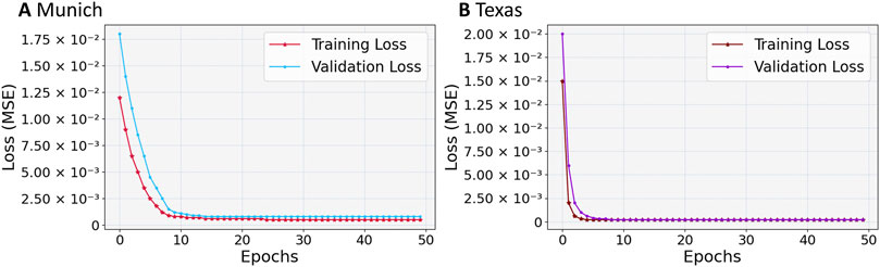
Figure 3. Training and validation loss (MSE) convergence curve for the TIR model across ephochs: (A) Munich, (B) Texas.

Figure 3B depicts the training process for the Texas dataset. The initial high losses drop significantly by epoch 5, highlighting the model’s quick learning capabilities. After epoch 5, the training and validation losses stabilize at low values, remaining close to each other, which underscores the model’s strong generalization skills. The consistently low loss values throughout the epochs indicate that the TIR model performs well across various datasets. This is further supported by its low final training and validation losses, which suggest high accuracy and dependability. The model’s ability to achieve minimal convergence of loss values points to an optimal solution, highlighting its effectiveness and precision. The steady and similar loss curves across different datasets demonstrate the TIR model’s adaptability and robustness, making it suitable for diverse applications. Additionally, the alignment of training and validation loss graphs confirms the model’s proficiency in fitting and predicting SI, showcasing its robustness and versatility in forecasting across different regions.

4.2 Assessing the TIR model

When the TIR model is utilized for SI forecasting in the intricate datasets of Munich and Texas, it demonstrates notable predictive efficacy, although with discrepancies indicative of regional SI patterns. Figure 4 displays the KDE for actual and predicted SI (Wh/m²) values in Munich and Texas. These estimations are generated using the TIR model. KDE is a non-parametric method for calculating a continuous variable’s probability density function. It produces a smooth curve that accurately represents the data distribution. This method allows for a meaningful comparison between actual and forecasted SI (Wh/m²) measurements, showcasing the model’s ability to capture underlying patterns in different geographic contexts. The KDE plots for Munich and Texas demonstrate the alignment between the actual and predicted values, indicating the model’s robustness and generalization capabilities. By analyzing the KDE curves, areas where the model performs well and potential discrepancies can be identified. This analysis is crucial for understanding spatial variability in SI predictions and improving the model’s accuracy in various environmental conditions (Chen 2017).

Figure 4

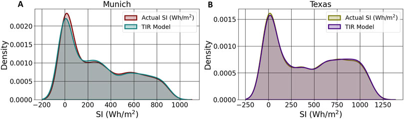
Figure 4. KDE plot of TIR prediction: (A) Munich, (B) Texas.

In Munich, the model’s density plot Figure 4A exhibits a distinct peak at SI ≈ 25 Wh/m², demonstrating the model’s precision in capturing the median irradiance values. Although some deviations are observed, these remain within an acceptable range, underscoring the model’s proficiency in handling the region’s SI variability. Conversely, in Texas, the density plot Figure 4B displays a peak at SI ≈ 11.6 Wh/m², indicating a high probability of this actual SI value. The predicted values are in good agreement with the actual SI values, showing little deviation and a large kernel density overlap.

The alignment of the curves in each graph powerfully demonstrates the model’s predictive precision. In Munich and Texas alike, the close correspondence between actual and forecasted data highlights the TIR model’s exceptional forecasting ability, despite varying weather conditions and input factors. The KDE curves reveal prominent peaks that indicate the most probable SI values, with both regions showing similar peak magnitudes.

The solar potential in cities like Brussels, Vienna (Nematchoua et al., 2022), Warsaw (Ronkiewicz et al., 2021), and Zurich (Srivastava and Lessmann 2018) has been well-documented, with many researchers evaluating their suitability for SE harvesting. The regions are characterized by a moderate to high level of SI, making them ideal candidates for validating solar forecasting models. Several studies have highlighted the significant SE potential of these areas, affirming their importance in solar energy research.

To further assess the generalizability of the TIR model, it was applied to forecast SI across these four cities. The evaluation metrics, including R², RMSE, MAE, and MSE, for each location, are presented in Table 3. The high R² values, ranging from 0.885 to 0.914, indicate that the TIR model captures a substantial proportion of the variance in SI across these regions. Notably, Zurich and Vienna exhibited the highest predictive accuracy, with R² values of 0.914 and 0.912, respectively. This suggests a strong correlation between the actual and predicted SI in these cities, underscoring the model’s robustness in diverse geographic settings.

Table 3

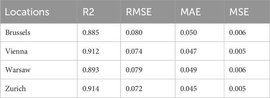
Table 3. Performance evaluation of the TIR model across multiple locations for generalization and robustness testing.

The RMSE values, ranging from 0.072 to 0.080, further confirm the model’s accuracy, with Zurich demonstrating the lowest error (0.072), followed closely by Vienna (0.074). These results indicate the model’s ability to predict SI with minimal deviation from the observed values, reinforcing its reliability. Similarly, the MAE values across all four cities remain within a narrow range (0.045–0.050), highlighting the model’s consistency in minimizing the absolute errors in SI predictions.

In terms of MSE, the values are notably low, with Zurich and Vienna once again performing the best (MSE = 0.005), followed by Brussels and Warsaw (MSE = 0.006). These findings reflect the TIR model’s capability to maintain high predictive accuracy across different environmental conditions, further validating its applicability beyond the initial regions of Munich and Texas.

Table 3 illustrates the generalizability of the TIR model and its proficiency in forecasting SI across a wider range of geographical locations, reaffirming its effectiveness as a reliable tool for solar energy predictions in diverse urban settings.

4.3 Performance comparison with state-of-the-art algorithms

This analysis undertakes a thorough evaluative comparison of various DL models for predicting SI. The performance of the TIR model is assessed against a suite of five distinct algorithms previously suggested by researchers. The models in question encompass a range of methodologies, including ANN, BiLSTM, GRU, transformers, and a hybrid BiLSTM-GRU model. Each algorithm has been subjected to a rigorous examination regarding its effectiveness and precision in forecasting SI. These specific adjustments are imperative to ensure that the evaluation remains equitable and pertinent to the unique attributes of the Munich and Texas datasets, as well as the research’s particular objectives. The hyperparameters of these comparative models are presented in Table 4.

Table 4

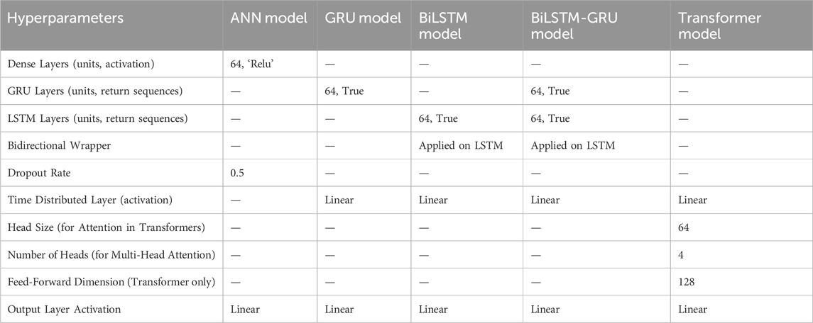
Table 4. Hyperparameters of the baseline models.

The intent behind these modifications is to enable a clear and unbiased comparison of the TIR model’s performance against established models in the field. The efficacy and appropriateness of the TIR model for SI prediction are depicted in Figures 5, 6.

Figure 5

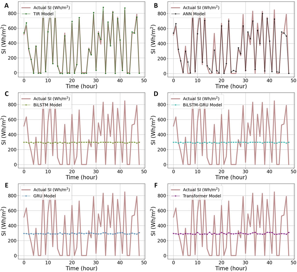
Figure 5. Comparison of the TIR and baseline models in Munich: (A) TIR, (B) ANN, (C) BiLSTM, (D) BiLSTM-GRU, (E) GRU, (F) Transformer.

Figure 6

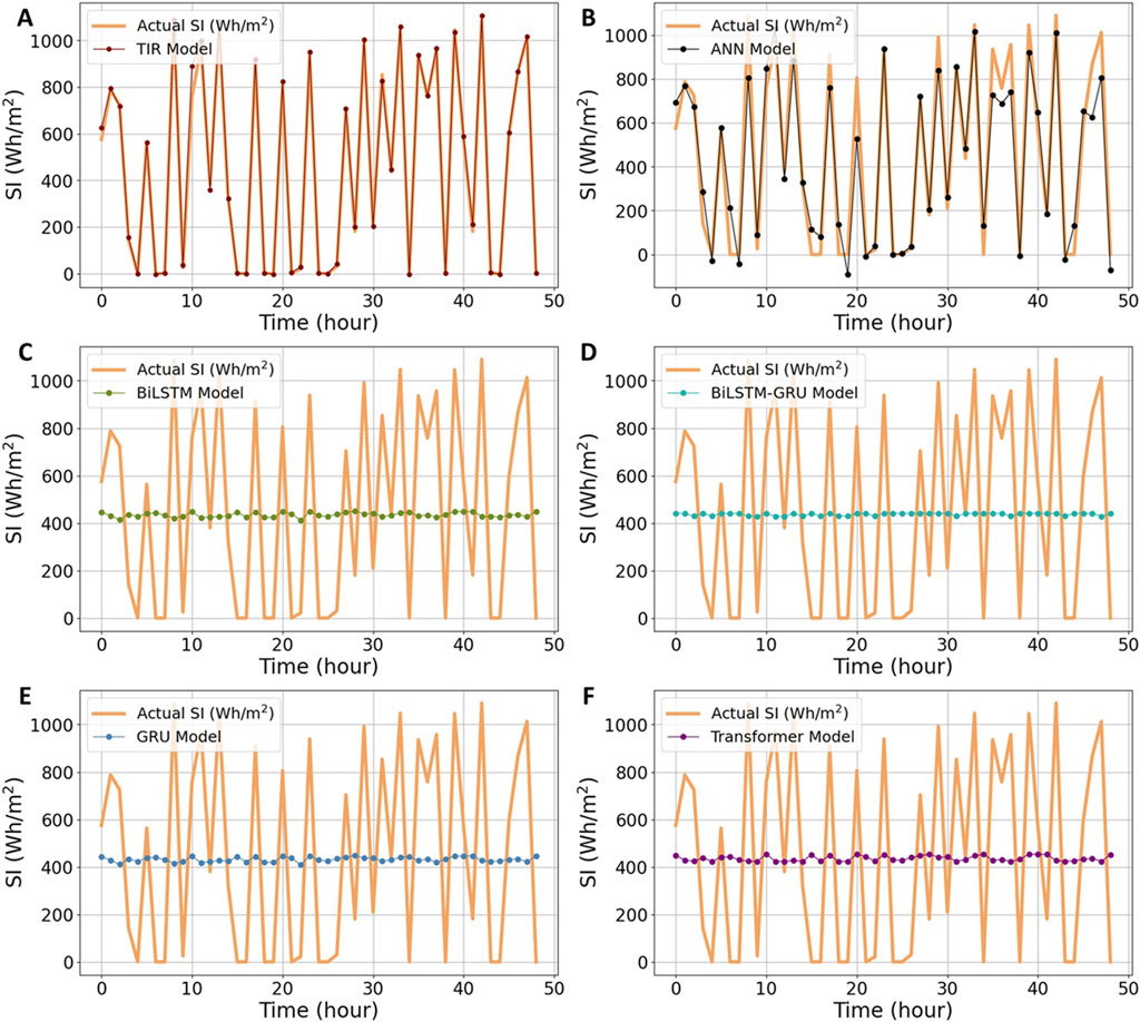
Figure 6. Comparisons of the TIR and baseline models in Texas: (A) TIR, (B) ANN, (C) BiLSTM, (D) BiLSTM-GRU, (E) GRU, (F) Transformer.

Upon analyzing the line graph Figure 5, several trends and patterns emerge. In Figure 5A, the TIR model unswervingly prevails over the other models over time, achieving a precision exceeding 97% by the end of the period. In contrast, the performance of the ANN model demonstrates considerable variability over time, characterized by fluctuations in accuracy and several abrupt declines, as illustrated in Figure 5B. Upon scrutinizing the Munich dataset, it becomes evident that the ANN model achieves remarkable accuracy, with an RMSE of 80.06, as depicted in Figure 5B. Conversely, the BiLSTM-GRU model records the highest error, with an RMSE of 280.9, as shown in Figure 5D, with detailed metrics provided in Table 5.

Table 5

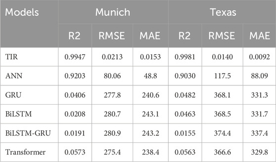
Table 5. Model comparison statistics.

Examining the GRU, BiLSTM, and transformer models, their respective RMSE values 277.8, 280.7, and 275.4, are considerably high and approximate the BiLSTM-GRU model’s performance. These values underscore the inadequate performance of these models on the Munich dataset. This pattern is consistent across RMSE and MAE values, although the TIR model emerges as a close contender. The R² scores, however, are especially remarkable, demonstrating a significant alignment with actual SI values at 0.9947, thus validating the model’s dependability and strength. In Figures 5C–F, the standalone DL models failed to effectively manage data outliers and thus did not achieve satisfactory results. In contrast, the TIR model demonstrated superior performance, effectively handling outliers and delivering significantly better outcomes.

Moving forward, Figure 6A illustrates the result of the perfect fitting achieved between the actual and predicted SI values in Texas. The TIR model demonstrates a nearly flawless alignment with minimal error, significantly outperforming other baseline models and exhibiting superior performance compared to the Munich region. In contrast, Figure 6B reveals a more pronounced discrepancy between the ANN model’s predictions and actual SI values, though this deviation remains within acceptable limits. It is also noteworthy that while the ANN model performs considerably better in Munich, it still falls short of the accuracy provided by the TIR model. Despite the GRU, BiLSTM, hybrid BiLSTM-GRU, and transformer models displaying augmented MSE and RMSE statistics, their R² coefficients of 0.0482, 0.0463, 0.0155, and 0.0563, respectively, as illustrated in Table 5, do not irrefutably suggest superior predictive efficacy. Figures 6C–F further depict the results from all baseline models, which show significantly poorer performance. The underperformance of these models can be attributed to the inherent complexity of the Texas datasets, which might include diverse and multifaceted patterns that these models are unable to capture effectively. Furthermore, the Texas datasets might possess unique domain-specific characteristics and intricate temporal and spatial dynamics that these models struggle to handle. In contrast, the TIR model demonstrates an enhanced ability to manage this complexity and predict the SI more accurately, indicating its superior capability to capture the nuanced patterns within the Texas datasets.

However, it shows a tendency to recover towards the end of the period in the Munich region compared to the Texas region. Furthermore, single recurrent and transformer models generally exhibit poorer performance, with high fluctuation rates in both regions. For instance, its hybrid structure might offer greater capacity or improved capability in handling the dataset’s complexity. However, in this case, the BiLSTM-GRU model does not fully capture the data for SI forecasting, as illustrated in Figures 5D, 6D. Based on the comprehensive evaluation, it can be concluded that the TIR model achieves higher prediction accuracy and significantly lower bias compared to other models in both regions.

4.4 Computational cost and efficiency

A detailed assessment of the computational efficiency and cost of the proposed TIR model compared to other models is provided. Table 6 summarizes key performance metrics, including total training time, inference time, model size, memory usage, and total trainable parameters. Although the TIR model demonstrates longer training times, its overall efficiency and predictive performance make it a compelling choice for SI forecasting, particularly in complex environments.

Table 6

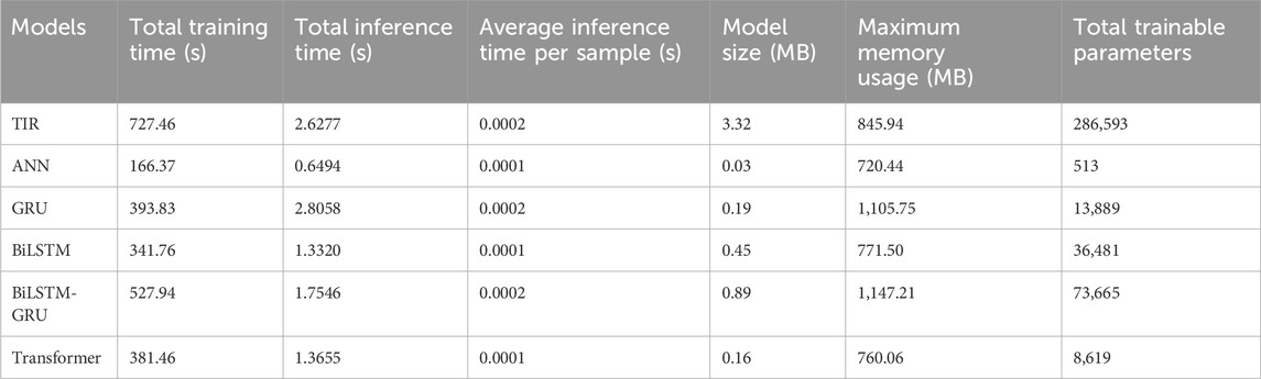
Table 6. Key performance metrics of the TIR and baseline models.

The TIR model’s extended training time of 727.46 s, while longer than other models such as ANN (166.37 s) and GRU (393.83 s), is justified by its superior ability to capture complex temporal dependencies and patterns inherent in SI data. This complexity is reflected in its larger model size (3.32 MB) and higher number of trainable parameters (286,593), which enable it to detect subtle and intricate relationships that simpler models may overlook. For instance, despite the faster training times of ANN and BiLSTM, their simpler architectures may struggle to achieve the same level of predictive accuracy, especially in datasets with significant variability like those of Munich and Texas. The ability of the TIR model to manage these intricacies demonstrates its robustness in handling highly complex datasets. Figure 7 vividly captures the training and inference durations of various DL models, highlighting significant disparities in computational efficiency.

Figure 7

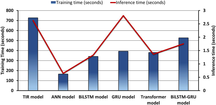
Figure 7. Time efficiency analysis of DL models during training and inference phase.

When compared to traditional models, such as ANN and GRU, the TIR model offers a more comprehensive representation of the underlying dynamics in the SI data, which translates into higher accuracy. The shorter training times of ANN and BiLSTM, while beneficial in reducing computational cost, come at the expense of model generalization. In contrast, the TIR model, though slower to train, offers superior predictive precision, as evidenced by its lower inference time per sample (0.0002 s), indicating that the model is efficient once deployed. Additionally, the TIR model’s memory usage (845.94 MB) remains moderate compared to GRU (1,105.75 MB) and BiLSTM-GRU (1,147.21 MB), highlighting its resource efficiency despite its deeper architecture.

The results of our study show that the TIR model generalizes well across different geographical and climate zones, despite its extended training time. In inference, the TIR model exhibits low total inference time (2.6277 s), on par with other models such as GRU (2.8058 s) and BiLSTM (1.3320 s). This suggests that while the model requires more time during the training phase, its inference efficiency makes it suitable for real-time applications where speed is critical once the model is fully trained.

4.4.1 Benefits of extended training time for the TIR model

The TIR, which combines the advantages of both transformers and RNNs, has emerged as a viable paradigm in recent advances in neural network architecture. The performance and generalization of TIR models can be significantly enhanced by extending their training period. Longer training increases convergence, lowers the chance of overfitting, and gives the model a greater knowledge of complicated patterns. Furthermore, as will be discussed below, extended training provides the network with additional chances to optimize its parameters, which raises accuracy in tasks involving sequential data, such time-series forecasting and natural language interpretation.

1. Increased Predictive Accuracy: Extensive research demonstrates that deep learning models, including the TIR model, benefit from longer training durations, leading to higher predictive accuracy. This is particularly crucial for SI forecasting, where precision in capturing temporal dependencies directly influences energy optimization and grid stability.

2. Long-Term Stability and Performance: The TIR model, owing to its longer training time, shows enhanced stability and long-term performance, particularly in maintaining accuracy across multiple data samples. As overfitting is less likely, the model can better generalize to new data, providing consistent and reliable long-term forecasts.

3. Efficiency During Inference: Despite the longer training period, the TIR model’s inference time remains competitive. With an average inference time of just 0.0002 s per sample, the model proves to be effective during deployment. This efficiency is crucial for real-time solar forecasting systems, where fast response times are essential for optimizing energy generation and grid management.

4. Adaptability to Various Climate Conditions: The prolonged training phase of the TIR model allows for more thorough fine-tuning and parameter optimization. This enables the model to adapt more effectively to varying weather conditions and geographic regions, offering greater flexibility in different environmental scenarios.

Although the TIR model’s current training time is longer, advancements in training optimizations such as hardware acceleration and distributed computing offer opportunities to reduce these times without compromising performance. In addition, transfer learning techniques could be utilized to further decrease the model’s initial training time, allowing for quicker adaptation to new datasets or climate zones.

In summary, while the TIR model requires a more significant computational investment during training, its superior predictive accuracy, inference efficiency, and robustness make it a highly effective tool for SI forecasting in diverse environments. With ongoing research and technological advancements, the computational costs associated with DL models like TIR are expected to decrease, enhancing their applicability in real-time forecasting systems.

5 Strategic insights and analysis

This research represents a seminal contribution to the application of a TIR model in SI forecasting, highlighting the avant-garde amalgamation of diverse DL techniques to augment predictive precision. The discourse on the SI forecasting outcomes unequivocally demonstrates that the integration of a TIR framework markedly bolsters predictive proficiency. Employing the Pearson correlation coefficient for feature selection has discerned the most influential predictors for each locale, thereby enabling the construction of a model adept at discerning the nuanced impacts of various environmental factors on SI.

The TIR model, distinguished by its sophisticated deep recurrent network architecture, has exhibited remarkable accuracy across a diverse array of datasets, underscoring the efficacy of advanced deep learning techniques in SI forecasting. The model adeptly captures intricate environmental patterns, particularly in datasets where these patterns are pronounced. Its prowess in balancing complexity while averting overfitting has been integral to its outstanding performance. Figures 5, 6 provide compelling visual evidence of the superior predictive accuracy of both the TIR and ANN models, as illustrated by the results for the Texas and Munich datasets. Notably, the TIR model demonstrates a remarkable congruence between predicted and actual data points in both datasets. The thorough training and validation process highlight the model’s adeptness in assimilating knowledge from the training data and its capability to generalize this knowledge to novel, unseen data. This proficiency is especially evident from the consistent decline in loss values during the training phase and the stability of these values when assessed on the validation sets.

The superior performance of TIR can be attributed to its capacity to integrate the strengths of RNNs (BiLSTM acts as an encoder and GRU acts as a decoder) with the attention mechanism and positional encoding. This integration enables the model to capture intricate temporal dependencies and focus on the relevant parts of the input sequence, resulting in more precise predictions of SI. Munich and Texas present specific weather patterns, seasonal variations, and geographical features that complicate the prediction of SI. The advanced architecture of TIR is likely more adept at capturing these complex, localized patterns compared to other models. Models including ANN, BiLSTM, GRU, Transformers, and the hybrid BiLSTM-GRU architecture frequently encounter difficulties when addressing complex patterns in SI data. These challenges stem from several limitations such as susceptibility to overfitting or underfitting, suboptimal feature extraction, and complications in the training process and hyperparameter optimization. Although transformers are recognized for their robust capabilities, they demand substantial computational resources and may still encounter issues related to data quality and scalability. Moreover, the integration of diverse model architectures presents its own set of complexities, with problems like vanishing gradients or restricted contextual comprehension further impeding performance. Therefore, achieving superior outcomes necessitates a meticulous approach to model selection, balancing resource availability, and understanding data-specific characteristics.

The extensive appraisal augments the model’s veracity. When juxtaposed with both traditional and avant-garde forecasting methodologies, the TIR model consistently yielded more precise SI prognostications. This is corroborated by density and line graphs, where the TIR forecasts exhibit a close alignment with the reference trajectory, underscoring notable precision. Moreover, the model’s versatility and resilience across a spectrum of environmental scenarios not only authenticate its global applicability but also signify a significant leap in refining the utility and efficacy of SE prediction mechanisms.

Notwithstanding the model’s demonstrated abilities, it is critical to understand some of its intrinsic constraints. To make the model work in different climate zones, it might need to be modified. This is a chance to make it better and more unique, not a limitation. In addition, the intricacy of this sophisticated model presents computational difficulties that may exhaust available resources, specifically with regard to TIR. This research aims to optimize model parameters and automate feature selection through heuristic optimization methods. This foundational work sets the stage for future research to delve into exploring and evaluating various prediction intervals using advanced temporal techniques, thereby enhancing the robustness and applicability of predictive models.

These findings have significant implications for the field of SI forecasting. Precise SI predictions are crucial for effective SE management and seamless grid integration. The improved forecasting accuracy of the TIR model can result in more dependable energy production estimates, optimizing the operation of SE plants and enhancing the stability of power systems. Additionally, the model’s flexibility across various sites highlights its potential for worldwide application, which is essential in an increasingly interconnected and environmentally conscious world.

5.1 Limitations and future work

While this study yields promising results, it is essential to recognize its limitations and the opportunities they present for future research. One limitation is the model’s reliance on high-quality environmental data, which may not be available everywhere, potentially limiting its effectiveness in data-scarce areas. Additionally, incorporating additional data sources, such as real-time weather satellite imagery, could enhance predictions further. Future studies could also investigate the model’s scalability in real-world settings and its application to other renewable energy sources like wind or hydroelectric power. Addressing these limitations and exploring these future directions will advance renewable energy forecasting, enhancing global energy sustainability and reliability.

In order to boost its effectiveness and application, future research on the TIR model should concentrate on a number of important aspects. The existing model, while highly accurate, demands a large amount of computational power; hence, it is imperative to optimize training and inference timeframes. These timeframes could be reduced with techniques like parallel and distributed training employing cloud-based platforms or specialized hardware (such as TPUs and multi-GPU configurations). By moving information from the intricate TIR model to a more straightforward one and retaining accuracy during a shorter training period, knowledge distillation may also be helpful. Lastly, adding online and real-time learning capabilities could significantly improve the model’s adaptability in changing situations by enabling it to update continuously as new data is received without requiring a complete retraining.

6 Conclusion

This paper introduces the TIR model to address the challenges in forecasting SI caused by its stochastic nature. Data from Munich (Germany) and Texas (USA) are used to train and validate the TIR model. It integrates a BiLSTM model as the encoder and a GRU model as the decoder, enhanced by the attention mechanism and positional encoding, to improve the preservation of computational dependencies and reduce error terms compared to conventional recurrent models. To mitigate overfitting, data outliers, and complexity, the BiLSTM architecture is used for initial training, followed by the GRU as the decoder with attention mechanisms.

Key findings include:

• The TIR model showed outstanding precision in forecasting SI, notably excelling in the Texas dataset with an RMSE of 0.0140 and MAE of 0.0092. Although its performance in the Munich dataset slightly declined, yielding RMSE of 0.0213 and MAE of 0.0153, the model consistently demonstrated robust proficiency in capturing SI dynamics.

• The examination demonstrated the TIR model’s strengths in comparison to conventional DL algorithms such as ANN, BiLSTM, GRU, Transformer, and BiLSTM-GRU. In particular, ANN exhibited a slight performance advantage, achieving the highest R² value of 0.9203 in Munich, followed by TIR. This underscores their superior capability in managing intricate data interactions compared to BiLSTM, GRU, Transformer, and BiLSTM-GRU.

• Comprehensive case studies confirm the TIR model’s superiority in terms of lower error rates, higher accuracy, and reduced complexity when compared to other conventional DL models. The superiority of this model architecture may arise from the unique abilities of Transformers, such as attention mechanisms for capturing dependencies, and RNNs for sequential data processing, combined in a synergistic way within this model architecture.

In order to improve SE forecasts and maximize power-generating efficiency, a major development in SI forecasting has been made using the TIR model. To get around the drawbacks of the DL approach, future studies should look at novel predictive frameworks, like sophisticated reinforcement learning strategies. Real-time energy management, smooth integration of SE into smart grids, and improved strategic decision-making might all be facilitated by the development of an advanced hybrid SE prediction model. When preparing for upcoming SE projects, governments and investors would greatly benefit from this.

Data availability statement

Publicly available datasets were analyzed in this study. This data can be found here: The solar and meteorological datasets statement is available here: https://power.larc.nasa.gov/.

Author contributions

MSN: Conceptualization, Formal Analysis, Investigation, Methodology, Software, Visualization, Writing–original draft. MFH: Conceptualization, Formal Analysis, Investigation, Methodology, Software, Visualization, Writing–original draft, Supervision. MM: Validation, Writing–review and editing, Funding acquisition, Resources. II: Validation, Writing–review and editing, Software, Visualization. EL: Validation, Writing–review and editing, Data curation, Formal Analysis. XL: Validation, Writing–review and editing, Data curation, Methodology, Visualization. JM: Project administration, Resources, Supervision, Writing–review and editing.

Funding

The author(s) declare that financial support was received for the research, authorship, and/or publication of this article.

Acknowledgments

The authors would like to thank the Research Supporting Project number (RSP 2024R89), King Saud University, Riyadh, Saudi Arabia for funding this work.

Conflict of interest

The authors declare that the research was conducted in the absence of any commercial or financial relationships that could be construed as a potential conflict of interest.

Publisher’s note

All claims expressed in this article are solely those of the authors and do not necessarily represent those of their affiliated organizations, or those of the publisher, the editors and the reviewers. Any product that may be evaluated in this article, or claim that may be made by its manufacturer, is not guaranteed or endorsed by the publisher.

References

Ahlgren, P., Jarneving, B., and Rousseau, R. (2003). Requirements for a cocitation similarity measure, with special reference to Pearson’s correlation coefficient. J. Am. Soc. Inf. Sci. Technol. 54 (6), 550–560. doi:10.1002/asi.10242

CrossRef Full Text | Google Scholar

Al-Musaylh, M. S., Deo, R. C., Adamowski, J. F., and Li, Y. (2018). Short-term electricity demand forecasting with MARS, SVR and ARIMA models using aggregated demand data in Queensland, Australia. Adv. Eng. Inf. 35, 1–16. doi:10.1016/j.aei.2017.11.002

CrossRef Full Text | Google Scholar

Anuradha, K., Erlapally, D., Karuna, G., Srilakshmi, V., and Adilakshmi, K. (2021). “Analysis of solar power generation forecasting using machine learning techniques,” in E3S web of conferences.

CrossRef Full Text | Google Scholar

Armstrong, R. A. (2019) Should Pearson’s correlation coefficient be avoided? Ophthalmic Physiol. Opt. 39, 316, 327. doi:10.1111/opo.12636

PubMed Abstract | CrossRef Full Text | Google Scholar

Asmelash, E., and Gorini, R. (2021). International oil companies and the energy transition. Int. Renew. Energy Agency.

Google Scholar

Bandara, K., Shi, P., Bergmeir, C., Hewamalage, H., Tran, Q., and Seaman, B. (2019). “Sales demand forecast in E-commerce using a long short-term memory neural network methodology,” in Lecture notes in computer science (including subseries lecture notes in artificial intelligence and lecture notes in bioinformatics).

CrossRef Full Text | Google Scholar

Bouzgou, H., and Gueymard, C. A. (2017). Minimum redundancy – maximum relevance with extreme learning machines for global solar radiation forecasting: toward an optimized dimensionality reduction for solar time series. Sol. Energy 158, 595–609. doi:10.1016/j.solener.2017.10.035

CrossRef Full Text | Google Scholar

Brahma, B., Wadhvani, R., and Shukla, S. (2021). Attention mechanism for developing wind speed and solar irradiance forecasting models. Wind Eng. 45 (6), 1422–1432. doi:10.1177/0309524x20981885

CrossRef Full Text | Google Scholar

Chen, Y. C. (2017). A tutorial on kernel density estimation and recent advances. Biostat. Epidemiol. 1 (1), 161–187. doi:10.1080/24709360.2017.1396742

CrossRef Full Text | Google Scholar

Del Ser, J., Osaba, E., Sanchez-Medina, J., Fister, I., and Fister, I. (2020). Bioinspired computational intelligence and transportation systems: a long road ahead. IEEE Trans. Intelligent Transp. Syst. 21 (2), 466–495. doi:10.1109/tits.2019.2897377

CrossRef Full Text | Google Scholar

Despotovic, M., Nedic, V., Despotovic, D., and Cvetanovic, S. (2015). Review and statistical analysis of different global solar radiation sunshine models. Renew. Sustain. Energy Rev. 52, 1869–1880. doi:10.1016/j.rser.2015.08.035

CrossRef Full Text | Google Scholar

Elizabeth, M. N., Hasan, S., Al-Durra, A., and Mishra, M. (2022). Short-term solar irradiance forecasting based on a novel Bayesian optimized deep Long Short-Term Memory neural network. Appl. Energy 324, 119727. doi:10.1016/j.apenergy.2022.119727

CrossRef Full Text | Google Scholar

Farivar, G., and Asaei, B. (2011). A new approach for solar module temperature estimation using the simple diode model. IEEE Trans. Energy Convers. 26 (4), 1118–1126. doi:10.1109/tec.2011.2164799

CrossRef Full Text | Google Scholar

Gao, Y., Miyata, S., and Akashi, Y. (2022). Interpretable deep learning models for hourly solar radiation prediction based on graph neural network and attention. Appl. Energy 321, 119288. doi:10.1016/j.apenergy.2022.119288

CrossRef Full Text | Google Scholar

García-Hinde, O., Terrén-Serrano, G., Hombrados-Herrera, M., Gómez-Verdejo, V., Jiménez-Fernández, S., Casanova-Mateo, C., et al. (2018). Evaluation of dimensionality reduction methods applied to numerical weather models for solar radiation forecasting. Eng. Appl. Artif. Intell. 69, 157–167. doi:10.1016/j.engappai.2017.12.003

CrossRef Full Text | Google Scholar

Gers, F. A., Schmidhuber, J., and Cummins, F. (2000). Learning to forget: continual prediction with LSTM. Neural comput. 12 (10), 2451–2471. doi:10.1162/089976600300015015

PubMed Abstract | CrossRef Full Text | Google Scholar

Ghimire, S., Deo, R. C., Raj, N., and Mi, J. (2019). Deep solar radiation forecasting with convolutional neural network and long short-term memory network algorithms. Appl. Energy 253, 113541. doi:10.1016/j.apenergy.2019.113541

CrossRef Full Text | Google Scholar

Gu, Y., Hu, Z., Zhao, Y., Liao, J., and Zhang, W. (2024). MFGTN: a multi-modal fast gated transformer for identifying single trawl marine fishing vessel. Ocean. Eng., 303. doi:10.1016/j.oceaneng.2024.117711

CrossRef Full Text | Google Scholar

Gundu, V., Simon, S. P., and Kumba, K. (2024). Short-term solar power forecasting- an approach using JAYA based recurrent network model. Multimed. Tools Appl. 83 (11), 32411–32422. doi:10.1007/s11042-023-16723-w

CrossRef Full Text | Google Scholar

Hanif, M. F., and Mi, J. (2024). Harnessing AI for solar energy: emergence of transformer models. Appl. Energy 369, 123541. doi:10.1016/j.apenergy.2024.123541

CrossRef Full Text | Google Scholar

Hanif, M. F., Naveed, M. S., Metwaly, M., Si, J., Liu, X., and Mi, J. (2024a). Advancing solar energy forecasting with modified ANN and light GBM learning algorithms. AIMS Energy 12 (2), 350–386. doi:10.3934/energy.2024017

CrossRef Full Text | Google Scholar

Hanif, M. F., Siddique, M. U., Si, J., Naveed, M. S., Liu, X., and Mi, J. (2024b). Enhancing solar forecasting accuracy with sequential deep artificial neural network and hybrid random forest and gradient boosting models across varied terrains. Adv. Theory Simul. 7 (7). doi:10.1002/adts.202301289

CrossRef Full Text | Google Scholar

Husein, M., and Chung, I. Y. (2019). Day-ahead solar irradiance forecasting for microgrids using a long short-term memory recurrent neural network: a deep learning approach. Energies (Basel) 12 (10), 1856. doi:10.3390/en12101856

CrossRef Full Text | Google Scholar

Jaihuni, M., Basak, J. K., Khan, F., Okyere, F. G., Arulmozhi, E., Bhujel, A., et al. (2020). A partially amended hybrid Bi-Gru—ARIMA model (PAHM) for predicting solar irradiance in short and very-short terms. Energies (Basel) 13 (2), 435. doi:10.3390/en13020435

CrossRef Full Text | Google Scholar

Japkowicz, N. (2001). Supervised versus unsupervised binary-learning by feedforward neural networks. Mach. Learn 42 (1–2). doi:10.1023/A:1007660820062

CrossRef Full Text | Google Scholar

Jiang, Y. (2009). Computation of monthly mean daily global solar radiation in China using artificial neural networks and comparison with other empirical models. Energy 34 (9), 1276–1283. doi:10.1016/j.energy.2009.05.009

CrossRef Full Text | Google Scholar

Junninen, H., Niska, H., Tuppurainen, K., Ruuskanen, J., and Kolehmainen, M. (2004). Methods for imputation of missing values in air quality data sets. Atmos. Environ. 38 (18), 2895–2907. doi:10.1016/j.atmosenv.2004.02.026

CrossRef Full Text | Google Scholar

Kabir, E., Kumar, P., Kumar, S., Adelodun, A. A., and Kim, K. H. (2018). Solar energy: potential and future prospects. Renew. Sustain. Energy Rev. 82, 894–900. doi:10.1016/j.rser.2017.09.094

CrossRef Full Text | Google Scholar

Kawaguchi, K., Bengio, Y., and Kaelbling, L. (2022). “Generalization in deep learning,” in Mathematical aspects of deep learning.

CrossRef Full Text | Google Scholar

Khodayar, M., Kaynak, O., and Khodayar, M. E. (2017). Rough deep neural architecture for short-term wind speed forecasting. IEEE Trans. Ind. Inf. 13 (6), 2770–2779. doi:10.1109/tii.2017.2730846

CrossRef Full Text | Google Scholar

Khodayar, M., and Wang, J. (2019). Spatio-temporal graph deep neural network for short-term wind speed forecasting. IEEE Trans. Sustain Energy 10 (2), 670–681. doi:10.1109/tste.2018.2844102

CrossRef Full Text | Google Scholar

Kong, X., Du, X., Xue, G., and Xu, Z. (2023). Multi-step short-term solar radiation prediction based on empirical mode decomposition and gated recurrent unit optimized via an attention mechanism. Energy 282, 128825. doi:10.1016/j.energy.2023.128825

CrossRef Full Text | Google Scholar

Kumari, P., and Toshniwal, D. (2021). Deep learning models for solar irradiance forecasting: a comprehensive review. J. Clean. Prod. 318, 128566. doi:10.1016/j.jclepro.2021.128566

CrossRef Full Text | Google Scholar

Lauret, P., Voyant, C., Soubdhan, T., David, M., and Poggi, P. (2015). A benchmarking of machine learning techniques for solar radiation forecasting in an insular context. Sol. Energy 112, 446–457. doi:10.1016/j.solener.2014.12.014

CrossRef Full Text | Google Scholar

Liu, C. H., Gu, J. C., and Yang, M. T. (2021). A simplified LSTM neural networks for one day-ahead solar power forecasting. IEEE Access 9, 17174–17195. doi:10.1109/access.2021.3053638

CrossRef Full Text | Google Scholar

Liu, Y., Zhou, Y., Chen, Y., Wang, D., Wang, Y., and Zhu, Y. (2020). Comparison of support vector machine and copula-based nonlinear quantile regression for estimating the daily diffuse solar radiation: a case study in China. Renew. Energy 146, 1101–1112. doi:10.1016/j.renene.2019.07.053

CrossRef Full Text | Google Scholar

Ma, D., Fang, H., Wang, N., Lu, H., Matthews, J., and Zhang, C. (2023). Transformer-optimized generation, detection, and tracking network for images with drainage pipeline defects. Computer-Aided Civ. Infrastructure Eng. 38 (15), 2109–2127. doi:10.1111/mice.12970

CrossRef Full Text | Google Scholar

Ma, K., Yang, J., and Liu, P. (2020). Relaying-assisted communications for demand response in smart grid: cost modeling, game strategies, and algorithms. IEEE J. Sel. Areas Commun. 38 (1), 48–60. doi:10.1109/jsac.2019.2951972

CrossRef Full Text | Google Scholar

Mahjoub, S., Chrifi-Alaoui, L., Marhic, B., and Delahoche, L. (2022). Predicting energy consumption using LSTM, multi-layer GRU and drop-GRU neural networks. Sensors 22 (11), 4062. doi:10.3390/s22114062

PubMed Abstract | CrossRef Full Text | Google Scholar

Mele, M., Gurrieri, A. R., Morelli, G., and Magazzino, C. (2021). Nature and climate change effects on economic growth: an LSTM experiment on renewable energy resources. Environ. Sci. Pollut. Res. 28 (30), 41127–41134. doi:10.1007/s11356-021-13337-3

CrossRef Full Text | Google Scholar

Mellit, A., Pavan, A. M., and Lughi, V. (2021). Deep learning neural networks for short-term photovoltaic power forecasting. Renew. Energy 172, 276–288. doi:10.1016/j.renene.2021.02.166

CrossRef Full Text | Google Scholar

Nadeem, A., Hanif, M. F., Naveed, M. S., Hassan, M. T., Gul, M., Husnain, N., et al. (2024). AI-Driven precision in solar forecasting: breakthroughs in machine learning and deep learning. AIMS Geosci. Internet 10 (4), 684–734. doi:10.3934/geosci.2024035

CrossRef Full Text | Google Scholar

Nematchoua, M. K., Orosa, J. A., and Afaifia, M. (2022). Prediction of daily global solar radiation and air temperature using six machine learning algorithms; a case of 27 European countries. Ecol. Inf. 69, 101643. doi:10.1016/j.ecoinf.2022.101643

CrossRef Full Text | Google Scholar

Patro, S. G. K., and sahu, K. K. (2015). Normalization: a preprocessing stage. IARJSET, 20–22. doi:10.17148/iarjset.2015.2305

CrossRef Full Text | Google Scholar

Pawar, P., Mithulananthan, N., and Raza, M. Q. (2020). “Solar PV power forecasting using modified SVR with gauss-Newton method,” in Proceedings - 2020 IEEE 2nd global power, energy and communication conference, GPECOM 2020, 20–23 Oct, 2020.

CrossRef Full Text | Google Scholar

Pi, M., Jin, N., Chen, D., and Lou, B. (2022). Short-term solar irradiance prediction based on multichannel LSTM neural networks using edge-based IoT system. Wirel. Commun. Mob. Comput. 2022, 1–11. doi:10.1155/2022/2372748

CrossRef Full Text | Google Scholar

Qing, X., and Niu, Y. (2018). Hourly day-ahead solar irradiance prediction using weather forecasts by LSTM. Energy 148, 461–468. doi:10.1016/j.energy.2018.01.177

CrossRef Full Text | Google Scholar

Raju, V. N. G., Lakshmi, K. P., Jain, V. M., Kalidindi, A., and Padma, V. (2020). “Study the influence of normalization/transformation process on the accuracy of supervised classification,” in Proceedings of the 3rd international conference on smart systems and inventive technology, Tirunelveli, India, 20–22 August, 2020.

CrossRef Full Text | Google Scholar

Ronkiewicz, T., Aleksiejuk-Gawron, J., Awtoniuk, M., and Kurek, J. (2021). “Neural modelling of solar radiation variability,” in Journal of physics: conference series.

CrossRef Full Text | Google Scholar

Sajjad, M., Khan, Z. A., Ullah, A., Hussain, T., Ullah, W., Lee, M. Y., et al. (2020). A novel CNN-GRU-Based hybrid approach for short-term residential load forecasting. IEEE Access 8, 143759–143768. doi:10.1109/access.2020.3009537

CrossRef Full Text | Google Scholar

Salcedo-Sanz, S., Ghamisi, P., Piles, M., Werner, M., Cuadra, L., Moreno-Martínez, A., et al. (2020). Machine learning information fusion in Earth observation: a comprehensive review of methods, applications and data sources. Inf. Fusion 63, 256–272. doi:10.1016/j.inffus.2020.07.004

CrossRef Full Text | Google Scholar

Salehin, I., and Kang, D. K. (2023). A review on dropout regularization approaches for deep neural networks within the scholarly domain. Electron. Switz. 12, 3106. doi:10.3390/electronics12143106

CrossRef Full Text | Google Scholar

Sellaouti, A., Tiessler, M., Pobudzei, M., and Hoffmann, S. (2024). “Evolution and characteristics of shared e-scooters usage in Munich, Germany - results of an over 8 million trips data analysis,” in Transportation research procedia.

CrossRef Full Text | Google Scholar

Shadab, A., Said, S., and Ahmad, S. (2019). Box–Jenkins multiplicative ARIMA modeling for prediction of solar radiation: a case study. Int. J. Energy Water Resour. 3 (4), 305–318. doi:10.1007/s42108-019-00037-5

CrossRef Full Text | Google Scholar

Shahbaz, M., Topcu, B. A., Sarıgül, S. S., and Vo, X. V. (2021). The effect of financial development on renewable energy demand: the case of developing countries. Renew. Energy 178, 1370–1380. doi:10.1016/j.renene.2021.06.121

CrossRef Full Text | Google Scholar

Shakya, A., Michael, S., Saunders, C., Armstrong, D., Pandey, P., Chalise, S., et al. (2017). Solar irradiance forecasting in remote microgrids using Markov switching model. IEEE Trans. Sustain Energy 8 (3), 895–905. doi:10.1109/tste.2016.2629974

CrossRef Full Text | Google Scholar

Sher, F., Curnick, O., and Azizan, M. T. (2021). Sustainable conversion of renewable energy sources. Sustain. Switz. 13, 2940. doi:10.3390/su13052940

CrossRef Full Text | Google Scholar

Srivastava, S., and Lessmann, S. (2018). A comparative study of LSTM neural networks in forecasting day-ahead global horizontal irradiance with satellite data. Sol. Energy 162, 232–247. doi:10.1016/j.solener.2018.01.005

CrossRef Full Text | Google Scholar

Tefera, G. W., and Ray, R. L. (2023). Hydrology and hydrological extremes under climate change scenarios in the Bosque watershed, North-Central Texas, USA. Environ. Sci. Pollut. Res. 31, 40636–40654. doi:10.1007/s11356-023-27477-1

CrossRef Full Text | Google Scholar

Wang, D., and Grimmelt, M. (2023). Climate influence on the optimal stand-alone microgrid system with hybrid storage – a comparative study. Renew. Energy 208, 657–664. doi:10.1016/j.renene.2023.03.045

CrossRef Full Text | Google Scholar

Wang, F., Yu, Y., Zhang, Z., Li, J., Zhen, Z., and Li, K. (2018). Wavelet decomposition and convolutional LSTM networks based improved deep learning model for solar irradiance forecasting. Appl. Sci. Switz. 8 (8), 1286. doi:10.3390/app8081286

CrossRef Full Text | Google Scholar

Wang, F., Zhang, Z., Liu, C., Yu, Y., Pang, S., Duić, N., et al. (2019). Generative adversarial networks and convolutional neural networks based weather classification model for day ahead short-term photovoltaic power forecasting. Energy Convers. Manag. 181, 443–462. doi:10.1016/j.enconman.2018.11.074

CrossRef Full Text | Google Scholar

Wang, H., Liu, Y., Zhou, B., Li, C., Cao, G., Voropai, N., et al. (2020a). Taxonomy research of artificial intelligence for deterministic solar power forecasting. Energy Convers. Manag. 214, 112909. doi:10.1016/j.enconman.2020.112909

CrossRef Full Text | Google Scholar

Wang, J. Q., Du, Y., and Wang, J. (2020b). LSTM based long-term energy consumption prediction with periodicity. Energy 197, 117197. doi:10.1016/j.energy.2020.117197

CrossRef Full Text | Google Scholar

Wu, Z., Cui, N., Gong, D., Zhu, F., Li, Y., Xing, L., et al. (2023). Predicting daily global solar radiation in various climatic regions of China based on hybrid support vector machines with meta-heuristic algorithms. J. Clean. Prod. 385, 135589. doi:10.1016/j.jclepro.2022.135589

CrossRef Full Text | Google Scholar

Xing, Y., Zeng, X., and Alizadeh-Shabdiz, F. (2023). “Signal prediction on catalonia cell coverage,” in Lecture notes of the institute for computer sciences, social-informatics and telecommunications engineering. LNICST.

CrossRef Full Text | Google Scholar

Xue, X., and Jiang, C. (2021). Matching sensor ontologies with multi-context similarity measure and parallel compact differential evolution algorithm. IEEE Sens. J. 21 (21), 24570–24578. doi:10.1109/jsen.2021.3115471

CrossRef Full Text | Google Scholar

Yan, J., Sha, Y., Zhang, Y., Li, T., and Zhang, J. (2023). “An advanced CNN-LSTM-BiLSTM model leveraging attention mechanisms for accurate distributed photovoltaic output prediction,” in 2023 3rd international conference on energy, power and electrical engineering, EPEE 2023, Wuhan, China, 15–17 September, 2023

CrossRef Full Text | Google Scholar

Yan, K., Shen, H., Wang, L., Zhou, H., Xu, M., and Mo, Y. (2020). Short-term solar irradiance forecasting based on a hybrid deep learning methodology. Inf. Switz. 11 (1), 32. doi:10.3390/info11010032

CrossRef Full Text | Google Scholar

Yang, K., Koike, T., and Ye, B. (2006). Improving estimation of hourly, daily, and monthly solar radiation by importing global data sets. Agric Meteorol 137 (1–2), 43–55. doi:10.1016/j.agrformet.2006.02.001

CrossRef Full Text | Google Scholar

Yang, Y., Wu, Q. M. J., Feng, X., and Akilan, T. (2020). Recomputation of dense layers for the performance improvement of DCNN. IEEE Trans. Pattern Anal. Mach. Intell. 42 (11), 1. doi:10.1109/tpami.2019.2917685

PubMed Abstract | CrossRef Full Text | Google Scholar

Zang, H., Liu, L., Sun, L., Cheng, L., Wei, Z., and Sun, G. (2020). Short-term global horizontal irradiance forecasting based on a hybrid CNN-LSTM model with spatiotemporal correlations. Renew. Energy 160, 26–41. doi:10.1016/j.renene.2020.05.150

CrossRef Full Text | Google Scholar

Zhang, J., Zhong, A., Huang, G., Yang, M., Li, D., Teng, M., et al. (2020). Enhanced efficiency with CDCA co-adsorption for dye-sensitized solar cells based on metallosalophen complexes. Sol. Energy 209, 316–324. doi:10.1016/j.solener.2020.08.096

CrossRef Full Text | Google Scholar

Zhong, C., Lai, C. S., Ng, W. W. Y., Tao, Y., Wang, T., and Lai, L. L. (2021). Multi-view deep forecasting for hourly solar irradiance with error correction. Sol. Energy 228, 308–316. doi:10.1016/j.solener.2021.09.043

CrossRef Full Text | Google Scholar

Zhou, C., and Chen, X. (2021). Predicting China’s energy consumption: combining machine learning with three-layer decomposition approach. Energy Rep. 7, 5086–5099. doi:10.1016/j.egyr.2021.08.103

CrossRef Full Text | Google Scholar

Zhou, H., Deng, Z., Xia, Y., and Fu, M. (2016). A new sampling method in particle filter based on Pearson correlation coefficient. Neurocomputing 216, 208–215. doi:10.1016/j.neucom.2016.07.036

CrossRef Full Text | Google Scholar

Zhu, T., Li, Y., Li, Z., Guo, Y., and Ni, C. (2022). Inter-hour forecast of solar radiation based on long short-term memory with attention mechanism and genetic algorithm. Energies (Basel) 15 (3), 1062. doi:10.3390/en15031062

CrossRef Full Text | Google Scholar