Short-term output prediction of wind-photovoltaic power based on time-frequency decomposition

This paper proposes a short-term wind and photovoltaic power forecasting framework considering time-frequency decomposition based on bidirectional long short-term memory networks. First, the seasonal and trend decomposition using loess is applied to the original wind and photovoltaic data for time domain decomposition, obtaining trend, seasonal, and residual components. Then, the residual component undergoes variational mode decomposition to further extract features of different frequencies. Next, the maximum information coefficient is used to select features, which is highly correlated with wind and photovoltaic power as input features to the prediction model. Finally, the selected features are input into bidirectional long short-term memory networks for training and prediction. Experimental validation using actual data from a photovoltaic station and a wind power station in Hebei Province, China from July to August 2023, which shows that the proposed method achieves high accuracy and reliability in photovoltaic and wind power output prediction. The proposed time-frequency decomposition with the smallest root mean square error of 0.92 and mean absolute error of 0.58 in photovoltaic prediction, at the same time, the smallest root mean square error of 67.5 and mean absolute error of 48.16 in wind power prediction, significantly outperforming other power prediction methods.

1 Introduction

1.1 Background and motivations

With the continuous growth of global energy demand and increasing awareness of environmental protection, the increasing proportion of renewable energy such as wind power and photovoltaic (PV) generation in power systems is evident. Renewable energy, characterized by its cleanliness and lack of pollution, is considered a crucial component of the future power system (Harrou et al., 2024). However, the significant intermittency and randomness of wind and PV generation make accurate output prediction critical for power system dispatch and operation (Li et al., 2023; Walczewski and Wöhrle, 2024). Enhancing the accuracy of wind and PV output prediction can improve power system stability and economy, and effectively reduce the need for reserve capacity and peak regulation (Zhang et al., 2024). In this context, researching efficient and accurate prediction methods is crucial for the optimal operation of power systems (Su et al., 2023; Tan et al., 2022).

To address the uncertainty in wind power and PV power generation output (Zhong et al., 2023), researchers have proposed various prediction methods, broadly categorized into physical models and data-driven approaches (Mayer and Yang, 2023). Physical model methods rely on detailed meteorological data and complex physical process simulations. While these methods improve prediction accuracy, their complex computations and reliance on high-precision meteorological data limit their broad application (Dong et al., 2023). Conversely, data-driven methods predict output directly by analyzing and modeling historical data. Recently, the advancement of big data technology and artificial intelligence has led to the widespread use of data-driven methods in predicting wind and PV power generation. However, existing methods often struggle to capture multi-scale characteristics fully, limiting prediction accuracy. These methods also show limitations in handling nonlinear and non-stationary data (Strielkowski et al., 2023). Developing prediction models that effectively process complex time series data has thus become a research focus.

1.2 Literature review

To effectively handle complex time series data and improve prediction accuracy, time domain decomposition, and frequency domain decomposition techniques have shown significant potential. Time domain decomposition techniques play a crucial role in time series analysis by decomposing complex time series data into trend, seasonal, and residual components, thereby enhancing data interpretability and prediction model accuracy. The Seasonal and Trend Decomposition using Loess (STL) method, a widely used time domain decomposition technique, has been extensively applied in various fields. Wang et al. (2021) proposed a hybrid algorithm combining STL and Long Short-Term Memory (LSTM) neural networks. Using time domain decomposition to eliminate periodic factors, this method improved the accuracy of short-term subway passenger flow prediction. The results showed this method is more effective than single models. Chen et al. (2020) proposed a bottom-up short-term residential load forecasting method based on appliance characteristics analysis and multi-task learning. This study emphasized the importance of identifying and removing periodic fluctuations through time-domain decomposition methods for load forecasting.

However, despite the excellent performance of STL-based time-domain decomposition methods in handling time series data with significant seasonality and trends, using time-domain decomposition alone may be insufficient to address the complexity of wind and PV power output data. These data typically contain multi-scale features and nonlinear relationships, which may not be fully captured by time domain decomposition alone. Time series decomposition algorithms mainly include Prophet and empirical mode decomposition (Mo et al., 2022; Dragomiretskiy and Zosso, 2014). To this end, Zhang C. et al. (2022) proposed a short-term electricity price prediction method that combines frequency analysis and price spike oversampling. By employing frequency domain decomposition techniques, the frequency characteristics of electricity prices are effectively captured, significantly improving prediction accuracy. Azam and Younis (2021) proposed a power load and price prediction framework based on Ensemble Empirical Mode Decomposition (EEMD) and a multi-head self-attention mechanism. EEMD, as a frequency domain decomposition method, extracts intrinsic mode functions from time series, providing more accurate and interpretable prediction results. Zhang X. et al. (2022) introduced a hybrid short-term load forecasting method based on Empirical Wavelet Transform (EWT) and Bidirectional Long Short-Term Memory neural networks (BiLSTM). EWT, serving as a frequency domain decomposition tool, effectively extracts multi-frequency components from load data, providing higher quality input data for subsequent neural networks, thus improving model performance. Tan et al. (2022) proposed an ultra-short-term PV power prediction model based on optimal frequency domain decomposition and deep learning. Using Fast Fourier Transform (FFT) for frequency domain decomposition, the model extracts low and high-frequency components of PV power and combines them with Convolutional Neural Networks (CNN) for prediction, significantly enhancing prediction accuracy and time efficiency. In summary, frequency domain decomposition methods such as EWT, EEMD, and frequency analysis can effectively extract key frequency components from time series data, improving the accuracy and stability of prediction models. However, current research predominantly focuses on the standalone application of time or frequency domain decomposition techniques (Wang et al., 2021; Yan et al., 2021), with limited studies combining both to leverage their advantages fully. Therefore, it is necessary to explore integrated time and frequency domain decomposition frameworks. By combining STL and Variational Mode Decomposition (VMD) methods, it is possible to comprehensively capture the characteristics of wind and PV power output data, thereby enhancing the accuracy and stability of prediction models.

Furthermore, wind and PV power generation are influenced by various factors such as meteorological conditions, environmental changes, and equipment status, resulting in data with high complexity and nonlinear characteristics. Many studies neglect the feature selection step in their predictions, which can lead to poor model performance. Feature selection techniques can extract the most representative features from a large amount of raw data, reducing redundant information and improving the performance and computational efficiency of prediction models. Jiang et al. (2022) proposed an ensemble feature selection method that effectively addresses the curse of dimensionality commonly encountered in feature selection processes, significantly enhancing the accuracy of short-term load forecasting. Lyu et al. (2022) utilized deep reinforcement learning methods for dynamic feature selection, improving the accuracy and robustness of PV irradiance prediction models. Xuan et al. (2021) employed the random forest method for feature selection and combined it with a hybrid neural network for frequency domain decomposition and load forecasting. In summary, traditional feature selection methods, such as correlation coefficients and mutual information methods, are often used to measure the relationship between features and target variables. However, these methods perform poorly in handling nonlinear relationships. Compared to traditional methods, the feature selection method based on the Maximal Information Coefficient (MIC) can effectively identify and quantify both linear and nonlinear relationships between variables. Therefore, it is necessary to consider the necessity of feature selection to screen features highly relevant to wind and PV power generation, thereby improving the performance and reliability of prediction models.

In wind and PV power forecasting, traditional prediction models mainly include time series models and machine learning models. Time series models such as ARIMA and SARIMA perform well in handling linear time series but are less effective in dealing with nonlinear and non-stationary data. Sanjari et al. (2019) proposed a power prediction model for hybrid PV/wind power systems, using a combination of Support Vector Machine (SVM) and Markov models to predict wind power generation. Yang et al. (2024) introduced a short-term power forecasting method for wind farm clusters based on a global information adaptive perception graph convolution network, effectively enhancing prediction performance by combining Graph Convolution Networks (GCN) and adaptive perception mechanisms. An et al. (2021) proposed a short-term wind power prediction method based on a combination of particle swarm optimization and extreme learning machine models. Fu et al. (2021) proposed a sky image prediction model based on convolutional autoencoders for minute-level PV power prediction. In recent years, deep learning models such as Long Short-Term Memory (LSTM) (Joshi et al., 2024) and gated recurrent units (Dey and Salem, 2017) have been widely applied in time series forecasting due to their strong feature extraction and modeling capabilities. Pavlov-Kagadejev et al. (2024) proposes an approach that incorporates signal decomposition techniques with LSTM neural networks tuned via a modified metaheuristic algorithm, which is used for wind power generation forecasting. A method for predicting wind speed with high accuracy based on a novel weighted ensemble model is proposed by El-Kenawy et al. (2023), where the weight values are optimized using an adaptive dynamic grey wolf-dipper throated optimization to improve the wind power prediction. Stoean et al. (2023) endows the models with hyperparameter tuning by means of an enhanced version of a recently proposed metaheuristic, the reptile search algorithm and improve the effect of solar energy prediction. Sankarananth et al. (2023) proposes a comprehensive approach combining artificial intelligence algorithm techniques with metaheuristic optimization algorithms for anticipating and managing renewable energy sources in smart grid environments. Artificial intelligence driven energy forecasting tuned deep learning framework is proposed by Bacanin et al. (2023), which builds a robust and accurate system for energy forecasting. However, these models have high computational complexity and long training times when dealing with long sequence data. The BiLSTM model, an improved recurrent neural network model, significantly enhances time series prediction by capturing bidirectional temporal dependencies (Wu, 2021). However, the application of the BiLSTM model in wind and PV power forecasting has not been fully explored. Therefore, it is necessary to apply the BiLSTM model to short-term wind and PV power output forecasting, optimizing the model structure and algorithm to improve prediction efficiency and accuracy.

On the basis of mentioned studies, though efforts have been devoted to the PV-Wind power prediction, the limitations of research still exist:

(1) The decomposition process of Wind-PV power is simple, only one of the decomposition methods is considered in the frequency domain or the time domain, and the characteristics of the decomposition components are not fully explored. In addition, the residual component fluctuates greatly, so the direct prediction effect is difficult.

(2) The input features of prediction model need to be selected, and the commonly used Pearson correlation is not good at analyzing the linear and nonlinear relationship between features and decomposition components.

(3) The most prediction models only consider the past information in time series, which not consider the forward and backward information of the input data, so the fluctuation law of Wind-PV power is not been fully explored.

1.3 Contributions and paper structure

To address these issues, this paper proposes a BiLSTM prediction framework for short-term wind-PV output based on time-frequency decomposition. This framework integrates time domain and frequency domain decomposition techniques, employs the MIC for feature selection, and uses the BiLSTM model for prediction, achieving significant improvements in multi-scale feature capture, feature selection effectiveness, and long-sequence prediction efficiency and accuracy. The main contributions of this paper are summarized as follows:

(1) This paper constructs a wind-PV prediction framework that integrates time domain and frequency domain decomposition. The framework applies the STL for time domain decomposition, where the original time series decompose into trend, seasonal, and residual components. Subsequently, VMD is applied for the secondary frequency decomposition of the residual component. This framework effectively captures multi-domain features, enhancing the wind-PV prediction accuracy and stability.

(2) This paper proposes MIC to select feature variables, which highly correlated with wind and PV generation power. The MIC effectively captures linear and nonlinear relationships between variables, offering higher robustness and adaptability compared to traditional correlation coefficient methods. The input data of prediction model is highly correlated, significantly enhancing the prediction performance and reliability.

(3) This paper applies the BiLSTM to short-term wind and PV power forecasting. The BiLSTM introduces a gating mechanism that better captures temporal dependencies in the time sequence, significantly reducing computational complexity. Compared to traditional RNN, the BiLSTM demonstrates higher efficiency and accuracy in handling time sequence data, making it particularly suitable for wind and PV power generation forecasting tasks with complex temporal characteristics.

The structure of this paper is as follows. Section 2 introduces the time domain decomposition model. Section 3 shows the frequency domain decomposition model. The feature selection method is presented in Section 4. Section 5 derives the prediction framework of Wind-PV power. Besides, the prediction algorithm and evaluation metrics are introduced. Case study verifies superiority of the proposed Wind-PV power prediction method in Section 6. The conclusions and future work are summarized in Section 7.

2 Time domain decomposition of Wind-PV based on STL

Wind and PV power generation, as important renewable energy sources, are crucial for the stable operation of the power grid and energy management. However, the power output of these two energy sources is highly volatile and uncertain, primarily due to changing weather conditions such as wind speed and PV radiation intensity. Additionally, wind and PV power generation exhibit significant seasonal and cyclical characteristics. For instance, PV generation produces more power in spring and summer due to longer daylight hours and higher PV intensity, whereas wind power generation is higher in winter and spring due to stronger wind speeds. Given these characteristics, decomposing wind and PV power output is necessary and effective.

To this end, this paper first performs time domain decomposition on wind-PV power predictions. Time domain decomposition is a commonly used time series analysis method that can break down complex time series into multiple relatively simple components. These components include long-term trends, seasonal components, and random noise. By decomposing time series data, we can better understand and model the complex patterns within the data, thereby improving prediction accuracy. Time domain decomposition techniques not only help us identify and extract the main trends and cycles in the data but also isolate the random fluctuations, providing a foundation for subsequent frequency domain analysis and modeling.

2.1 STL method

STL is a powerful time series decomposition method widely applied in time series analysis. This method independently models the trend and seasonal components of a time series, achieving high accuracy in capturing long-term trends and seasonal fluctuations.

The core idea of the STL method is to decompose a time series into three components: Trend, Seasonal, and Residual, using locally weighted regression. The advantage of this method lies in its flexibility, allowing it to adapt to seasonal variations of different frequencies and amplitudes. This makes STL particularly suitable for handling wind-PV time series data with complex seasonality and nonlinear trends.

2.2 Time domain decomposition steps based on STL

The mathematical expression for STL decomposition is shown in Equation 1 (Wang et al., 2021):

$X_t=T_t+S_t+R_t(1)$

where X_t is the original time series of wind and PV power generation, T_t represents the trend component, S_t denotes the seasonal component, and R_t is the residual component.

2.2.1 Trend component extraction

The trend component reflects the long-term variation trend of wind and PV time series. It is a smoother part of the data and is typically used to capture the fundamental direction of the data. The trend extraction is achieved through locally weighted regression (Loess). Loess is a non-parametric regression method that fits a low-degree polynomial to the data points in the vicinity of each data point to obtain a smooth trend curve. Its mathematical expression is shown in Equation 2:

$T_t=\text{Loess}\left(X_t\right)(2)$

2.2.2 Seasonal component extraction

The seasonal component captures the periodic fluctuations in the time series, representing the repetitive part that reflects seasonal or cyclical characteristics. The specific method involves fitting periodic patterns to the detrended data to obtain the seasonal component S_t. The extraction process can be represented as shown in Equation 3:

$S_t=\frac{1}{n}{\displaystyle \sum _{i=1}^n}\left(X_t-T_t\right)(3)$

where n is the period length, and $X_t-T_t$ represents the detrended data. The extraction of seasonal components usually involves segmenting the data, with each segment corresponding to a complete period. By calculating the average value of each segment or fitting a periodic model, the seasonal fluctuations can be effectively extracted.

2.2.3 Residual component extraction

The residual component contains the random noise and short-term fluctuations in the time series, representing the part that cannot be explained by the trend and seasonal components. In practical applications, analyzing and processing the residual component is crucial for improving the accuracy of the prediction model. The extraction process can be represented as shown in Equation 4:

$R_t=X_t-T_t-S_t(4)$

3 Frequency domain decomposition of Wind-PV based on VMD

After time domain decomposition, although we can separate the trend and seasonal components from the time series, the residual component still contains a large number of high-frequency components and random noise, representing strongly non-stationary elements. Directly predicting this component often results in significant errors. Additionally, these high-frequency components may contain useful information that needs to be further extracted and analyzed. Frequency domain decomposition is an effective method that transforms signals into the frequency domain, allowing better capture of different frequency components in the time series.

VMD is an adaptive, non-recursive modal decomposition method that can decompose complex signals into multiple finite bandwidth modes with different center frequencies, exhibiting strong noise resistance. Compared to traditional Empirical Mode Decomposition (EMD), VMD offers better stability and adaptability, and can more accurately capture frequency information in signals.

3.1 VMD method

The core idea of VMD is to solve a variational problem to decompose the signal into several modes, each corresponding to a center frequency and having minimal bandwidth. VMD iteratively optimizes by simultaneously updating the modal functions and their corresponding center frequencies until convergence. The mathematical model of VMD is shown in Equation 5 (Azam and Younis, 2021):

${\min }_{\left\{u_k\right\},\left\{{\omega }_k\right\}}\left\{{\displaystyle \sum _k}{‖{\mathrm{\partial }}_t\left[\left(\delta \left(t\right)+\frac{j}{\pi t}\right)*u_k\left(t\right)\right]e^{-j{\omega }_{k}t}‖}_2^2\right\}(5)$

where u_k is the kth modal function, ω_k is its corresponding center frequency, and δ(t) is the Dirac function.

3.2 VMD decomposition steps

Through the VMD, the signal X_t is decomposed into several modes u_k(t), each having narrowband characteristics. The goal of VMD is to find the optimal modal functions u_k and corresponding center frequencies ω_k such that the bandwidth of each mode is minimized.

The iterative optimization process involves first initializing the modal functions and center frequencies, then alternately updating the modal functions and center frequencies until convergence. The specific optimization process includes:

3.2.1 Initialization

Set the number of modes K, and initialize the modal functions u_k and center frequencies ω_k.

3.2.2 Modal function update

Update the modal functions u_k while keeping the center frequencies ω_k fixed which are shown in Equations 6, 7:

$u_k\left(t\right)={\mathrm{argmin}}_{u_k}{‖{\mathrm{\partial }}_t\left[\left(\delta \left(t\right)+\frac{j}{\pi t}\right)*u_k\left(t\right)\right]e^{-j{\omega }_{k}t}‖}_2^2(6)$

$u_k\left(t\right)={\mathrm{argmin}}_{u_k}{‖{\mathrm{\partial }}_t\left[\left(\delta \left(t\right)+\frac{j}{\pi t}\right)*u_k\left(t\right)\right]e^{-j{\omega }_{k}t}‖}_2^2(7)$

3.2.3 Center frequency update

Update the center frequencies ω_k while keeping the modal functions u_k fixed as shown in Equation 8:

${\omega }_k={\mathrm{argmin}}_{{\omega }_k}{‖{\mathrm{\partial }}_t\left[\left(\delta \left(t\right)+\frac{j}{\pi t}\right)*u_k\left(t\right)\right]e^{-j{\omega }_{k}t}‖}_2^2(8)$

3.2.4 Convergence check

Check if the modal functions and center frequencies have converged. If not, return to step 2) and continue iterating.

In summary, by performing frequency domain decomposition on the residual components of historical wind and PV data, useful information can be further extracted, improving the accuracy of power output predictions.

4 Feature selection of Wind-PV prediction model based on MIC

In short-term power output forecasting for wind and PV power generation, it is essential to choose appropriate features to input into the prediction model in addition to considering the data after time and frequency domain decomposition. Feature selection is a crucial step in machine learning that directly affects the model’s performance and prediction accuracy. Common features for wind and PV power generation data include historical power output data, meteorological data (such as temperature, wind speed, and PV radiation intensity), and other related factors (such as radiation amount, PV angle, and weather conditions).

The MIC is a non-parametric statistical method used to measure the mutual information between two variables. Unlike traditional correlation measures like Pearson or Spearman, which are limited to detecting linear relationships between variables, MIC is capable of identifying both linear and nonlinear associations. This is particularly important in the context of wind and PV power forecasting, where the relationship between input features (such as meteorological data) and power output is often complex and nonlinear.

The core idea of the MIC method is to use a grid search to find the maximum amount of information between variables to measure their correlation. Specifically, the MIC method can capture various relationships between variables, including linear, nonlinear, and periodic, making it suitable for complex data structures.

The specific MIC feature selection steps are (Wen et al., 2019):

4.1 Data collection

For wind power forecasting, collect features such as wind speed, temperature, historical wind power output, and weather data. For PV forecasting, collect features such as radiation amount, PV angle, historical PV power output, and weather conditions.

4.2 Mutual information calculation

Use the mutual information formula to calculate the mutual information between each pair of features and the target variable which are shown in Equation 9.

$I\left(X;Y\right)={\displaystyle \sum _{x\in X}}{\displaystyle \sum _{y\in Y}}p\left(x,y\right)\log \frac{p\left(x,y\right)}{p\left(x\right)p\left(y\right)}(9)$

where $I\left(X;Y\right)$ is the mutual information between X and Y, X is the feature to be selected, and Y is the wind or PV power output. x and y are the values of feature X and output Y, respectively. $p\left(x,y\right)$ is the joint probability distribution, while $p\left(x\right)$ and $p\left(y\right)$ are the marginal probability distributions.

4.3 MIC calculation

Use the MIC formula to calculate the maximum information coefficient between each pair of features and the target variable which are shown in Equation 10.

${\omega }_k={\mathrm{argmin}}_{{\omega }_k}{‖{\mathrm{\partial }}_t\left[\left(\delta \left(t\right)+\frac{j}{\pi t}\right)*u_k\left(t\right)\right]e^{-j{\omega }_{k}t}‖}_2^2(10)$

where X represents the feature to be selected, such as wind speed, temperature, radiation amount, and PV angle, and Y represents the target variable, i.e., wind or PV power output.

4.4 Feature selection

Select the features with the highest correlation to the target variable as inputs to the prediction model. For example, for wind power forecasting, choose wind speed, temperature, and other highly correlated features. For PV forecasting, select radiation amount, PV angle, and other highly correlated features.

In summary, feature selection plays a critical role in short-term power output forecasting for wind and PV power generation. By using the MIC method, the most highly correlated features with the target variable can be effectively selected, significantly improving the performance and accuracy of the prediction model.

5 Wind-PV power prediction model and framework

5.1 Theory and methods of the BiLSTM prediction model

After completing time domain decomposition, frequency domain decomposition, and feature selection, we need to construct an effective prediction model to forecast the short-term power output of wind and PV power generation. Currently, deep learning methods have shown excellent performance in handling time series prediction tasks. Specifically, the BiLSTM model combines LSTM with bidirectional structural information of the data, leveraging its ability to uncover the intrinsic patterns of time series data from both past and future moments, making it highly effective in time series prediction tasks.

As shown in Figure 1, the BiLSTM model introduces a bidirectional temporal information transmission structure, allowing it to analyze forward information while simultaneously extracting future backward information. This enhances the model’s ability to perceive the features of the time series both before and after the current moment, thereby establishing better dependencies over long sequences of time. Wind and PV power outputs are significantly influenced by meteorological factors. When weather data changes, the BiLSTM model, which combines forward and backward temporal correlations, shows higher sensitivity to such changes, thereby improving the accuracy of PV and wind power time-series predictions.

Figure 1

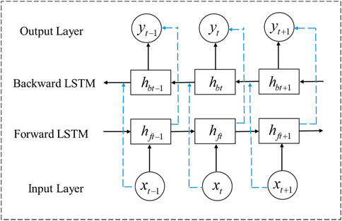
Figure 1. BiLSTM network structure (Wu, 2021).

The basic architecture of the BiLSTM model includes a forward LSTM and a backward LSTM, allowing it to simultaneously explore the temporal characteristics of both forward and backward data sequences. The forward computation process of the BiLSTM neural network is shown in Equation 11:

$h_{ft}=H\left(x_t,h_{ft-1}\right)(11)$

where x_t is input feature matrix and h_ft is the forward hidden state, and H represents the computation process of the LSTM network.

The backward computation process of the BiLSTM neural network is shown in Equation 12:

$h_{bt}=H\left(x_t,h_{bt-1}\right)(12)$

where h_bt is the backward hidden state, and H represents the computation process of the LSTM network.

The final output of the BiLSTM model is shown in Equation 13:

$h_t=w_{ft}{h}_{ft}+w_{bt}{h}_{bt}(13)$

where w_ft and w_bt are the weights of the forward and backward hidden layer outputs, respectively.

The LSTM network contains three logical units: the input gate, forget gate, and output gate, which control the output of the memory unit. The specific computation processes are as follows shown in Equations 14–19:

$i_t=\sigma \left(W_i\left(x_t,h_{t-1}\right)+b_i\right)(14)$

$f_t=\sigma \left(W_f\left(x_t,h_{t-1}\right)+b_f\right)(15)$

$o_t=\sigma \left(W_o\left(x_t,h_{t-1}\right)+b_o\right)(16)$

$C_t=\tanh \left(W_c\left(x_t,h_{t-1}\right)+b_c\right)(17)$

$c_t=i_t\cdot C_t+f_t\cdot c_{t-1}(18)$

$h_{ft/bt}=o_t\cdot \tanh \left(c_t\right)(19)$

where x_t is input feature matrix, σ and tanh are the activation functions. i, f, o present input, forget and output gate, respectively. W and b are the weights and biases of the respective gates, and c_t represents the state of the memory storage unit, which is the core of the LSTM.

Theoretically, this bidirectional capability allows BiLSTM to better model complex temporal dependencies, such as cyclical weather patterns and abrupt changes in power output. In wind and PV systems, future conditions (e.g., changes in sunlight intensity or wind speed) can influence the current output, just as past conditions do. BiLSTM’s structure makes it well-suited to learn from these bidirectional temporal dependencies, thereby improving prediction accuracy. While GRU offers computational efficiency, BiLSTM’s enhanced contextual understanding aligns better with the intricate dynamics of renewable energy output, making it a more robust choice for this application.

5.2 Overall Wind-PV prediction framework

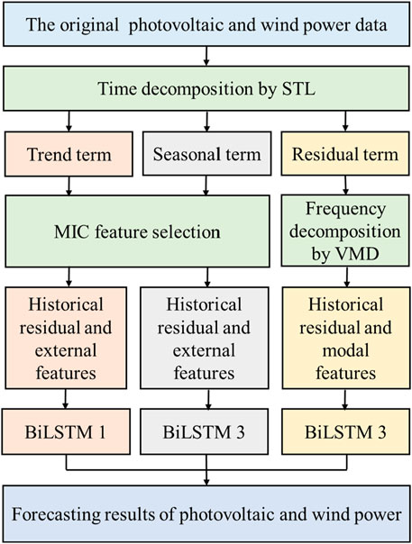
In summary, as shown in Figure 2, to achieve short-term power output forecasting for wind and PV power generation, this paper integrates time domain decomposition, frequency domain decomposition, the MIC, and the BiLSTM model into a unified prediction framework. First, the original wind and PV data are subjected to time domain decomposition to extract trend, seasonal, and residual components. Then, the residual component undergoes VMD to extract modal functions of different frequencies. Next, the MIC method is used to select features highly correlated with power output. Finally, the selected features are input into the BiLSTM model for training and prediction.

Figure 2

Figure 2. Overall Wind-PV prediction framework.

5.3 Prediction error evaluation metrics

To evaluate the performance of the prediction model, various typical prediction error evaluation metrics are used, including Root Mean Square Error (RMSE) and Mean Absolute Error (MAE) (Sanjari et al., 2019).

RMSE is shown in Equation 20:

$\text{RMSE}=\sqrt{\frac{1}{n}{\displaystyle \sum _{i=1}^n}{\left(y_i-{\widehat{y}}_i\right)}^2}(20)$

MAE is shown in Equation 21:

$\left.\text{MAE}=\frac{1}{n}\left.{\displaystyle \sum _{i=1}^n}\right|y_i-{\widehat{y}}_i\right|(21)$

where y_i is the actual value, ${\widehat{y}}_i$ is the predicted value, and n is the number of samples.

It is worth noting that the inclusion of these alternative metrics would not alter the feasibility or overall performance of the proposed method.

6 Case study

This paper utilizes actual historical data from a typical PV station and wind power station in Hebei Province, China for short-term wind and PV power output prediction. The data from the PV and wind stations in Hebei Province were selected because Hebei is known for its significant deployment of wind and solar energy systems, making it representative of typical renewable energy generation conditions in China. The data range from July to August 2023. In addition to wind and PV output data, meteorological data such as PV radiation, wind speed, and temporal data like weekdays and hours are used. Among them, the time resolution of the data is 15 min, week is displayed according to the date, from number 1 to 7, and hour is from number 1 to 24. First, the data are preprocessed by using quartile method to eliminating outlier and linear interpolation to fill in missing data. Then, the load, meteorological, and temporal data are normalized by the min-max normalization method as shown in Equation 22:

$x^{\prime }=\frac{x-x_{\min }}{x_{\max }-x_{\min }}(22)$

where x is the normalized feature data, ranging from 0 to 1, x is the original feature variable, and x_max and x_min are the maximum and minimum values of the feature variable, respectively.

6.1 Results of time domain decomposition based on STL

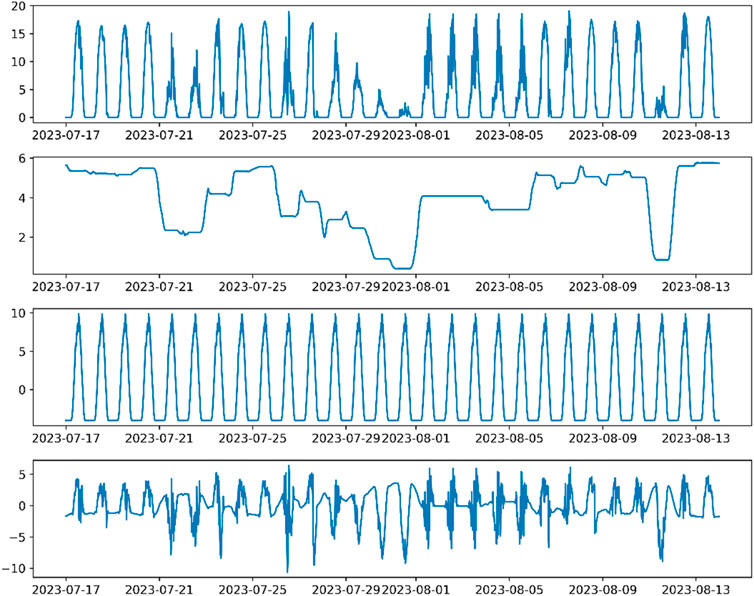
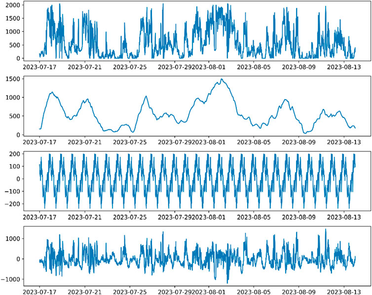
Fully utilizing the PV and wind power data, considering the inherent temporal characteristics of wind-PV output data, the STL method is employed to extract these features. Figures 3, 4 show the time domain decomposition results for PV and wind power output, respectively.

Figure 3

Figure 3. Time domain decomposition results for PV output.

Figure 4

Figure 4. Time domain decomposition results for wind power output.

From Figure 3, it can be seen that the trend component of PV output exhibits fluctuations. For instance, there is a downward trend on July 21 and July 22, followed by an upward trend. Between July 29 and July 31, the PV output shows a decreasing trend, then stabilizes. This reveals the trend patterns in PV output. The seasonal component shows periodic fluctuations with a small variation pattern, reflecting the baseline power of PV output. The residual component has strong volatility and randomness with highly uncertain waveform patterns. Figure 4 shows that the complex original wind power output is decomposed into a smoother trend component, a periodic seasonal component, and a random residual component. Therefore, STL decomposition can extract regular trend and seasonal components from complex original sequences, effectively enhancing the learning and training efficiency of wind-PV prediction models.

6.2 Results of frequency domain decomposition based on VMD

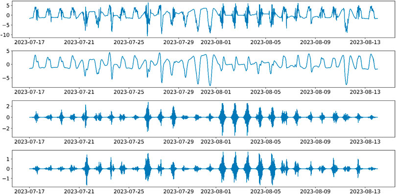
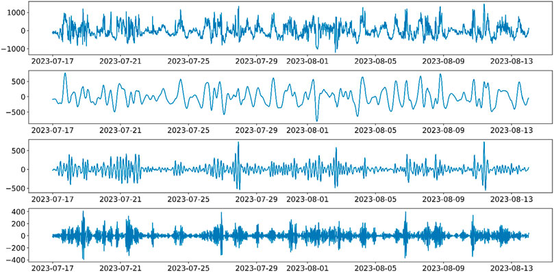
The residual component significantly influences wind-PV power output prediction. This paper uses VMD to perform frequency domain decomposition on the residual component, extracting its characteristic patterns and obtaining different modal forms of residual power, thus reducing the uncertainty of the residual component. Figures 5, 6 show the frequency domain decomposition results of PV and wind residual components, respectively, when the number of modal features is 3.

Figure 5

Figure 5. Frequency domain decomposition results for PV residual component.

Figure 6

Figure 6. Frequency domain decomposition results for wind residual component.

From the decomposed modes 1 to 3, it is evident that the frequency and volatility of the components increase progressively. Mode 1, with the highest proportion, represents the trend changes of the residual component. Modes 2 and 3 reflect the fluctuation patterns of the residual component at different frequencies. Therefore, modes 1 to 3 can be used as input features for the wind-PV prediction model, reflecting the uncertainty and inherent frequency domain patterns of the residual component to a certain extent, thereby fitting future residual fluctuations.

6.3 Prediction model input feature selection based on MIC

Based on the time-frequency decomposition of the original wind-PV data, time-frequency data reflecting the operational characteristics of wind-PV power were obtained. The features considered in this paper include internal features like historical wind-PV data and time-frequency data, as well as external features such as PV radiation, wind speed, weekdays, and hours. MIC is used to select features highly correlated with the original wind-PV and time-frequency data as input features for the prediction model.

The MIC analysis results, as shown in Figure 7, indicate that the correlation between the original PV data and weekdays is low, while the correlation between the original wind data and its historical internal features is low, with a weak correlation with temporal features. This suggests that the original wind-PV data contain complex and coupled features, making it difficult for MIC to directly analyze the accurate correlation between internal and external features. On the other hand, using the decoupled trend and seasonal components, which represent the temporal scale changes of the original wind-PV data, allows MIC to better explore the correlation between decomposition components and features. This paper selects internal and external features with MIC values greater than 0.3 as input features for the prediction model. For PV seasonal components, historical seasonal power, PV radiation, and hour are used as input features for the seasonal component prediction model. For wind seasonal components, historical seasonal power and hour are used as input features. For PV trend components, historical trend power, PV radiation, and weekdays are used as input features. For wind trend components, historical trend power, wind speed, and weekday are used as input features. The residual component’s certainty is high, so it does not undergo MIC correlation analysis. Instead, historical data of the residual component and modal features obtained from VMD frequency domain decomposition are used as input features for the residual component prediction model.

Figure 7

Figure 7. Feature Correlation Analysis Results based on MIC. (A) PV (B) Wind.

6.4 Time-frequency decomposition prediction experiment for Wind-PV power

To verify the effectiveness of the proposed wind-PV time-frequency decomposition prediction method, the following three prediction cases are set up for experimentation:

Case 1:. Using the BiLSTM model, input the features selected by MIC to directly predict the original wind-PV output data without decomposition.

Case 2:. Using the BiLSTM model, input the features selected by MIC to predict the seasonal, trend, and residual components of wind-PV data decomposed in the time domain.

Case 3:. Using the BiLSTM model, input the features selected by MIC to predict the seasonal and trend components of wind-PV data decomposed in the time domain. The residual component undergoes frequency domain decomposition using VMD, and the obtained modal features are used as input for the residual component prediction.

The BiLSTM model built in this paper uses the tanh activation function, with one hidden layer and a learning rate of 0.01. The hyperparameter settings of are determined by GridSearch method. The core principle is to cross validate each set of parameters by traversing parameter grid, and evaluate the performance of each set of parameters according to scoring metrics. Finally, the parameter combination that makes the score index optimal is selected as the final hyperparameter configuration. Cross-validation is performed using the grid method based on the parameter range in Table 1 to select the optimal hyperparameters for the prediction model.

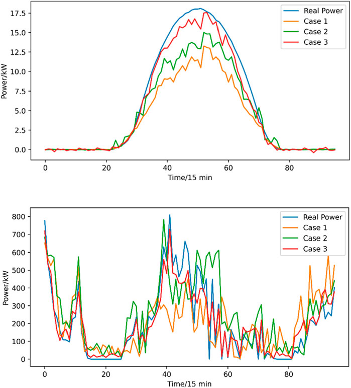
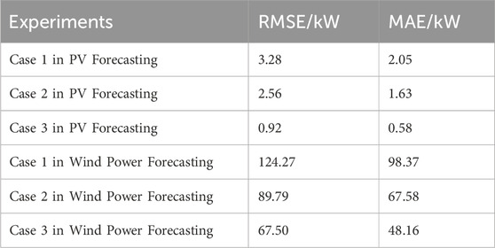
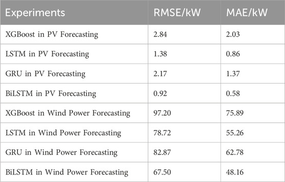
Figure 8 and Table 2 show the wind-PV prediction results for the different experimental cases mentioned above. From the figures, it can be seen that Case 3’s PV and wind power outputs best fit the original wind-PV output curves. The average RMSE and MAE values for PV and wind power predictions in Case 1 are 3.28 and 124.27, and 2.05 and 98.37, respectively. Due to the smaller power base of PV output, the prediction error is lower compared to wind power. Additionally, it can be seen from the table that Case 2’s wind-PV prediction error is lower than Case 1, indicating that decomposing wind-PV output data into three time-domain components allows the BiLSTM to better learn the temporal variation patterns of the load. Finally, it is evident that Case 3 achieves the minimum RMSE prediction errors of 0.92 for PV and 67.50 for wind power, with MAE values of 0.58 and 48.16. Compared to Case 2, this indicates that using only historical residual values as input features makes it difficult for the prediction model to directly learn the highly random residual component patterns. However, decomposing the residual component using VMD and using the extracted modal features as input for the residual component prediction model simplifies the complex residual fluctuations, improving the prediction accuracy of both the residual component and the overall wind-PV power output.

In conclusion, the time-frequency decomposition method effectively captures the fluctuation patterns in wind-PV time series, enhancing the accuracy of wind-PV power output prediction.

Table 1

Table 1. Hyperparameter range for BiLSTM prediction model.

Figure 8

Figure 8. Wind-PV power prediction results.

Table 2

Table 2. Prediction errors of Wind-PV models.

6.5 Comparison experiment with various prediction models

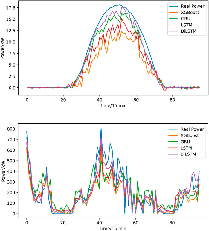
Based on time-frequency decomposition and MIC feature selection, Figure 9 and Table 3 show the wind-PV prediction results for different models. From the figures, it is clear that the proposed BiLSTM prediction model has a strong generalization ability for time series. Compared to LSTM, the RMSE and MAE errors of PV output through the proposed BiLSTM decreased by an average of 0.46 and 0.28, respectively, while the RMSE and MAE errors of wind power output through the proposed BiLSTM decreased by 11.22 and 7.04, respectively. GRU, being a simplified version of the gated state, is simpler compared to LSTM, thus limiting the fitting effect of the wind-PV prediction model. In addition, XGBoost has limited ability to mine the time-series data of wind and PV power, so the prediction error RMSE and MAE is the largest in PV with 2.84 and 2.03. Besides, the prediction error RMSE and MAE is the largest in wind power by XGBoost with 97.20 and 75.89. In summary, the BiLSTM prediction model framework proposed in this paper comprehensively considers the variations of wind-PV sequences in both time and frequency domains, deeply exploring the implicit long-term and short-term dependencies in the wind-PV time series, thereby exhibiting superior prediction performance.

Figure 9

Figure 9. Wind-PV power prediction results.

Table 3

Table 3. Prediction errors of Wind-PV models.

7 Conclusion

The proposed wind and PV power output forecasting framework based on time-frequency decomposition and BiLSTM effectively improves the accuracy of wind and PV power generation forecasting by combining time domain and frequency domain decomposition techniques. The attention mechanism in BiLSTM and probability prediction of PV and wind power can be carried out in the future research work. The specific conclusions are as follows:

1) By extracting trend and seasonal components using the STL method and applying VMD to decompose the residual component in the frequency domain, regular features can be extracted from complex original data, enhancing the learning efficiency and accuracy of the prediction model.

2) The MIC method effectively selects features highly correlated with wind and PV power output, improving model performance. The results indicate that selecting appropriate input features is crucial for enhancing the prediction accuracy of the model.

3) Compared to traditional LSTM and GRU, the BiLSTM demonstrates higher accuracy and reliability in handling time series forecasting tasks for wind and PV power generation. This is relying on the BiLSTM ability of consider both past and future relationships in the time series, capturing temporal features more accurate.

Several other enhancements could be explored in future research. These include integrating ensemble learning techniques to combine the strengths of multiple models, applying multivariate forecasting to jointly predict power generation from various sources, and utilizing data augmentation methods, such as GANs, to improve model generalization with limited data. Additionally, enhancing model interpretability through explainable AI techniques like SHAP or lime could provide more transparency in decision-making.

Data availability statement

The original contributions presented in the study are included in the article/supplementary material, further inquiries can be directed to the corresponding author.

Author contributions

YZ: Conceptualization, Methodology, Software, Writing–original draft. XF: Conceptualization, Software, Writing–review and editing. YW: Formal Analysis, Software, Visualization, Writing–review and editing. ZW: Investigation, Validation, Writing–review and editing. XW: Data curation, Investigation, Writing–review and editing.

Funding

The author(s) declare financial support was received for the research, authorship, and/or publication of this article. This research was funded by the North China Electric Power Research Institution Co., Ltd. (Project Name: Research on technology for improving short-term power forecasting of new energy based on multi-source data fusion, grant number: KJZ2023024).

Conflict of interest

Authors YZ, XF, YW, ZW, and XW were employed by North China Electric Power Research Institution Co., Ltd.

The authors declare that this study received funding from the North China Electric Power Research Institution Co., Ltd. The funder had the following involvement in the study: Study design and collection.

Publisher’s note

All claims expressed in this article are solely those of the authors and do not necessarily represent those of their affiliated organizations, or those of the publisher, the editors and the reviewers. Any product that may be evaluated in this article, or claim that may be made by its manufacturer, is not guaranteed or endorsed by the publisher.

References

An, G., Jiang, Z., Cao, X., Liang, Y., Zhao, Y., Li, Z., et al. (2021). Short-term wind power prediction based on particle swarm optimization-extreme learning machine model combined with AdaBoost algorithm. IEEE access 9, 94040–94052. doi:10.1109/access.2021.3093646

CrossRef Full Text | Google Scholar

Azam, M. F., and Younis, M. S. (2021). Multi-horizon electricity load and price forecasting using an interpretable multi-head self-attention and EEMD-based framework. IEEE Access 9, 85918–85932. doi:10.1109/access.2021.3086039

CrossRef Full Text | Google Scholar

Bacanin, N., Jovanovic, L., Zivkovic, M., Kandasamy, V., Antonijevic, M., Deveci, M., et al. (2023). Multivariate energy forecasting via metaheuristic tuned long-short term memory and gated recurrent unit neural networks. Inf. Sci. 642, 119122. doi:10.1016/j.ins.2023.119122

CrossRef Full Text | Google Scholar

Chen, D., Zhang, J., and Jiang, S. (2020). Forecasting the short-term metro ridership with seasonal and trend decomposition using loess and LSTM neural networks. IEEE Access 8, 91181–91187. doi:10.1109/access.2020.2995044

CrossRef Full Text | Google Scholar

Dey, R., and Salem, F. M. (2017). “Gate-variants of gated recurrent unit (GRU) neural networks,” in 2017 IEEE 60th international midwest symposium on circuits and systems (MWSCAS), Boston, USA, 06-09 August 2017 (IEEE), 1597–1600.

CrossRef Full Text | Google Scholar

Dong, Y., Yang, T., Xing, Y., Du, J., and Meng, Q. (2023). Data-driven modeling methods and techniques for pharmaceutical processes. Processes 11 (7), 2096. doi:10.3390/pr11072096

CrossRef Full Text | Google Scholar

Dragomiretskiy, K., and Zosso, D. (2014). Variational mode decomposition. IEEE Trans. Signal Process. 62 (3), 531–544. doi:10.1109/tsp.2013.2288675

CrossRef Full Text | Google Scholar

El-Kenawy, E. S. M., Mirjalili, S., Khodadadi, N., Abdelhamid, A. A., Eid, M. M., El-Said, M., et al. (2023). Feature selection in wind speed forecasting systems based on meta-heuristic optimization. Plos one 18 (2), e0278491. doi:10.1371/journal.pone.0278491

PubMed Abstract | CrossRef Full Text | Google Scholar

Fu, Y., Chai, H., Zhen, Z., Wang, F., Xu, X., Li, K., et al. (2021). Sky image prediction model based on convolutional auto-encoder for minutely solar PV power forecasting. IEEE Trans. Industry Appl. 57 (4), 3272–3281. doi:10.1109/tia.2021.3072025

CrossRef Full Text | Google Scholar

Harrou, F., Sun, Y., Taghezouit, B., Dairi, A., and Khadraoui, S. (2024). Editorial: advanced data-driven methods for monitoring solar and wind energy systems, volume II. Front. Energy Res. 12, 1365496. doi:10.3389/fenrg.2024.1365496

CrossRef Full Text | Google Scholar

Jiang, B., Liu, Y., Geng, H., Wang, Y., Zeng, H., and Ding, J. (2022). A holistic feature selection method for enhanced short-term load forecasting of power system. IEEE Trans. Instrum. Meas. 72, 1–11. doi:10.1109/tim.2022.3219499

CrossRef Full Text | Google Scholar

Joshi, R., Ghosh, J., Kalani, N., and Tanna, R. L. (2024). Assessment of stacked LSTM, bidirectional LSTM, ConvLSTM2D, and auto encoders LSTM time series regression analysis at ADITYA-U tokamak. IEEE Trans. Plasma Sci. 52, 2403–2409. doi:10.1109/tps.2024.3355283

CrossRef Full Text | Google Scholar

Li, Z., Xu, Y., Wang, P., and Xiao, G. (2023). Restoration of a multi-energy distribution system with joint district network reconfiguration via distributed stochastic programming. IEEE Trans. Smart Grid 15, 2667–2680. doi:10.1109/tsg.2023.3317780

CrossRef Full Text | Google Scholar

Lyu, C., Eftekharnejad, S., Basumallik, S., and Xu, C. (2022). Dynamic feature selection for solar irradiance forecasting based on deep reinforcement learning. IEEE Trans. Industry Appl. 59 (1), 533–543. doi:10.1109/tia.2022.3206731

CrossRef Full Text | Google Scholar

Mayer, M. J., and Yang, D. (2023). Pairing ensemble numerical weather prediction with ensemble physical model chain for probabilistic photovoltaic power forecasting. Renew. Sustain. Energy Rev. 175, 113171. doi:10.1016/j.rser.2023.113171

CrossRef Full Text | Google Scholar

Mo, J., Wang, R., Cao, M., Yang, K., Yang, X., and Zhang, T. (2022). A hybrid temporal convolutional network and Prophet model for power load forecasting. Complex and Intelligent Syst. 9, 4249–4261. doi:10.1007/s40747-022-00952-x

CrossRef Full Text | Google Scholar

Pavlov-Kagadejev, M., Jovanovic, L., Bacanin, N., Deveci, M., Zivkovic, M., Tuba, M., et al. (2024). Optimizing long-short-term memory models via metaheuristics for decomposition aided wind energy generation forecasting. Artif. Intell. Rev. 57 (3), 45. doi:10.1007/s10462-023-10678-y

CrossRef Full Text | Google Scholar

Sanjari, M. J., Gooi, H. B., and Nair, N. K. C. (2019). Power generation forecast of hybrid PV–wind system. IEEE Trans. Sustain. Energy 11 (2), 703–712. doi:10.1109/tste.2019.2903900

CrossRef Full Text | Google Scholar

Sankarananth, S., Karthiga, M., Suganya, E., S., S., and Bavirisetti, D. P. (2023). AI-enabled metaheuristic optimization for predictive management of renewable energy production in smart grids. Energy Rep. 10, 1299–1312. doi:10.1016/j.egyr.2023.08.005

CrossRef Full Text | Google Scholar

Stoean, C., Zivkovic, M., Bozovic, A., Bacanin, N., Strulak-Wójcikiewicz, R., Antonijevic, M., et al. (2023). Metaheuristic-based hyperparameter tuning for recurrent deep learning: application to the prediction of solar energy generation. Axioms 12 (3), 266. doi:10.3390/axioms12030266

CrossRef Full Text | Google Scholar

Strielkowski, W., Vlasov, A., Selivanov, K., Muraviev, K., and Shakhnov, V. (2023). Prospects and challenges of the machine learning and data-driven methods for the predictive analysis of power systems: a review. Energies 16 (10), 4025. doi:10.3390/en16104025

CrossRef Full Text | Google Scholar

Su, Y., Teh, J., and Chen, C. (2023). Optimal dispatching for AC/DC hybrid distribution systems with electric vehicles: application of cloud-edge-device cooperation. IEEE Trans. Intelligent Transp. Syst. 25, 3128–3139. doi:10.1109/tits.2023.3314571

CrossRef Full Text | Google Scholar

Tan, M., Hu, C., Chen, J., Wang, L., and Li, Z. (2022). Multi-node load forecasting based on multi-task learning with modal feature extraction. Eng. Appl. Artif. Intell. 112, 104856. doi:10.1016/j.engappai.2022.104856

CrossRef Full Text | Google Scholar

Walczewski, M. J., and Wöhrle, H. (2024). Prediction of electricity generation using onshore wind and solar energy in Germany. Energies 17 (4), 844. doi:10.3390/en17040844

CrossRef Full Text | Google Scholar

Wang, S., Deng, X., Chen, H., Shi, Q., and Xu, D. (2021). A bottom-up short-term residential load forecasting approach based on appliance characteristic analysis and multi-task learning. Electr. Power Syst. Res. 196, 107233. doi:10.1016/j.epsr.2021.107233

CrossRef Full Text | Google Scholar

Wen, T., Dong, D., Chen, Q., Chen, L., and Roberts, C. (2019). Maximal information coefficient-based two-stage feature selection method for railway condition monitoring. IEEE Trans. Intelligent Transp. Syst. 20 (7), 2681–2690. doi:10.1109/tits.2018.2881284

CrossRef Full Text | Google Scholar

Wu, Z. (2021). “The comparison of forecasting analysis based on the ARIMA-LSTM hybrid models,” in 2021 International Conference on E-Commerce and E-Management (ICECEM), Dalian, China, 24-26 September 2021 (IEEE), 185–188.

CrossRef Full Text | Google Scholar

Xuan, Y., Si, W., Zhu, J., Sun, Z., Zhao, J., Xu, M., et al. (2021). Multi-model fusion short-term load forecasting based on random forest feature selection and hybrid neural network. Ieee Access 9, 69002–69009. doi:10.1109/access.2021.3051337

CrossRef Full Text | Google Scholar

Yan, J., Hu, L., Zhen, Z., Wang, F., Qiu, G., Li, Y., et al. (2021). Frequency-domain decomposition and deep learning based solar PV power ultra-short-term forecasting model. IEEE Trans. Industry Appl. 57 (4), 3282–3295. doi:10.1109/tia.2021.3073652

CrossRef Full Text | Google Scholar

Yang, M., Ju, C., Huang, Y., Guo, Y., and Jia, M. (2024). Short-term power forecasting of wind farm cluster based on global information adaptive perceptual graph convolution network. IEEE Trans. Sustain. Energy 15, 2063–2076. doi:10.1109/tste.2024.3397877

CrossRef Full Text | Google Scholar

Zhang, C., Fu, Y., and Gong, L. (2022a). Short-term electricity price forecast using frequency analysis and price spikes oversampling. IEEE Trans. Power Syst. 38 (5), 4739–4751. doi:10.1109/tpwrs.2022.3218712

CrossRef Full Text | Google Scholar

Zhang, R., Chen, Y., Li, Z., Jiang, T., and Li, X. (2024). Two-stage robust operation of electricity-gas-heat integrated multi-energy microgrids considering heterogeneous uncertainties. Appl. Energy 371, 123690. doi:10.1016/j.apenergy.2024.123690

CrossRef Full Text | Google Scholar

Zhang, X., Kuenzel, S., Colombo, N., and Watkins, C. (2022b). Hybrid short-term load forecasting method based on empirical wavelet transform and bidirectional long short-term memory neural networks. J. Mod. Power Syst. Clean Energy 10 (5), 1216–1228. doi:10.35833/mpce.2021.000276

CrossRef Full Text | Google Scholar

Zhong, J., Li, Y., Wu, Y., Cao, Y., Li, Z., Peng, Y., et al. (2023). Optimal operation of energy hub: an integrated model combined distributionally robust optimization method with stackelberg game. IEEE Trans. Sustain. Energy 14 (3), 1835–1848. doi:10.1109/tste.2023.3252519

CrossRef Full Text | Google Scholar