- 1Power Dispatch Center of State Grid Gansu Electric Power Company, Lanzhou, China
- 2Department of Electrical Engineering and Information Engineering, Lanzhou University of Technology, Lanzhou, China
- 3Electric Power Science Research Institute of State Grid Gansu Electric Power Company, Lanzhou, China
- 4School of Electronics and Information Engineering Southwest Petroleum University, Chengdu, China
- 5School of Electrical Engineering, Northwest University for Nationalities, Lanzhou, China
The short-term fluctuation of wind power can affect its prediction accuracy. Thus, a short-term segmentation prediction method of wind power based on ramp segment division is proposed. A time-series trend extraction method based on moving average iteration is proposed on the full-time period to analyze the real-time change characteristics of power time-series initially; secondly, a ramp segment extraction method based on its definition and identification technique is proposed based on the results of the trend extraction; and a segmentation prediction scheme is proposed to lean the power prediction under different time-series: the LightGBM-LSTM is proposed for the non-ramping segment using point prediction, and the CNN-BiGRU-KDE is proposed for probabilistic prediction of ramp segments. From the results, this ramp segment definition and identification technique can effectively identify the ramp process of wind power, which makes up for the misidentification and omission of the classical climbing event definition; meanwhile, the segment prediction scheme not only meets the prediction accuracy requirements of the non-ramping segment, but also provides the effective robust information for the prediction of the ramping period, which offers reliable reference information for the actual wind farms. In particular, it is well adapted to wind power prediction under extreme working conditions caused by ramping weather, which is a useful addition to short-term wind power prediction research.
1 Introduction
In 2020, with the deepening understanding of the “dual-carbon” goal by all parties in society, China has put forward the goal of “2030 carbon peak, 2060 carbon neutral” (State Grid, 2021), and wind power is ushering in rapid development. Wind power is difficult to predict due to its unique stochasticity and instability, which poses a great challenge to the reliable operation of wind farms and smart energy systems. With the development of China’s power marketization, accurate and efficient short-term wind power prediction is especially important to enhance the capacity of wind power consumption and promote the efficient interaction of source, grid, and load (Lefeng et al., 2022; Lefeng et al., 2021; Lefeng et al., 2020). Currently, there is a lack of in-depth research on the short-term power prediction method for wind power over the whole period considering the weather in the climbing segment (Cheng and Yu, 2019).
Existing short-term power prediction methods for wind power can be divided into two kinds: the physical method (Ernst et al., 2007) and the data-driven method (Wang et al., 2022). Among them, the former is built based on the atmospheric motion portrayal, according to the meteorological environment, geographic factors, and other information, the use of hydrodynamics and other physical laws to establish a model, focusing on the optimization of the boundary conditions and physical solution rules, with the characteristics of modeling difficulties, large computational volume, and therefore poor timeliness, is generally suitable for medium- and long-term forecasting (Cassola and Burlando, 2012). The latter takes the establishment of linear or nonlinear mapping between relevant meteorological features and power time series as the main means, emphasizes the search for intrinsic laws from multi-source, multi-dimensional, and multi-modal data, and has been widely used because of its better prediction accuracy (Zhou et al., 2021).
Existing studies usually categorize data-driven methods into deterministic forecasting and uncertainty forecasting based on the result presentation. Among them, the existing deterministic wind power prediction methods mainly include Auto-regressive and moving average (ARMA) (Erdem and Shi, 2011), Convolutional Neural Networks (CNN) (Men et al., 2016), and vector machines (Hu et al., 2014). Deterministic methods can form a mathematical abstract mapping relationship between inputs and outputs through data mining and machine learning and are suitable for power time series with gentle curve fluctuations. Specifically, literature (Meng et al., 2021) proposes a parameter optimization-based attention mechanism for accelerating the early prediction model to mine the temporal correlation of the input series-gated recurrent unit (GRU) short-term wind power prediction model; literature (Zhou et al., 2021) proposes a wind power prediction model that introduces the volatility hierarchical error correction model, which is based on the improvement of long-term recurrent convolutional neural network. All of the above literature has improved the prediction accuracy to a certain extent, and better prediction results can be achieved under normal fluctuating power hours. However, in the face of the ramping section of the weather under the fluctuating power, a single use of the above deterministic prediction methods will not be able to quantify the prediction error, and the stability of the prediction results is poor, and the combination of prediction techniques is applied and born (Gao et al., 2016; Liu et al., 2024). At the same time, due to the more complex and variable wind power scenarios, it poses a more serious challenge to the prediction methods. For this reason, we have carried out an in-depth study of the problems and difficulties existing in the current wind power prediction work.
Uncertainty prediction is a probabilistic interval prediction method represented by kernel density estimation (KDE) (Wang et al., 2024; Haoyi et al., 2023). Uncertainty prediction considers the randomness of the results, quantifies the prediction error, provides more information compared to the traditional point estimation, and can significantly improve the effectiveness of power hour prediction under weather in the climbing section (Jianhou et al., 2024). Specifically, literature (Wang et al., 2024) introduces a new offshore wind speed point and interval prediction model that combines an innovative two-layer decomposition technique, GRU and KDE. However, the lack of a typical power scenario delineation leads to a low prediction accuracy of the model for some power periods. Literature (Zareipour et al., 2011a; Cui et al., 2019) proposes data-driven probabilistic wind power ramp prediction methods based on massive simulated scenarios, but such models have yet to improve their robustness under weather in the ramp section. Literature (Ouyang et al., 2019) proposes an integrated learning method to generate probabilistic prediction results, but the method does not take into account the interference of power timing pseudo-inflection points on the complete extraction of the ramp segment period and does not highlight the improvement of the model’s accuracy under ramp segment weather. The above uncertainty prediction method improves the performance of wind power prediction under complex meteorological conditions to a certain extent, but there are still the following shortcomings: first, the lack of targeted optimization of the ramp segment of the extreme weather caused by the sudden change of power scenarios, which affects the prediction accuracy; second, the deterministic prediction method of the gentle power period is sufficient to meet the demand for prediction accuracy and stability, and the uncertain prediction takes up a large number of computing resources and the prediction interval under the gentle power period is too long to meet the prediction accuracy and stability requirements. Second, the deterministic prediction method is sufficient to meet the demand for prediction accuracy and stability in the gentle power period, while the uncertainty prediction takes up a lot of computing resources and the prediction interval is too large in the gentle power period, which affects the reasonableness and intuition of prediction.
The basis of ramp prediction is its identification technology. There have been in-depth studies on the research of wind power ramp events abroad, but the definition of it by various research institutions has not yet formed a unified standard. Literature (Potter et al., 2009; Ferreira et al., 2011) summarized four different definitions of ramp events by considering several factors such as power amplitude change, duration, and ramping rate. According to Truewind (2008), the occurrence of a “ramp event” is accompanied by a large change in wind speed in a short period, and the larger the amplitude change, the smaller the duration, and the faster the ramping rate, the more serious the ramp event is. Common studies set the minimum threshold of climb duration at 1 h, but ramp events of less than 1 h are also possible (Kamath, 2010; Kamath, 2011). Further, the literature (Zheng and Kusiak, 2009; Zareipour et al., 2011b) used a mean clustering algorithm and support vector machine to classify the ramp events in the historical data, respectively, and analyzed the characteristics and hazards of different types of ramp events.
The recognition technology of ramp events in China is not mature, and it is based on power prediction. Literature (Greaves et al., 2009) used a numerical weather prediction system to identify possible future wind power’s ramp events by obtaining meteorological background information. In literature (Cui et al., 2014; Huang et al., 2016; Ouyang et al., 2017), ARMA, Kalman, and neural network models were used to predict the power first, and then the predicted power was used for ramp recognition. Due to the lack of consideration of the characteristics of ramp events, the effectiveness of these methods in the identification of ramp events is very limited, which makes the identification of ramp events one of the urgent problems to be solved in the grid connection of wind power.
Aiming at the above deficiencies, a short-term wind power segmentation prediction method based on ramp period division is proposed in this paper. Specifically, a trend extraction model based on the moving average sensitivity method (MASM) is first proposed for the whole period to characterize the real-time change of power time series preliminarily; furthermore, a hill-ramp segment definition and identification method is proposed to extract the hill-ramp power period for the sub-time period; finally, a segmented prediction method is proposed to make lean prediction of wind power for the whole period: a light gradient boosting machine (LightGBM) - Long short-term memory (LSTM) is proposed for the non-hill-ramp segment period. Finally, a segmented prediction method is proposed to make a lean prediction of wind power for the whole period: a LightGBM-LSTM combination prediction method is proposed for the non-ramp period; a probabilistic prediction method based on CNN-BiGRU-KDE is proposed for the ramp period. The experimental results show that the prediction accuracy of the method proposed in this paper is greatly improved compared with the existing methods, providing new ideas for short-term wind power prediction.
2 Basic idea
Changes in meteorological parameters under ramp segment weather are characterized by instantaneous sudden changes and drastic amplitude, which leads to many problems in wind power prediction under ramp segment weather conditions.
The main problems are as follows:
(1) As the weather in the ramp segment has various changes in meteorological patterns in a short period, it is easy to cause misjudgment of the trend, which affects the accuracy of power extraction in the ramp segment.
(2) Due to the strong stochasticity and complexity of the weather mutation period in the ramp segment, it is difficult to accurately and completely extract the power mutation period in the ramp segment by the power mutation period extraction method with the fixed characteristics as the extraction factor.
(3) Different meteorological models correspond to different time series characteristics in the ramp weather period. To fully utilize the performance advantages of deterministic and uncertainty prediction methods, it is one of the urgent problems to propose a segmented prediction strategy to match different weather patterns.
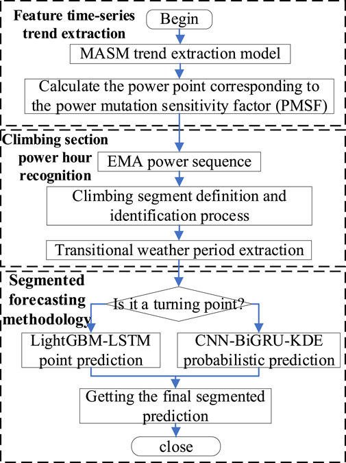
To address the above issues specifically, this paper proposes a segmented prediction method based on ramp segment identification and recognition technology. The specific method flow is shown in Figure 1. Firstly, the MASM model is used to extract the trend components in the time series, smoothing transitions and capturing trend changes. Subsequently, the power mutation sensitivity factor (PMSF) is employed to calculate specific power points of sudden changes, identify key changes in the time series, and obtain the exponential moving average (EMA) sequence. On this basis, ramp segments in EMA are identified and extracted by defining ramp segments and setting ramp thresholds (ramp amplitude, ramp rate), i.e., periods of significant changes in weather conditions, to analyze their impact on electricity demand. In the prediction phase, a segmented prediction method is adopted, processing the time series according to different characteristics or patterns.
For non-ramp segments, the LightGBM-LSTM model is used for point prediction, combining the advantages of gradient boosting and long short-term memory networks to capture complex patterns and temporal dependencies. For ramp segments, the CNN-BiGRU-KDE model is employed for probabilistic prediction, generating predictive probability distributions. Finally, the results of point prediction and probabilistic prediction are integrated to form the final segmented prediction. This method not only considers the accuracy of prediction but also incorporates prediction uncertainty, providing more comprehensive and reliable prediction results.
3 Time-series trend extraction
Under the weather of the ramp segment, the wind power shows drastic changes, to accurately identify the ramp power period, the first step is to extract the time series trend of the whole period. The traditional method of recognizing the time series mutation is to extract the index parameters such as mutation amplitude and mutation duration as the basis of identification. This method is only applicable to a single time-sequence mutation scenario, and it is easy to cause insufficient extraction of the mutation period for the complex and variable time-sequence mutation scenarios of the ramp segment. To establish an ideal early warning mechanism for weather periods in the ramp segment, this paper proposes a novel method of describing the time-sequence trend by taking the historical time-sequence characteristics into full consideration. Different from the traditional trend extraction method that directly takes the original time series as the feature extraction object, this method takes the moving average as the trend research object. It not only avoids the trend misjudgment caused by the raw power time series noise but also retains the timeliness of the time series change trend. This method extracts the time-series trend from the power curve 1 h before the point in time to be predicted.
MASM is a technical indicator that utilizes the aggregation and separation conditions between short-term averages and raw data combined with the time series characteristics of the averages themselves to investigate and judge the highs and lows of the prediction object (Li, 2013). The principle of MASM is to use the EMA that characterizes the short-term trend of the raw data and to compute the PMSF of the current instantaneous rate of change of the EMA. The PMSF can better project the inflection point of the trend after the comprehensive evaluation of the mutation sensitivity. The specific steps of MASM are as follows:
Find the N-day smoothed moving average X of t if
Where: t is the current time point; X is the N-day smoothed moving average of the time series at moment t;
The EMA curve obtained above is smoothed by the Gaussian window method, and the rate of change of each moment in the time sequence is further calculated as PMSF. The specific calculation is as follows:
Where:
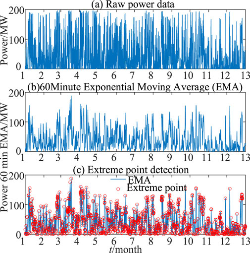
Figure 2. Schematic diagram of the effect of EMA and PMSF. (A) Raw power data. (B) 60 min Expontial Movieng Average (EMA). (C) Extreme Point detection.
4 Ramp segment identification
Considering that a ramp event is a large change in wind power over a short period, the wind power ramp event can be redefined by the ramp amplitude and ramp rate. In this paper, we will first find the extreme points of historical wind power sequences, and analyze and identify the ramp events based on the sequence of extreme points to avoid the identification of ramps under different definition criteria.
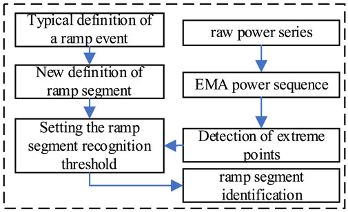
The current wind power ramp is generally studied as an “event”, and the complete ramp event consists of multiple ramp segments, so this paper will take the “ramp segment” as an object to study, and put forward a new approach to identify the ramp segment, the basic idea is shown in Figure 3.
As can be seen in Figure 3, on the one hand, the original wind power sequence is extracted from the extreme point to find out the extreme sequence; on the other hand, the new definition is determined by the typical definition of ramp events; the magnitude threshold and rate threshold are set in combination with the above two aspects to identify the ramp segment; finally, the feature analysis is carried out to determine the ramp segments in a specific region.
4.1 Extreme extraction process
The extreme extraction method achieves the effect of feature extraction by extracting the extreme values of the original sequence, by searching the local extreme points of the numerical sequence. Assuming that the original information matrix is X, X can be expressed as.
Where: X is the original data matrix;
1) Initialize the beginning and end of E as the beginning and end of X:
Where: E is the extreme matrix; d is the number of extreme points.
2) Give the discriminant of the extreme point:
If condition ① is met, it is a point of minimal value; if ② is met, it is a point of maximum value. Store
3) Correction for the beginning of the polar matrix.
Where:
(4) Extreme matrix terminal correction.
Where:
The above content provides a detailed introduction to the basic principles of the extreme extraction method and practical operation steps. We utilize the wind power data measured at a wind farm to verify the reliability of the extreme extraction method every 15 min, and the verification results are shown in Figure 2C.
The solid line in Figure 2C is the characteristic line of the extracted extreme points. From Figure 2C, it can be seen that the extreme extraction method can effectively extract the extreme points in the power series, and less extreme data can be used in the presentation of the change characteristics of the original series, to achieve the effect of data compression and achieve the purpose of feature extraction.
To facilitate the analysis of the following article, the extreme points are called temporary ramp points (TRP), and the E is called TRP series Y, that is:
Where: Y is the TRP matrix;
4.2 Definition of the ramp segment and threshold setting
4.2.1 Definition of a ramp segment
1) The classical definition of a ramp event.
Literature (Zhang et al., 2018; Freedman et al., 2008; Cutler et al., 2011) summarizes several typical definitions of ramp events.
Definition I. The condition is met if the difference between the power at the cutoff time and the power at the start time exceeds a set threshold λ within a given period [t, t+∆t].
Then the power ramp event is considered to occur in this time frame, where λ is the threshold of the ramp amplitude.
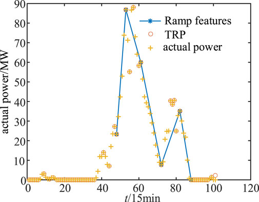
The literature (Zhang et al., 2018) recommends that a change in amplitude greater than about 15%–20% of the total installed capacity is recognized as a ramp event. The threshold of ramp magnitude for wind farms is used for the test, which results in an average value of about 30–40 MW. Figure 4 shows the ramp identification plot according to Definition I (Equation 11), taking λ = 35 MW.
From Figure 4, this definition recognizes simple ramp events in the power sequence. However, only the ramp amplitude is considered, and the ramp rate (the change characteristics of the power in the ramp process) is not considered, resulting in the loss of power characteristics. In addition, the ramp amplitude threshold set only based on the installed wind farm cannot effectively reflect the actual power amplitude change of the wind farm, which is easy to causes the omission of identification.
Definition II. Firstly, a time range [t, t+∆t] is circled, and then the maximum and minimum values are searched in this time range to find their extreme difference which is larger than λ, that is
Then the power ramp event is considered to occur in this time interval. Definition II considers the power amplitude in the time interval, while the rate of change is not characterized.
Definition III. Circle a certain time range [t, t+∆t], and when the power rate is greater than the value of β, it is the ramp rate in that time range:
Then the power ramp event is considered to occur within this time frame, where the β is the threshold for ramp rate. This definition is simultaneously able to determine the up-ramping and down-ramping situations. Equation 13 defines an up-ramp event when
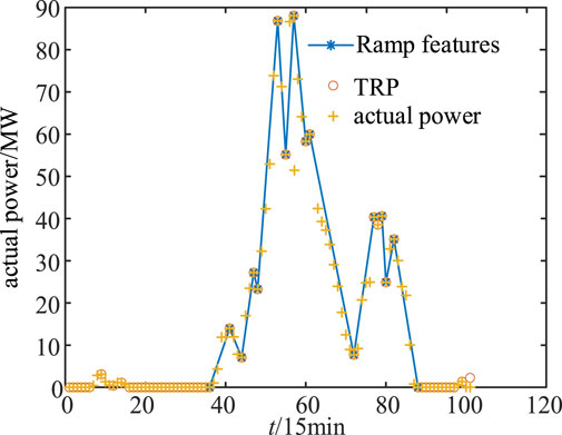
According to the literature (Truewind, 2008; Cutler et al., 2011), only when the power change of the wind farm reaches at least 50% of the installed capacity within 4 h is recognized as a ramp event, so the corresponding rate threshold can be calculated according to 0.417 MW/min. Combined with Equation 13, the ramp diagram identified by Definition III is drawn, as shown in Figure 5.
As can be seen in Figure 5, although the dynamics can be accurately depicted based on the ramp rate, the information redundancy of the ramp events is also increased by the extraction points with small change amplitude, leading to an unclear identification of the ramp events.
The definition of the above ramp event method identifies different results, which is not popularized in practical applications. And for the ramp events with complex processes and long periods, they are often interspersed with non-ramp intervals which cause ramp misrecognition. In the following segment, we will take a segmented approach, and based on the definition of a typical ramp event, we will define the ramp segment, and discuss and find the method of setting the ramp threshold.
2) A new type of ramp segment definition.
As can be seen from Figures 4, 5, it is difficult to recognize the complex process of ramp events by using Definitions I–III alone. In this paper, the ramp event is segmented, and Definitions I–III are combined and refined to redefine the ramp segment by combining (Equations 3–9) with the Y, as follows:
where
Equation 14 makes a limitation on the ramp amplitude (C1) and ramp rate (C2); when the C1 is available, the power rate between TRPs (Equation 10) is examined; when the C1 and C2 are satisfied at the same time, it is determined that the ramping has occurred between the TRPs, and the
Where: Z is the ramp point matrix;
The combination of condition I and condition II (Equation 12) makes the information redundancy better in complex ramp segments. Since
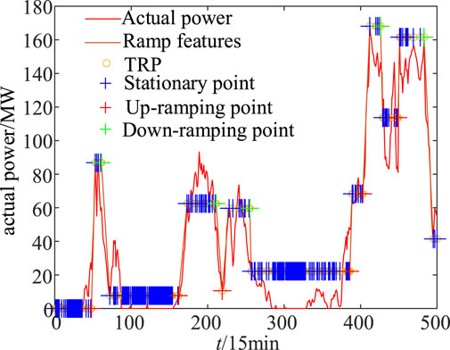
Equation 14 introduces the concept of stationary point (SP), defines the TRP with ramp amplitude less than λ or ramp rate less than β as a stationary point, and replaces the successive stationary points with a horizontal line, whose value is equal to the value of the starting stationary point. By introducing the concept of stationary point, clear statistics of the ramp period, reducing the redundancy of information in the ramp segment, and reducing the statistical error of ramp duration, we can effectively distinguish and recognize the calm and slow zones during power ramp.
4.2.2 Discussion of ramp threshold setting
1) Setting of β
C2 of Equation (14) already specifies the method for calculating the ramp rate. As shown in Figure 6A, the ramp rates of adjacent TRP are calculated and counted, and the confidence intervals of the ramp rates are analyzed by their cumulative probability distribution plots. Figure 6A shows that more than 90% of the ramp rates are less than βmax, indicating that the majority of the ramp rates can meet the grid connection
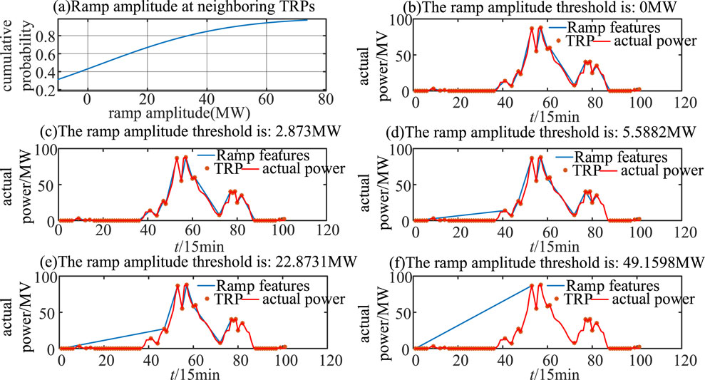
Figure 6. Ramp diagram under different ramp thresholds. (A) Ramp amplitude at neighboring TRPs. (B) The ramp amplitude threshold is 0 MW. (C) The ramp amplitude threshold is: 2.873 MW. (D) The ramp amplitude threshold is: 5.5882 MW. (E) The ramp amplitude threshold is: 22.8731 MW. (F) The ramp amplitude threshold is: 49.1598 MW.
Requirements, and more than 80% of the rates are greater than 0.417 MW/min. The ramp rate threshold for this wind farm is 0.4 MW/min, which can be obtained according to the recommendation of Literature (Huang et al., 2016), which indirectly verifies the validity of determining the ramp threshold by the method of mathematical statistics. According to the definition of Equation 14, when the rate of change of power in a certain time range is greater than a certain threshold value, it can be determined that the ramp may occur in this period. According to the mathematical and statistical results in Figure 6A, more than 80% of the power changes are contained in cases where the absolute value of the power rate of change is greater than or equal to 0.417 MW/min, which is consistent with today’s prevailing view of hill-ramp rate threshold setting.
2) Setting of λ.
To address the problem of setting λ (Equations 11, 12), this paper utilizes mathematical statistics to determine the ramp magnitude threshold by counting the power magnitude changes between sequences of TRP, as shown in Figures 6B–F for β = 0.4314 MW/min, λ = 2.875 MW, 5.588 MW, 22.873 MW, and 45.1598 MW. From the figure, it can be seen that different ramp amplitudes can recognize different ramp processes, and lower amplitude thresholds can have a good description of the ramp process, but it is impossible to exclude the interference of small fluctuations in power, which results in wrong recognition. With higher amplitude thresholds, small fluctuations in power can be excluded and the ramp process can be depicted with fewer points. Setting different ramp amplitude thresholds and combining the actual dynamic changes in the wind field, is a method to select the optimal ramp amplitude threshold by choosing the probability interval of changes with different amplitudes.
The determination of ramp amplitude thresholds using the mathematical and statistical method has an obvious advantage in that the thresholds can be set flexibly, and this threshold setting is more prominent compared to the traditional method. The magnitude of historical power changes is summarized through statistics and analysis of historical data of a specific wind field to set the ramp magnitude threshold flexibly, thus providing flexible identification of ramp events.
4.3 Ramp segment identification based on extreme point extraction
Through the redefinition of the ramp segment and the discussion of the ramp threshold, combined with the experience of the selection of the ramp threshold in the typical definition of ramp, the uphill point is identified as an ascent point when the ramp rate is greater than or equal to the value of β, the typical definition of the ramp rate is less than the value of β, and the typical definition of the ramp rate is greater than or equal to the value of β as the characteristic ramp identification schematic as shown in Figure 7. And the time of ascent was counted according to the ascent schematic, and the results are shown in Figure 8. The formula is as Equation 16 to discriminate the point of up and down the ramp, and the formula is calculated as Equation 17 the duration of ramp.
where
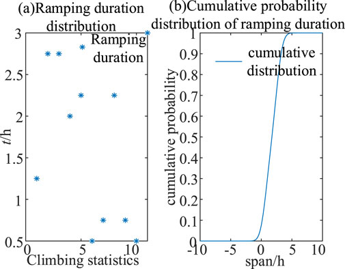
Figure 8. Ramp duration chart. (A) Ramping duration distribution. (B). Cumulative probability distribution of ramping duration.
Figure 8A shows the distribution of ramp length, 12 ramp segments were identified, the shortest segment was 0.5 h, the longest segment was 3 h, and the average time of each segment was 1.8 h. Figure 8B shows the cumulative distribution of continuous time ramp, with more than 90% of the continuous time counted in the area within 2.234 h.
Combined with the previous analysis, the basic flow of this algorithm is given as follows: based on the extraction of extreme value points, the identification of ramp segments is completed.
Step 1. Extract the extreme point of the historical actual power sequence, according to the extreme value extraction method and Equations 3–9 to get the extreme value series E, also known as the TRP series Y.
Step 2. the amplitude change of power, according to C1 of Equation 14 and the TRP sequence calculation statistics, analyzes the cumulative probability distribution of amplitude change by calculation, sets the ramp amplitude threshold limit, and finds out Equation 14.
Step 3. sets the ramp rate threshold and calculates and analyzes the power rate of C2 of Equation 14 and the TRP sequence by calculating and analyzing the cumulative probability distribution of the rate of change.
Step 4. Identify the stationary point based on the stationary point identification condition in Equation 14 Identify the stationary point based on Equations 15, 16 based on the parameters determined by STEP2 and STEP3, and identify the upper and lower ramps based on Equations 15, 17 to count the length of the ramp time.
5 Segmentation prediction algorithm
To improve the performance of wind power prediction under the full-time period and make the model fit the typical characteristics of various meteorological types, this paper proposes a time-series segment prediction algorithm that combines point prediction and probabilistic prediction. Based on the extraction results of meteorological periods in the ramp segment in Section 3, the time series is divided into a fluctuation segment and a low output leveling segment, corresponding to the probability prediction and point prediction respectively. This method helps to improve the reasonableness and readability of the prediction results, and reduces the amount of modeling operations, and improves the computational efficiency.
5.1 LightGBM-LSTM based point prediction method
In practical applications, full-time power prediction challenges a single prediction model. In this paper, a combined LightGBM-LSTM prediction method is proposed to improve the problem of insufficient prediction accuracy in specific scenarios. Massive feature data are used as inputs to the LSTM network and LightGBM prediction model, respectively; meanwhile, to improve the prediction accuracy of the LSTM neural network, the preliminary prediction result of the LightGBM model is input into the LSTM network as one of the features. This combined prediction model can combine the respective features of the above 2 models, which can not only explore the intrinsic connection between multi-feature data but also avoid the bad influence on the prediction accuracy due to over-fitting.
5.1.1 LightGBM model
LightGBM is a framework for implementing the gradient boosting decision tree algorithm. The training speed is faster, the memory consumption is lower, the accuracy is better, the support of distributed, and the fast processing of massive data can be performed (Chen et al., 2021). The main improvements of the LightGBM model include the histogram algorithm and the Leaf-Wise Reading Strategy (Ju et al., 2019). Among them, the former can be substantially reduced in terms of memory usage; the latter can grow deeper decision trees for better prediction accuracy with the same number of breaks. In addition, LightGBM supports category characteristics that do not need to be transformed (e.g., whether it is weather on a ramp road) and incorporates decision rules for category characteristics in the decision tree algorithm.
5.1.2 LSTM
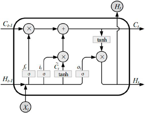
LSTM is a special kind of Recurrent Neural Network architecture (Nguyen. et al., 2024), which can solve the problem of modeling time-series data of integrated drives. LSTM can effectively deal with the long-time dependency relationship and introduces the “memory unit” and gating mechanism. The structure of LSTM is shown in Figure 9.
Figure 9 shows the input
The
The input information for each step of the LSTM contains the
The oblivion gate decides which information of
The computational expression for
Where:
The input gate controls the input information of the current step. It consists of two parts: one part uses a tanh function to filter valid information from
The computational expressions for the
where:
The output gate determines the output information of the current time step, which uses the Sigmoid function to obtain
The computational expressions for the
where:
5.2 Probabilistic prediction methods based on temporal pattern classification
5.2.1 Convolutional neural networks
CNN is a feed-forward neural network type of deep learning model, due to its properties of extracting spatial features commonly used in various data analysis, computer vision, natural language processing, and other fields, so a convolutional layer is set up in the data to extract spatially correlated features. Especially for the characteristics of multi-dimensional extraction of data, to reduce the complexity of the problem; the pooling layer is designed to reduce the dimensionality and number of data so that it can reduce a lot of features that need to be operated to improve the learning efficiency; with the development of deep learning, more and more forms of convolution can be exercised to improve the effect of residual convolution, Alexnet and other convolution of different functions.
5.2.2 Bidirectional gated recurrent unit (Bi-GRU)
GRU uses recursion to obtain global information from the input sequence, utilizes update gate and reset gate to reduce gradient dispersion, and achieves the ability to remember the sequence over time and less computational loss. The update gate determines how much previous information is currently retained at the forecast point.
where:
Reset gate controls how much historical information should be ignored and determines whether the storage unit removes unnecessary detection features. Described as
where:
Effective forecasting models need to extract implicit features and complex changes in serial data. However, GRU can only extract information from the forward direction, while ignoring the valuable information in the backward time series data. Therefore the algorithmic idea of Bi-GRU is proposed, in which the Bi-GRU layer in the encoder consists of two independent GRU networks as shown in Figure 2. They are interconnected at adjacent depths to ensure that the hidden layer state at the previous depth can be transferred to the next hidden state in one direction and features can be extracted from both directions. Bi-GRU can be represented as
where:
6 Calculation validation
6.1 Description of experimental data
Selected for this test sample is information from a wind farm in the country. The data and information of this experiment include the annual output power of this wind farm in 2021 as well as a variety of meteorological factors during the same period. All the above data intervals are 15 min. To verify the effectiveness and superior performance of the algorithm of this paper for the weather conditions of the ramp segment, 10% of the wind farm data of variable meteorological scenarios containing the weather of the ramp segment are specially selected as the validation dataset.
6.2 Evaluation indicators
The article evaluates the prediction performance in terms of both deterministic and uncertainty prediction metrics. Among the deterministic prediction evaluation metrics include relative root mean square error (RRMSE) and mean absolute percentage error (MAPE).
Where: n is the total number of prediction samples;
Uncertainty prediction evaluation metrics include prediction interval coverage percentage (PICP) and prediction interval average width (PINAW) (Ushakov and Ushakov, 2012).
Where:
6.3 Validation of point prediction results
The LIGHTGBM model in the MATLAB platform is used to call the LIGHTGBM machine learning library, the number of weak back trees is 200, the number of leaves is 50, the learning rate is 0.05, and the number of iterations is 3,000; the short-term prediction model of wind power based on the LSTM model constructed by using the KERAS framework. The initialization parameters of the prediction model are: the number of nodes in the hidden layer of the model network and the learning rate of the weights are determined by the IGWO algorithm, the number of model iterations is 15, and the activation function of the LSTM model uses the Sigmoid function.
The data for the training set of the model is the first 80% of the full year 2021 data, while the data for the test set is the last 20%. To observe the prediction effect over a longer time interval, the 2021 data is subjected to several sets of short-term 60-day rolling forecasts with a forecast window of 10 days, i.e., the power changes are predicted 10 days in advance for the next 10 days. As described in 5.1, the algorithm especially selects the power-abrupt time-series segments containing the weather of the ramp segment as the validation dataset and predicts the wind power under the variable meteorological scenarios using LightGBM (Zheng and Kusiak, 2009; Zareipour et al., 2011b), LSTM (Greaves et al., 2009), and LightGBM-LSTM, respectively, and the prediction results of the algorithms are shown in Table 2. The resultant curves are predicted in different ways, as shown in Figure 10.
Comparing the prediction curves in Figure 10, it can be seen that the prediction effect of LightGBM-LSTM algorithm is closer to the real value. And it can be further seen from the prediction errors (RRMSE and MAPE were calculated using Equations 27–28) in Table 2 that it has better performance in both RRMSE and MAPE, indicating that the model not only has high prediction accuracy, but also can capture the features of the data well and give predictions close to the true value. Meanwhile it has better prediction stability and generalization ability to prevent overfitting. The improved LightGBM-LSTM algorithm combines the respective features of LSTM and LightGBM, which can not only mine the intrinsic connection between multi-featured data, but also avoid the adverse effects of overfitting, and improve the prediction accuracy of the method by combining the prediction strategies. The LightGBM model has an obvious advantage in prediction speed, but its training process is susceptible to overfitting, which results in a lower prediction accuracy is low. The LSTM network in the combined prediction model adds LightGBM as one of the input feature tensors, and thus has a better prediction effect.
6.4 Analysis of inter-area prediction results
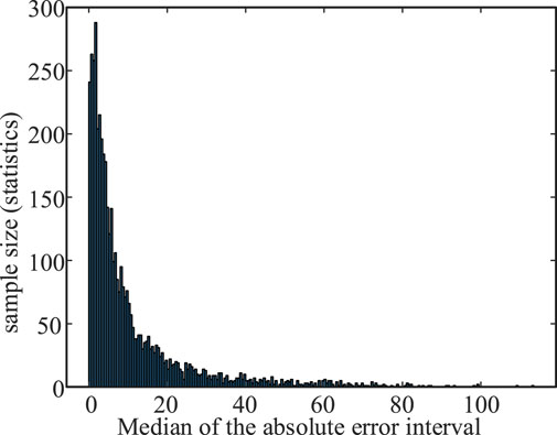
The data of a wind farm with an installed capacity of 201 MW in China is selected for example analysis. Figure 11 shows the distribution of prediction error, and Figure 12 shows the prediction effect of a certain 5-day period in 2021, which shows that the interval prediction model can closely follow the trend of the wind power series under the same confidence level, and obtains a narrower average bandwidth and a higher interval coverage. It can provide more accurate forecast information for decision-makers.
The probabilistic prediction effect is shown in Figure 12, where the probabilistic prediction performance is portrayed through the PICP (Equation 29) and PINAW (Equation 30) evaluation metrics, respectively. It can be seen that the actual power timeseries curve is surrounded by the estimated confidence interval. According to the performance effect of prediction, the model is better able to extract and recognize the transitive time period timing pattern. Obviously, for the probabilistic prediction time period, the prediction intervals of lower confidence intervals are surrounded by higher confidence intervals, which effectively avoids the intersection of quartiles and proves that the power prediction method proposed in this paper has a good comprehensive performance. Further, the CNN-BiGRU-KDE probabilistic prediction method proposed in this paper shows certain accuracy advantages in the 80%, 85%, and 90% confidence intervals, which further demonstrates the effectiveness and superiority of the method proposed in this paper. Meanwhile, it can obtain interval coverage greater than the preset confidence level at different confidence levels. And the probabilistic prediction method based on CNN-BiGRU-KDE not only produces favorable bias at all confidence levels, but also has high reliability.
Based on the above analysis of the deterministic prediction results, it is easy to see that the LightGBM-GRU algorithm adopted in this paper shows a high prediction effect in the small fluctuation and gentle power period. However, for the weather segments with violent fluctuations and ramp segments, there is still a certain error. Especially, it is more obvious in the period of frequent large waves, so the point prediction-probability interval prediction segmentation method proposed in this paper can better make up for the above shortcomings. On the other hand, the probabilistic prediction results are shown as the upper and lower bounds of the confidence interval and the probability density distribution, and the accuracy of the point prediction is sufficient to support the actual demand in the non-ramp weather segments. This is a further manifestation of the rationality of the segmented prediction strategy proposed in this paper. As can be seen from the presentation of the segmented prediction results in Figure 12 above, the actual power time series curve is surrounded by the estimated confidence interval. According to the predicted performance results, the model can extract and recognize the ramp segment period timing patterns better. The prediction intervals of lower confidence intervals are surrounded by higher confidence intervals, which effectively circumvents the interquartile crossover against the probabilistic prediction periods, proving that the comprehensive performance of the power prediction approach mentioned in this paper is good.
7 Conclusion
This paper proposes a short-term wind power segmentation prediction method based on the identification of ramp segment periods for the phenomenon of sudden power change in a short period of time under climbing segment meteorology. Compared with the existing methods, the proposed method improves the efficiency and accuracy of fluctuating period extraction in the ramp segment through the adaptive turning time period identification method based on local feature distribution; the improved LightGBM-LSTM algorithm can not only mine the intrinsic connection between multi-feature data, but also avoid the adverse effect of overfitting, and improve the prediction accuracy through the combination of prediction strategies; the proposed CNN-BiGRU-KDE probabilistic prediction method shows good prediction performance at the specified confidence level; by proposing a segmented prediction method based on the temporal pattern, it overcomes the influence of the variability of the power temporal features on the prediction results under the meteorological model, and significantly improves the model prediction performance. In summary, the prediction method proposed in this paper has good prediction accuracy in the full time period including the ramp segment weather, and has good generalization performance, which provides a certain useful supplement for the research in the field of ultra-short-term wind power prediction.
Data availability statement
The original contributions presented in the study are included in the article/supplementary material, further inquiries can be directed to the corresponding author.
Author contributions
CY: Writing–review and editing, Writing–original draft, Methodology, Investigation, Funding acquisition, Formal Analysis. GW: Writing–original draft, Writing–review and editing, Methodology, Investigation, Funding acquisition, Data curation. YZ: Visualization, Resources, Writing–review and editing, Supervision. GB: Visualization, Writing–review and editing, Supervision, Funding acquisition. JW: Writing–review and editing, Supervision.
Funding
The author(s) declare that financial support was received for the research, authorship, and/or publication of this article. This work was supported in part by the Science and Technology Project of State Grid Gansu Electric Power Company Electric Power Science Research Institute under Grant (No. SGGSKY00WYJS2310221).
Conflict of interest
Authors CY and GW were employed by Power Dispatch Center of State Grid Gansu Electric Power Company. Author YZ was employed by Electric Power Science Research Institute of State Grid Gansu Electric Power Company.
The remaining authors declare that the research was conducted in the absence of any commercial or financial relationships that could be construed as a potential conflict of interest.
The authors declare that this study received funding from Electric Power Scientific Research Institute of State Grid Gansu Power Company. The funder had the following involvement in the study: the collection and analysis of the data, as well as the funder’s decision to submit the article for publication.
Publisher’s note
All claims expressed in this article are solely those of the authors and do not necessarily represent those of their affiliated organizations, or those of the publisher, the editors and the reviewers. Any product that may be evaluated in this article, or claim that may be made by its manufacturer, is not guaranteed or endorsed by the publisher.
References
Cassola, F., and Burlando, M. (2012). Wind speed and wind energy forecast through Kalman filtering of numerical weather prediction model output. Appl. Energy 99 (6), 154–166. doi:10.1016/j.apenergy.2012.03.054
Chen, W., Hu, Z., Yue, J., et al. (2021). Short-term load prediction based on combined model of long short-term memory network and light gradient boosting machine. Automation Electr. Power Syst. 45 (4), 91–97. (in Chinese).
Cheng, L., and Yu, T. (2019). A new generation of AI: a review and perspective on machine learning technologies applied to smart energy and electric power systems. Int. J. Energy Res. 43 (6), 1928–1973. doi:10.1002/er.4333
Cui, M., Sun, Y., and Ke, D. (2014). Prediction of wind power ramp based on sparse decomposition of atoms and BP neural network. Automation Electr. Power Syst. 38 (12), 6–11. (in Chinese).
Cui, M., Zhang, J., Wang, Q., Krishnan, V., and Hodge, B. M. (2019). A data-driven methodology for probabilistic wind power ramp forecasting. IEEE Trans. Smart Grid 10 (2), 1326–1338. doi:10.1109/tsg.2017.2763827
Cutler, N., Outhred, H., and Macgill, I. (2011). Final report on UNSW Project for AEMO to develop a prototype wind power forecasting tool for potential large rapid changes in wind power. Univ. N. S. W Centre Energy Environ. Mark.
Erdem, E., and Shi, J. (2011). ARMA based approaches for forecasting the tuple of wind speed and direction. Appl. Energy 88 (4), 1405–1414. doi:10.1016/j.apenergy.2010.10.031
Ernst, B., Oakleaf, B., Ahlstrom, M., Lange, M., Moehrlen, C., Lange, B., et al. (2007). Predicting the wind. IEEE Power Energy Mag. 5 (6), x5–x78. doi:10.1109/mpae.2007.4317489
Ferreira, C., Gama, J., Matias, L., et al. (2011). A survey on wind power ramp forecasting. Rep. ANL/DIS-10-13, Argonne Natl. Lab.
Freedman, J., Markus, M., and Penc, R. (2008). Analysis of West Texas wind plant ramp-up and ramp-down events. New York: AWS Truewind.
Gao, Y., Qu, C., and Zhang, K. (2016). A hybrid method based on singular spectrum analysis, firefly algorithm, and BP neural network for short-term wind speed forecasting. Energies 9 (10), 757. doi:10.3390/en9100757
Greaves, B., Collins, J., Parkes, J., and Tindal, A. (2009). Temporal forecast uncertainty for ramp events. Wind Eng. 33 (33), 309–319. doi:10.1260/030952409789685681
Haoyi, X., Xiaoxia, H., and Chunli, L. (2023). Probability density forecasting of wind power based on transformer network with expectile regression and kernel density estimation. Electronics 12 (5), 1187. doi:10.3390/electronics12051187
Hu, Q., Zhang, S., Xie, Z., Mi, J., and Wan, J. (2014). Noise model based νν-support vector regression with its application to short-term wind speed forecasting. Neural Netw. 57 (9), 1–11. doi:10.1016/j.neunet.2014.05.003
Huang, Q., Wang, Z., Du, B., et al. (2016). Research on wind power grade ability prediction based on pre-decomposition combined forecasting. Renew. Energy 34 (12), 1847–1852. (in Chinese).
Jianhou, W., Yue, Y., Bo, Z., and Lu, H. (2024). Hybrid ultra-short-term PV power forecasting system for deterministic forecasting and uncertainty analysis. Energy 288, 129898. doi:10.1016/j.energy.2023.129898
Ju, Y., Sun, G., Chen, Q., Zhang, M., Zhu, H., and Rehman, M. U. (2019). A model combining convolutional neural network and LightGBM algorithm for ultra-short-term wind power forecasting. IEEE Access 7, 28309–28318. doi:10.1109/access.2019.2901920
Kamath, C. (2010). “Understanding wind ramp events through analysis of historical data,” in PES transmission and distribution conference and exposition (New Orleans, USA: IEEE), 1–6.
Kamath, C. (2011). “Associating weather conditions with ramp events in wind power generation,” in Power Systems Conference and Exposition, Phoenix, AZ, USA, 20-23 March 2011 (IEEE), 1–8.
Lefeng, C., Guiyun, L., Hanqi, Hu., Wang, X., Chen, Y., Zhang, J., et al. (2020). Equilibrium analysis of general N-population multi-strategy games for generation-side long-term bidding: an evolutionary game perspective. J. Clean. Prod. 276, 124123. doi:10.1016/j.jclepro.2020.124123
Lefeng, C., Linfei, Y., Jianhui, W., et al. (2021). Behavioral decision-making in power demand-side response management: a multi-population evolutionary game dynamics perspective. Int. J. Electr. Power Energy Syst., 129.
Lefeng, C., Yang, C., and Guiyun, L. (2022). 2PnS-EG: a general two-population n-strategy evolutionary game for strategic long-term bidding in a deregulated market under different market clearing mechanisms. Int. J. Electr. Power and Energy Syst. 142 (A), 108182. doi:10.1016/j.ijepes.2022.108182
Li, C. (2013). Moving average trading strategies effectiveness research. Shanghai Jiao Tong Univ. (in Chinese).
Liu, R., Shi, J., Sun, G., Lin, S., and Li, F. (2024). A Short-term net load hybrid forecasting method based on VW-KA and QR-CNN-GRU. Electr. Power Syst. Res. 232, 110384. doi:10.1016/j.epsr.2024.110384
Men, Z., Yee, E., Lien, F., Wen, D., and Chen, Y. (2016). Short-term wind speed and power forecasting using an ensemble of mixture density neural networks. Renew. Energy 87 (3), 203–211. doi:10.1016/j.renene.2015.10.014
Meng, A., Chen, S., Wang, C., et al. (2021). Ultra-short-term wind power prediction based on chaotic CSO optimized temporal attention GRU model. Power Syst. Technol. 45 (12), 4692–4700. (in Chinese).
Nguyen., B. N., E, O., E, P., Alberti, D., Leva, S., and Duong, M. Q. (2024). “Forecasting generating power of sun tracking PV plant using long-short term memory neural network model: a case study in ninh thuan – Vietnam,” in 2024 Tenth International Conference on Communications and Electronics (ICCE), Danang, Vietnam, 31 July 2024, 333–338. doi:10.1109/icce62051.2024.10634629
Ouyang, T., Huang, H., and He, Y. (2019). Ramp events forecasting based on long-term wind power prediction and correction. IET Renew. Power Gener. 13 (15), 2793–2801. doi:10.1049/iet-rpg.2019.0093
Ouyang, T., Zha, X., Qin, L., et al. (2017). Wind power ramp events forecast method based on similarity correction. Proc. CSEE 37 (2), 572–580. (in Chinese).
Potter, C., Grimit, E., and Niissen, B. (2009). Potential benefits of a dedicated probabilistic rapid ramp event forecast tool. Power Syst. Conf. and Expo. 107 (1), 1–5. doi:10.1109/psce.2009.4840109
State Grid (2021). State Grid Corporation of China issues “carbon peak and carbon neutrality” action plan. State Grid Rep., 001. (in Chinese).
Truewind, A. W. S. (2008). AWS True wind’s final report for the Alberta forecasting pilot project. Wind Power Forecast. PILOT Proj.
Ushakov, N. G., and Ushakov, V. G. (2012). On bandwidth selection in kernel density estimation. J. Nonparametric Statistics 24 (2), 419–428. doi:10.1080/10485252.2012.655734
Wang, M., Ying, F., and Nan, Q. (2024). Refined offshore wind speed prediction: leveraging a two-layer decomposition technique, gated recurrent unit, and kernel density estimation for precise point and interval forecasts. Eng. Appl. Artif. Intell. 133 (PE), 108435. doi:10.1016/j.engappai.2024.108435
Wang, Y., Gao, S., Jia, W., Ding, T., Zhou, Z., and Wang, Z. (2022). Data-driven distributionally robust economic dispatch for park integrated energy systems with coordination of carbon capture and storage devices and combined heat and power plants. IET Renew. power Gener. 16 (12), 2617–2629. doi:10.1049/rpg2.12436
Zareipour, H., Huang, D., and Rosehart, W. (2011a). Wind power ramp events classification and forecasting: a data mining approach. Detroit, USA: IEEE Power and Energy Society General Meeting.
Zareipour, H., Huang, D., and Rosehart, W. (2011b). Wind power ramp events classification and forecasting: a data mining approach. San Diego, IEEE: IEEE Power and Energy Society General Meeting, 1–3.
Zhang, D., Dai, Y., Zhang, X., et al. (2018). Review and prospect of research on wind power ramp events. Power Syst. Technol. 42 (6), 1783–1792. (in Chinese).
Zheng, H., and Kusiak, A. (2009). Prediction of wind farm power ramp rates: a data-mining approach. J. Sol. Energy Eng. 131 (3), 376–385. doi:10.1115/1.3142727
Keywords: ramp segment, wind power, trend identification, probabilistic fitting, segmental prediction
Citation: Yang C, Wu G, Zhang Y, Bao G and Wang J (2024) A study of short-term wind power segmentation forecasting method considering weather on ramp segments. Front. Energy Res. 12:1474969. doi: 10.3389/fenrg.2024.1474969
Received: 02 August 2024; Accepted: 25 September 2024;
Published: 16 October 2024.
Edited by:
Yang Yu, Nanjing University of Posts and Telecommunications, ChinaReviewed by:
Minh Quan Duong, The University of Danang, VietnamLefeng Cheng, Guangzhou University, China
Copyright © 2024 Yang, Wu, Zhang, Bao and Wang. This is an open-access article distributed under the terms of the Creative Commons Attribution License (CC BY). The use, distribution or reproduction in other forums is permitted, provided the original author(s) and the copyright owner(s) are credited and that the original publication in this journal is cited, in accordance with accepted academic practice. No use, distribution or reproduction is permitted which does not comply with these terms.
*Correspondence: Chunxiang Yang, MjA3MTc2MzM4NUBxcS5jb20=
 Chunxiang Yang1*
 Jianhui Wang