 Xiaorui Liang
 Huaying Zhang1*
 Qian Liu
- 1New Smart City High-Quality Power Supply Joint Laboratory of China Southern Power Grid, Shenzhen Power Supply Co., Ltd., Shenzhen, Guangdong, China
- 2College of Electrical and Information Engineering, Hunan University, Changsha, Hunan, China
In distribution networks with distributed generators (DGs), power generation and load demand exhibit increased randomness and volatility, and the line parameters also suffer more frequent fluctuations, which may result in significant state shifts. Existing model-driven methods face challenges in efficiently solving uncertain power flow, especially as the size of the system increases, making it difficult to meet the demand for rapid power flow analysis. To address these issues, this paper proposes an SVR-based interval power flow (IPF) prediction method for distribution networks with DGs integration. The method utilizes intervals to describe system uncertainty and employs Support Vector Regression (SVR) for model training. The input feature vector consists of the intervals of active power generation, load demand, and line parameters, while the output feature vector represents the intervals of voltage or line transmission power. Ultimately, the SVR-based IPF prediction model is established, capturing the linear mapping relationship between input data and output IPF variables. Simulation results demonstrate that the proposed method exhibits high prediction accuracy, strong adaptability, and optimal computation efficiency, meeting the requirements for rapid and real-time power flow analysis while considering the uncertainty in distribution networks with DGs integration.
1 Introduction
1.1 Motivation
In the context of widespread integration of distributed generators (DGs) such as wind and photovoltaic (PV) power into distribution networks, power generation exhibits uncertainty due to the inherent volatility and randomness of wind and solar. In addition, load demand and line parameters also exhibit uncertainty which is caused by user consumption behaviors and environmental factors, respectively. These issues caused the power flow state in the system to undergo rapid and intricate changes. Considering these uncertainties, uncertain power flow (PF) methods are proposed by researchers. However, most existing uncertain PF methods are model-driven. As the system scale increases, the model complexity grows, leading to a significant reduction in computational efficiency, which fails to meet the requirements for rapid assessment of system states in distribution networks. Improving the computational efficiency of uncertain PF analysis can provide assurance for real-time monitoring and dispatching of distribution systems, ensuring stable and efficient operation. There is an urgent need for efficient and rapid methods for uncertain PF analysis in distribution networks that can effectively address system uncertainty.
1.2 Focus and potential
This paper focuses on addressing the computational efficiency issues of uncertain PF, primarily in two aspects: describing system uncertainty using intervals and employing data-driven methods for PF prediction, enabling real-time interval power flow (IPF) calculations in distribution systems. The potential of this research lies in its ability to significantly enhance the real-time monitoring and operational capabilities of distribution networks with integrated DGs. By addressing the limitations of existing model-driven uncertain PF methods, the proposed approach could lead to more efficient PF analysis, particularly in the face of the increasing penetration of renewable energy sources (RES). This has offered a scalable solution for real-time PF analysis in increasingly complex and uncertain environments.
1.3 Preceding research
Commonly used methods for handling uncertainty currently include robust, probabilistic, and interval methods. Among them, the robust method is mainly used for optimization (Zheng et al., 2024), such as energy management under the uncertainty of renewable energy generation and electric vehicles (EVs) (Tan et al., 2024). When calculating power flow, the probabilistic method and interval algorithm are more frequently employed, which are called probabilistic power flow (PPF) and interval power flow (IPF). IPF has the advantages of simple modelling and high security compared with PPF. Existing IPF methods primarily consist of iterative approaches (Mori and Yuihara, 1999; Barboza et al., 2004) and optimization techniques (Zhang et al., 2017; 2018; 2023). For iterative approaches, the Interval Newton iteration was first employed. To avoid solving the equations in the Interval Newton method, the Krawczyk method was introduced. The interval problem was broken down into multiple sub-intervals, and each sub-interval was solved iteratively using the Krawczyk method (Mori and Yuihara, 1999). The Interval Newton iteration framework was combined with the Krawczyk operator in (Barboza et al., 2004), enhancing convergence performance. The introduction of the Affine Algorithm (AA) (Vaccaro et al., 2010) increased the efficiency and accuracy of solving interval nonlinear equation systems. The convergence of the Krawczyk-Moore iteration was enhanced by introducing AA, and the correlation issues of interval computation were addressed. Optimization methods, which avoid iteration and convergence problems, have gained widespread attention in recent years. The optimization model for the IPF solution was constructed by converting intervals into affine forms (Zhang et al., 2017), improving the efficiency of solving IPF. An optimization scenario method (OSM) was improved to solve IPF (Zhang et al., 2018), directly obtaining the range of power flow variables through the optimization models. In IPF analysis for distribution networks, the rise of AA has led to a trend of combining it with the Distflow model, including solving the affine Distflow model using forward-backward substitution (Cheng et al., 2023; Lyu et al., 2023) and directly establishing AA-based IPF optimization models (Leng et al., 2020; Cao et al., 2024). However, existing uncertainty analysis based on physical models suffers from the drawback of increased computational complexity, resulting in lengthy processing times, making it challenging to meet the power grid’s demand for swift power flow computations.
Due to the advancements in computer and digital communication technologies, data acquisition in power systems has made significant progress. The deployment of Wide Area Measurement Systems (WAMS) has enabled the reliable collection of high-precision, wide-area synchronized electrical quantities, including voltage, current, phase angles, et al. This progress has fostered the development of data-driven power flow analysis methods, providing a solution to the issue of low efficiency in traditional model-driven power flow analysis (Fu et al., 2024). A data-driven linear PF model incorporating the support vector regression (SVR) and ridge regression (RR) algorithms was proposed in (Li et al., 2023). Similarly, a linear regression model was solved by RR to suppress the effect of data collinearity in (Chen, Y. et al., 2022). In distribution networks, the single-phase PF model is often considered. For instance, a data-driven single-phase linear PF model was introduced in (Xing et al., 2021). A data-driven convex model for hybrid AC/DC microgrids operation involving bi-directional converters was proposed in (Liang et al., 2023). Nevertheless, distribution power systems (DPSs) are generally unbalanced and it is still necessary to study linear three-phase distribution PF models. A data-driven-aided linear three-phase PF model for DPSs considering the imbalance was constructed in (Liu, Y. et al., 2022), and a data-driven piecewise linearization for distribution three-phase stochastic power flow was proposed in (Chen, J. et al., 2022), mitigating the errors of model-based PF linearization approaches. To overcome the challenge of obtaining accurate results with linear model-based data-driven methods, an approach with high adaptability to the nonlinearity of PF was proposed based on the thought of Koopman operator theory (Guo et al., 2022). What’s more, a risk-free method was proposed in (Dong et al., 2022) to accelerate AC power flow with machine learning-based initiation, reducing the PF computation time. To tackle the challenges of the hidden measurement noise in the data-driven PF linearization, the problem was transformed into a regression model where the structure of the PF equations was exploited (Liu et al., 2020). Besides, the local load fluctuation suppression and its interaction with distribution system should also be addressed which brings the exact necessity towards the power flow prediction (Khalid et al., 2022; Rehman et al., 2024). Also, here the role of ancillary services and renewable energy integration should also be addressed towards covering the intermittency (Musleh et al., 2019; Sun et al., 2020). In some cases, the database may not possess the envisioned completeness and appropriateness. There is a trend that combines the physical model-driven and data-driven. This can make up for the issues arising from incomplete data (Xing et al., 2022; Liu et al., 2021). A hybrid physical model-driven and data-driven approach for linearizing the power flow model was proposed in (Tan et al., 2020), and the linearized errors are obtained by the partial least squares regression-based data-driven approach. In the condition of lack of data, physical model parameters are introduced to assist the data-driven training process (Shao et al., 2023), and a highly scalable data-driven algorithm for stochastic AC-OPF that has extremely low sample requirements was presented in (Mezghani et al., 2020). To enhance the performance and generalization ability of the data-driven model, a physics-guided neural network was proposed to solve the PF problem by encoding different granularity of Kirchhoff’s laws, and system topology into the rebuilt PF model (Hu et al., 2021). The fusion of robust principles with data-driven approaches has also enhanced the precision of data-driven methods. The worst-case errors were probabilistically constrained through distributionally robust chance-constrained programming (Liu, Y. et al., 2022; Chen et al., 2020). It also allows guaranteeing the linearization accuracy for a chosen operating point. In addition, a more comprehensive summary and discussion of existing data-driven PF linearization was presented in (Jia and Hug, 2023). For data-driven methods, support vector machine (SVM) is widely used due to its strong robustness and generalization ability, particularly excelling in scenarios with small samples and high dimensionality. Addressed to the N-k1-k2 cascading outages, the researchers employ SVM for classifier training, enabling the fast, reliable, and robust computation of active and reactive power flows (Xue and Liu, 2021). The SVM is utilized for optimal power flow with small-signal stability constraints in (Liu, J. et al., 2022), achieving high computational efficiency and economic benefits.
Although data-driven PF methods have made significant advancements, combining data-driven approaches with uncertainty still presents challenges. On the one hand, data-driven methods require a large amount of real or simulated data, which is what uncertain PF lacks. Historical data is difficult to obtain, and generating simulated data often incurs higher costs compared to deterministic PF. On the other hand, effectively integrating uncertainty into data-driven models is a challenge, as these uncertainties are often high-dimensional, increasing the complexity of modeling. In response, interval approaches offer the advantages of simple modeling and high simulation accuracy, while SVR can handle high-dimensional data, making it suited to the requirements. Therefore, this paper adopts interval modeling to represent uncertainties and selects SVR as the data-driven approach.
1.4 Contribution
This paper is dedicated to improving the computational efficiency of IPF in distribution networks to achieve real-time analyses, providing essential support for the rapid response of uncertain distribution systems with DGs integration. To this end, a method for IPF prediction in distribution networks based on SVR is proposed by combining data-driven methods with interval approaches. Accordingly, the research makes the following contributions.
Firstly, an IPF model for distribution networks based on the OSM is established considering system uncertainty as intervals. In addition to the uncertainty of power generation and load demand, the uncertainty of line parameters is also considered in this model. Due to environmental variations, the parameters of network lines exhibit a certain level of uncertainty. This consideration improves the accuracy of the model.
Secondly, an IPF prediction model is constructed using SVR based on the interval dataset generated by simulation. Different from traditional data-driven models, this model is a multi-output model that separately outputs the upper and lower bounds of the power flow results. This interval result fully considers various uncertainties in the distribution system, as the model is trained with these uncertainties incorporated.
Thirdly, the established SVR-based IPF prediction approach has been demonstrated to have high prediction accuracy and computational efficiency. The effectiveness of this approach is validated through studies on both IEEE 33bw and IEEE 69 cases. The IEEE 33bw case is primarily used to evaluate the model’s accuracy, while the IEEE 69 case is mainly used to analyze the model’s computational efficiency.
The IPF model for distribution networks is introduced in Section 2. The training and prediction algorithm through SVR is introduced in Section 3. The procedure of the method is introduced in Section 4. The case studies are conducted in Section 5, and conclusions in Section 6.
2 Construction of IPF model for distribution networks
2.1 Distflow formulation
The relaxed Distflow model for the radial distribution network is expressed as Equations 1–4. Before constructing the model, it is customary to assume that the transmission lines do not involve parallel grounding branches and to specify that the direction of current and power flow from node i to node j is positive.
The model is the branch power flow model after convex relaxation, where Equation 1 is the voltage equation, Equation 2 is the power equation at the sending end of the branch, Equations 3, 4 are the power balance equation.
2.2 Modelling of IPF based on distflow
In active distribution networks with DGs integration, the output of distributed generators and flexible loads both exhibit a certain degree of uncertainty, which has a significant impact on the safe and stable operation of the distribution networks. Therefore, it is essential to consider these uncertainties. In this paper, the interval approach is utilized to describe uncertainties, ensuring the security of system operation. Additionally, the network parameters, including line resistance and reactance, may experience variations due to external environmental factors. To make the model more practical, the uncertainties of these parameters are considered simultaneously during modelling.
In the interval approach, the active power generation and load demand, as well as line parameters are represented in interval form, and the interval results for variables such as voltage and line transmission power can be obtained. Representing the interval form in
where
The IPF model based on Distflow can draw inspiration from the principles of OSM for its solution. In this approach, the interval uncertainties of the IPF model are regarded as variables that vary in their interval bounds, and the desired variables are set as the objective functions. Thus, it involves transforming the resolution of a set of interval nonlinear equations into variable optimization problems. The core of OSM is based on the Extreme Value Theorem through which we can get two points of conclusions. We simplify Equations 5–8 as
From the two points of conclusions, the solution for IPF model is reduced to find
Taking the variable
It can be succinctly described as searching for a specific scenario
3 IPF prediction method for distribution networks based on SVR
As the system scale increases, the efficiency of model-driven IPF analysis significantly decreases, which does not meet the current demands for rapid PF computations in distribution networks. Therefore, the data-driven approach has garnered attention for achieving faster IPF computations. The SVR has been opted for in this research due to its advantages of handling high-dimensional data, which is aligned with the characteristics of IPF analysis.
3.1 Construction of eigenvectors in IPF
In the typical SVR framework, the model is designed for single-output problems. However, in the context of IPF models, situations may arise where some nodes attain their maximum values while others reach their minimum values within the same input scenario since both input data and output variables are represented as intervals. Therefore, the SVR model for IPF is fundamentally a multiple-output problem. Corresponding to the same input scenario, the situation where different nodes attain either maximum or minimum values may vary. In such cases, training the SVR model based on the specific input and a singular minimum (or maximum) output would lead to a significant decrease in model accuracy. Based on this, the feature vectors in IPF model are established.
The well-constructed feature vectors are crucial prerequisites for ensuring the effectiveness of data-driven model learning. In the analysis of extensive historical state data for distribution networks with DGs, it is essential to determine the input and output features for the IPF analysis at first. Given that the primary characteristic of distribution networks with DGs is the uncertainty of renewable power generation and load demand, which significantly impacts IPF analysis results, the sequence of renewable power generation and load demand for the distribution system is selected as the input eigenvector of the SVR model, and the sequence of node voltages and active line transmission power, which is indicative of power flow results, is selected as the output feature vector.
3.1.1 Construction of input eigenvector adapted to variations in source-grid-load
The uncertainty of source, grid, and load is represented in interval form for the IPF model. Therefore, the values in the input eigenvector should be intervals distinguishing from conventional eigenvectors. However, directly using interval values for training poses challenges such as computational complexity, model misfit, and difficulty in interpreting learning patterns. To address these issues, it is necessary to identify relevant parameters that can characterize interval features, such as interval midpoints and interval radii, to replace interval values during training. The midpoint of the interval is the operating point of generator, which reflects the randomness of generator output. The interval radius can reflect the fluctuation degree of uncertain data. Therefore, the interval midpoint of source and radius of source-grid-load data is used to construct the input eigenvector instead of interval values.
Take the renewable active power generation
where
The eigenvector for source includes the sequence of renewable active power generation
where M is the number of DGs,
3.1.2 Construction of output feature vector
When conducting PF analysis, it is essential to consider the output features that can reflect power system quality and stability. In power flow results, node voltage or line transmission power can be used to evaluate system stability. Therefore, the node voltage is selected as output features in this paper. In IPF model, node voltages are represented as interval values, so that the output features of the SVR training model are essentially intervals. However, training the model directly with interval values as the output vector may lead to issues such as model complexity and low interpretability. To address the issues, it is preferable to choose upper and lower bounds that characterize interval features as the output feature vector. This involves establishing the SVR model with two output nodes. According to this, the output feature vector in IPF can be constructed as Equation 14.
Certainly, we can also construct the output feature vector as presented in Equation 15 to obtain the predictive results of line transmission power.
3.2 Modelling of SVR-based IPF prediction
Support Vector Machine (SVM) is a binary classification algorithm, and its fundamental model is a linear classifier that maximizes the margin in the feature space. The objective of SVM learning is to find a hyperplane that separates the samples, guided by the principle of maximizing the margin. This ultimately translates into solving a convex quadratic programming problem. The variant of SVM used in this research for IPF prediction is SVR, specifically designed for solving regression problems. The principle of SVR is presented in Figure 1. SVR can be categorized into three types according to the linear separability of the training data, including Linear Hard ε-SVR, Linear ε-SVR, and ε-SVR.
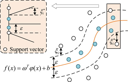
Figure 1. The principle of SVR.
The original data for IPF analysis is considered linearly non-separable. Therefore, this paper selects the ε-SVR model to explore the connection between the input and output of the IPF for distribution systems. Based on the constructed feature vectors in IPF, the ε-SVR model for IPF prediction is established as follows.
According to the description in 3.1, the training data set of the model can be obtained as
where
3.3 Solving of SVR-based IPF prediction model
The SVR training models are solved in this section. To reduce the complexity of solving, the models Equations 16, 17 can be transformed into Equations 18, 19 through applying the Lagrangian function and choosing an appropriate kernel function
where
The structure of SVR training model for IPF prediction can be depicted as shown in Figure 2.
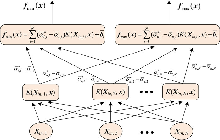
Figure 2. The structure of SVR training model for IPF prediction.
According to Figure 2, the minimum and maximum values of the power flow results, that is the interval results
4 The procedure of SVR-based IPF prediction method
In the SVR-based IPF prediction method for distribution networks, the first step involves establishing an IPF model for generating the initial sample database through simulation. The database includes intervals for node injections of active and reactive power, intervals for line parameter fluctuations, and corresponding intervals for node voltage. The data are then processed to construct the input and output feature vectors. Subsequently, the SVR training model is established, and the formulation of linear decision function can be determined by solving the model. Finally, when given a specific input eigenvector, the interval results for power flow variables can be predicted according to the decision function. The detailed procedure of SVR-based IPF prediction is expressed as follows and the flow chart is presented in Figure 3.
Step1. Data Generating. Generate a diverse set of initial samples according to the established IPF model Equations 5–8 through simulation, where each set comprises the interval of active and reactive node power injection fluctuations, the interval of line parameter fluctuations, and the associated node voltage intervals.
Step2. Data Preprocessing. Select and extract features from the initial samples, and construct the input and output feature vectors Equations 13, 14 for each set of data in the database according to Section 3.1. To ensure the accuracy of model training, normalize the input data. Then select 80% of the database as the training set and 20% of the database as the testing set.
Step3. IPF Prediction Model Construction. Set the parameters
Step4. IPF Prediction Model Solving. Transform the constructed models Equations 16, 17 into Equations 18, 19, and the parameters
Step5. Model Evaluation. Based on the testing dataset, evaluate the performance of the model using appropriate metrics, such as mean absolute error (MAE) and root mean square error (RMSE). Then determine if the metrics meet the requirements. If the metrics meet the expectations, proceed to step6; otherwise, adjust the parameters
Step6. Interval Power Flow Prediction. Give the independent and specific input eigenvector
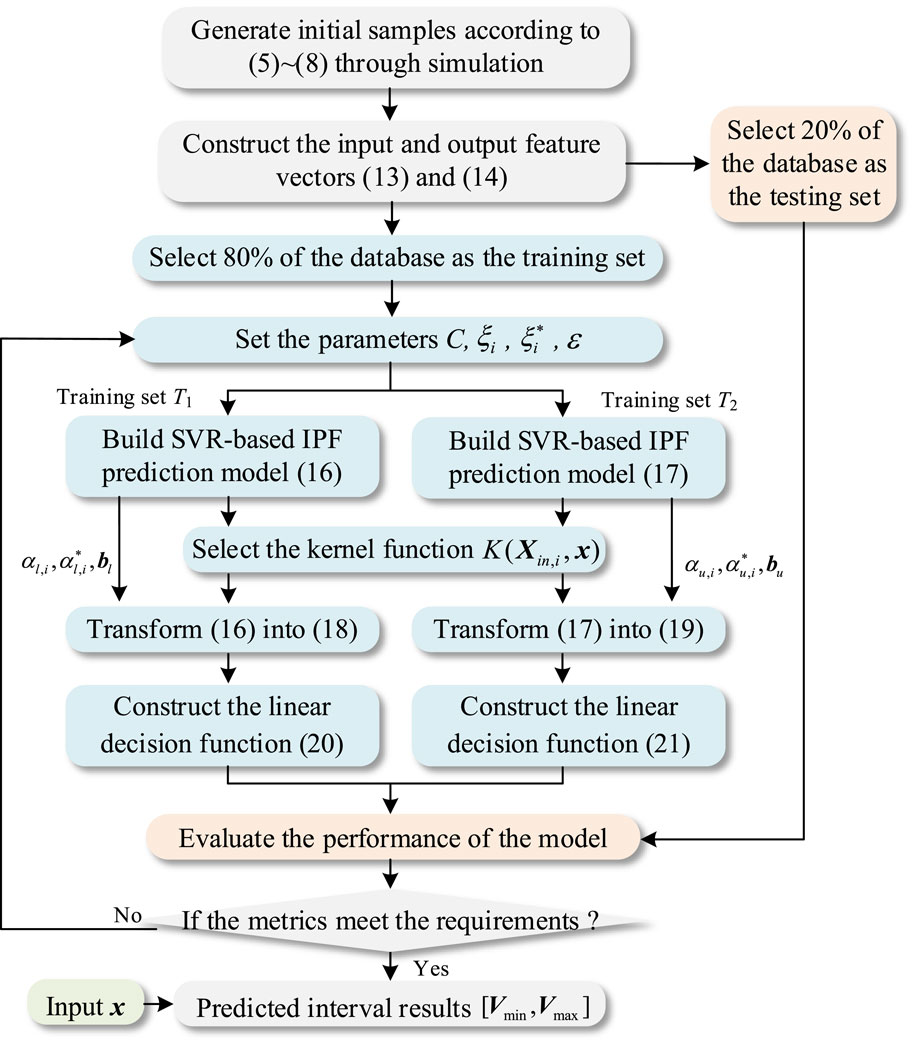
Figure 3. The flow chart of SVR-based IPF prediction method.
5 Case studies
The performance of the proposed SVR-based IPF prediction method is tested on IEEE 33bw and IEEE 69 distribution networks on an Intel(R) Core(TM) i5 PC, 2.50 GHz processor with 8 GB RAM. The algorithm is implemented in MATLAB. The IEEE 33bw case is primarily used to validate the accuracy of the established IPF prediction model and its adaptability to various system fluctuations. Meanwhile, the IEEE 69 case is employed to verify the efficiency and real-time capability of the proposed algorithm in predicting IPF of the distribution network.
5.1 IEEE 33bw case study
The IEEE 33bw case is illustrated in Figure 4, and the case has been enhanced to include eight distributed renewable energy sources. All parameters are valued according to the per unit (p.u.) system of analysis, with 10 MVA chosen as the basic power of the test case. The detailed original power generation data for these eight DGs are presented in Table 1. The voltage limits of all buses except the slack bus are constrained to [0.9,1.1].
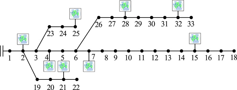
Figure 4. The topology of enhanced IEEE 33bw distribution network.
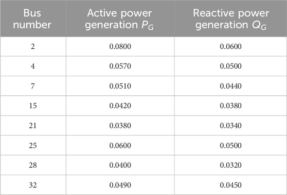
Table 1. The original power generation data of DGs for IEEE 33bw case (p.u.).
5.1.1 Evaluation of the model
The active power generation fluctuation ranges of DGs are assumed to be ±20% of the original data, which is also assumed on the active and reactive load demand, that is the set the fluctuation coefficient
To evaluate the model’s performance comprehensively and objectively, the indices of mean absolute error (MAE), root mean square error (RMSE), mean absolute percentage error (MAPE) and R2 for the testing sets are calculated in this paper. They are defined as Equations 24–27. Using these metrics together helps to avoid biases introduced by a single metric, enhancing the robustness of the evaluation.
where n is the number of samples,
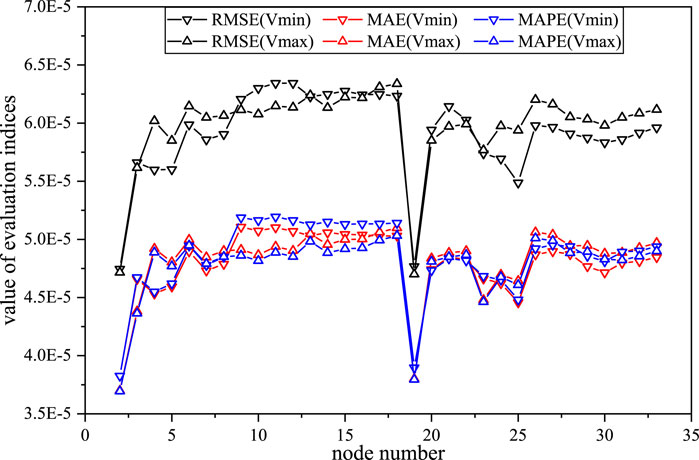
Figure 5. The evaluation results of RMSE, MAE and MAPE for the SVR-based IPF prediction model.
It can be observed from Figure 5 that the value of the evaluation indices is ideal. For the lower and upper bounds of each node voltage, the RMSE evaluation results are within the range
5.1.2 Comparison with the OSM and MCS
To validate the accuracy and adaptability of the SVR-based IPF prediction model, three scenarios were designed to conduct the proposed method compared with the OSM (Zhang et al., 2017) and MCS. The forward-backward substitution is employed in MCS for solving general distribution network power flow. The three operating scenarios are described as follows.
Scenario 1: The same operating points, and the different fluctuation ranges;
Scenario 2: The different operating points, and the same fluctuation ranges;
Scenario 3: The different operating points, and the different fluctuation ranges,
where the settings of these scenarios are changed based on the training data. The operating points represent the original active power generation
5.1.2.1 The simulation under scenario 1
In Scenario 1, the original active power generation data was the same as that in Table 1, and the fluctuation coefficients were set as
The voltage interval results obtained by the SVR, OSM and MCS for IEEE 33bw case are presented in Figure 6, and the active line transmission power interval results are presented in Figure 7. Additionally, in Figure 6, the voltage interval boundary values of node No. 7 and No. 8 obtained by SVR and OSM are compared with the results of MCS sampling for a more intuitive presentation. It can be observed from Figure 6 that the voltage interval results obtained by SVR are very close to those acquired by the OSM, and the voltage interval range obtained by SVR and OSM is larger than that obtained by MCS. This is to be expected, because the initial data for SVR model training is generated through OSM, and the OSM takes into consideration of the extreme scenarios that are ignored by the MCS method. It can be seen from Figure 7 that the interval ranges of active line transmission power obtained by the three methods are relatively close. This is because the line transmission power is related to power generation, load demand, and line parameters, and the Distflow model for the distribution network is linear, so that the active line power results obtained by different methods are close under the same interval input values. The simulation results indicate that the established SVR-based IPF prediction method possesses high predictive accuracy and performs a strong adaptability to different fluctuations.
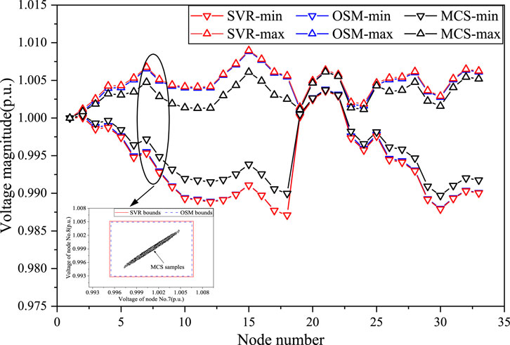
Figure 6. The voltage interval results obtained by SVR, OSM and MCS for IEEE 33bw case in Scenario 1.
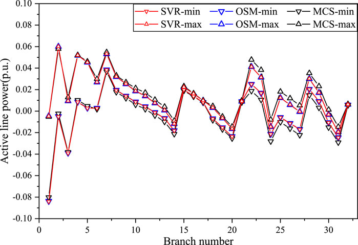
Figure 7. The active line power interval results obtained by SVR, OSM and MCS for IEEE 33bw case in Scenario 1.
5.1.2.2 The simulation under scenario 2
In Scenario 2, the original active power generation data was listed in Table 2, and the fluctuation coefficients were set as
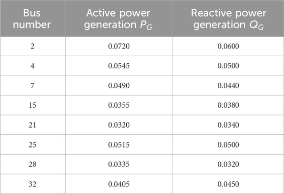
Table 2. The original power generation data of DGs for IEEE 33bw case in Scenario 2 (p.u.).
The interval bound results obtained by the SVR, OSM, and MCS for the voltage magnitudes of nodes and the active transmission power of branches for IEEE 33bw case in Scenario 2 are presented in Figures 8, 9, respectively. Similarly, the voltage interval boundaries of nodes No. 4 and No. 5 are selected in Figure 8 for comparison with the MCS sampling results. The SVR is observed to have acquired a similar voltage range to OSM, which is wider than that of MCS. The active line power interval bounds acquired by SVR are close to that obtained by OSM and MCS. These results show that the proposed method also has high precision under scenario 2, which proves that the SVR-based IPF prediction model can adapt to different operating points.
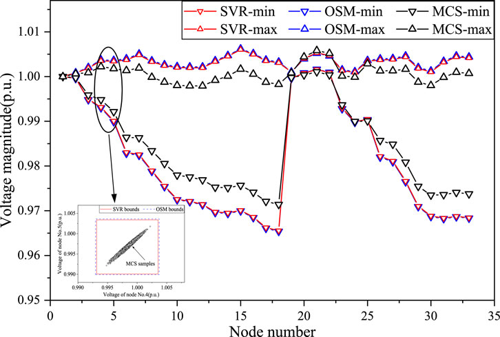
Figure 8. The voltage interval results obtained by SVR, OSM and MCS for IEEE 33bw case in Scenario 2.
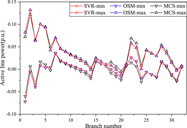
Figure 9. The active line power interval results obtained by SVR, OSM and MCS for IEEE 33bw case in Scenario 2.
5.1.2.3 The simulation under scenario 3
In Scenario 3, the original active power generation data was the same as that in Table 2, and the fluctuation coefficients were set as
Scenario 3 was set up to verify the accuracy of the proposed algorithm when the operating points and fluctuation ranges change simultaneously. The interval bounds of voltage and active line power obtained by SVR, OSM, and MCS in Scenario 3 are presented in Figures 10, 11. Besides, the voltage boundaries of nodes No. 6 and No. 7 obtained by SVR and OSM are also compared with the MCS sampling results in Figure 10. It can be observed that the voltage ranges obtained by SVR and OSM are still very close, which are more conservative than those obtained by MCS. The active line power ranges acquired by the three methods remain close. The simulation results are expected. Furthermore, compared to scenario 2, the voltage and active line power interval ranges obtained by the three methods are both smaller. This is because the fluctuation ranges are reduced while the operating points remain still. The simulation in scenario 3 validates that the proposed algorithm can maintain high prediction accuracy under different operating points and fluctuation ranges.
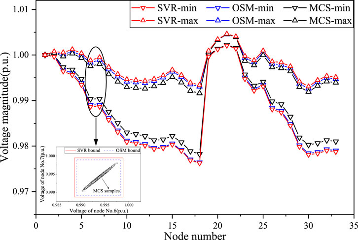
Figure 10. The voltage interval results obtained by SVR, OSM and MCS for IEEE 33bw case in Scenario 3.
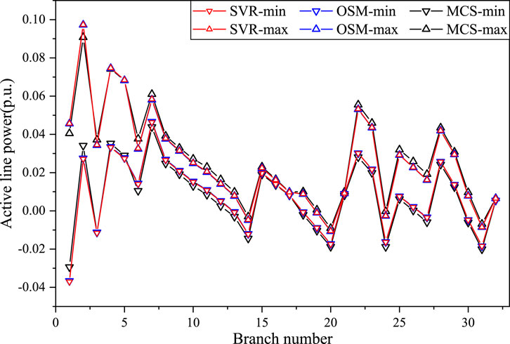
Figure 11. The active line power interval results obtained by SVR, OSM and MCS for IEEE 33bw case in Scenario 3.
In summary, based on simulations under different scenarios, the proposed SVR-based IPF prediction model can adapt to various operational states and environmental fluctuations. In different operating scenarios, this method achieves prediction accuracy comparable to the OSM which is model-driven. Besides, the SVR method provides a more conservative interval range than MCS, which ensures distribution system security under high-dimensional uncertainty. It demonstrates high computational accuracy and strong adaptability of the proposed approach.
5.2 IEEE 69 case study
The IEEE 69 case is applied to validate the efficiency of the proposed SVR-based IPF prediction method. The distribution network is enhanced to include eight DGs. The topology of enhanced IEEE 69 case is presented in Figure 12 and the original active and reactive power generation of DGs are shown in Table 3. All parameters are valued in p.u., and the base power is set to 10 MVA. The voltage limits of all nodes except the slack bus are constrained to [0.9, 1.1].
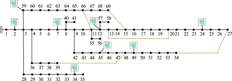
Figure 12. The topology of enhanced IEEE 69 distribution network.

Table 3. The original power generation data of DGs for IEEE 69 case (p.u.).
In IEEE 69 case, 500 sets of training data were generated under the condition of fluctuations with
To further demonstrate the advantage of the proposed SVR-based IPF method, this case additionally incorporated the Random Forest (RF) method for interval power flow prediction. To balance both prediction accuracy and efficiency, the parameters for training the RF model were set as follows: the number of decision trees was set to 100, the minimum leaf size was set to 5, and the model was configured as a regression model. Besides, the system uncertainty parameters were consistent with those described above. Considering the above all, the simulation results are presented in Figures 13, 14.
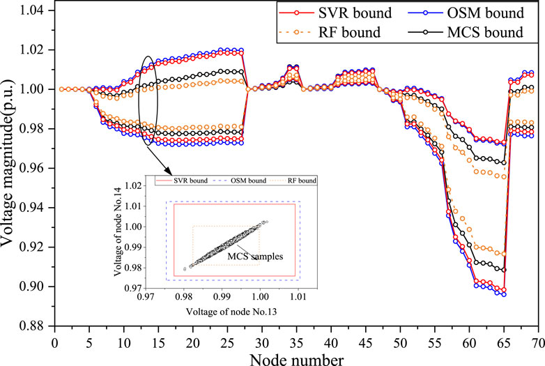
Figure 13. The voltage interval results obtained by SVR, RF, OSM and MCS for IEEE 69 case.
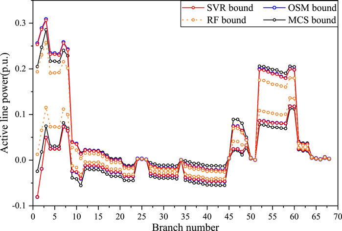
Figure 14. The active line power interval results obtained by SVR, RF, OSM and MCS for IEEE 69 case.
Figures 13, 14 show the voltage interval ranges and active line transmission power ranges, respectively. The voltage bounds of nodes No. 13 and No. 14 obtained by SVR, RF and OSM are depicted in Figure 13 compared with the MCS samples. It can be observed that under large-scale fluctuations, the voltage ranges obtained by the SVR and OSM are relatively close, and the error precision is determined to be 0.001 upon calculations. The error is mainly attributed to the insufficient size of the training dataset, which can be mitigated by increasing the number of training samples. However, the two methods yield very close active transmission power ranges with high prediction accuracy. Furthermore, compared to the MCS, SVR and OSM obtain wider voltage ranges, as explained in 5.1.2. This case study validates the adaptability of the proposed method to different networks and their ability to handle large fluctuation ranges.
Comparing the SVR method proposed in this paper with the RF method, the SVR method achieves higher prediction accuracy. It is evident that the prediction error using the RF method is relatively large, with an error precision of only 0.01, which shows a significant deviation from the interval results obtained by the OSM. Additionally, the interval obtained by the RF method is narrower, possibly because the predictions of the trees in the model are more concentrated and less flexible in handling extreme cases. Meanwhile, for the RF method, improving prediction accuracy requires increasing the number of decision trees, but this comes at the cost of increased computation time. Through multiple experiments, the accuracy gain from adding more decision trees was found to be negligible.
To validate the efficiency of the proposed method, the computation time of the algorithm compared to RF and OSM is shown in Table 4. The computation time includes the total time for solving voltage and line transmission power. It is noticeable that the online computation speed of the SVR-based IPF prediction method and RF prediction method is significantly faster than the OSM. Meanwhile, the online computation speed of SVR is also faster than that of RF. Besides, the offline training of SVR and RF requires more time compared to the OSM computation, and the offline training times of SVR and RF are comparable. However, the training and OSM both require significant amounts of time, which increases as the number of system nodes grows. In contrast, the online computation time of SVR is minimally affected by the system scale, and predictions are conducted based on the trained results in practical applications, so that the online computation time is more crucial.
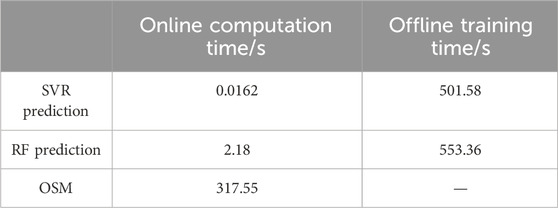
Table 4. The computation time of SVR prediction method, RF prediction method, and OSM for IEEE 69 case.
The comparison demonstrates that the proposed SVR approach achieves a significant improvement in computational efficiency over model-driven approaches and is more suitable for large-scale systems. Additionally, the SVR approach has advantages over the RF method in both computational accuracy and efficiency, demonstrating that it is more suitable for IPF analysis compared to other data-driven methods. In summary, the proposed SVR approach is more suitable for rapid and real-time PF analysis of distribution networks with DGs.
6 Conclusion
To address the uncertainty in PF and overcome the efficiency challenges faced by traditional model-driven methods, an SVR-based IPF prediction method for PF analysis in distribution networks is proposed through combining data-driven methods with interval theory. This method considers uncertainty as intervals and employs SVR for model training. The training data is generated through simulation of the established IPF model for distribution network including the intervals of node power injections, line parameters, and the minimum/maximum PF variables. Then the input and output feature vectors for IPF are constructed and the multi-output SVR-based IPF prediction model is established based on the training dataset. To assess the performance of the proposed method, several simulations are conducted both on IEEE 33bw case and IEEE 69 case.
The simulation results show that the proposed method has a good performance. Firstly, the evaluation metrics are calculated to demonstrate the method’s high accuracy. Additionally, the proposed method is compared with OSM and MCS in three different scenarios, showcasing robust adaptability across different distribution network cases, operating points, and input data fluctuation ranges. The comparison of interval results obtained by SVR prediction and OSM demonstrates that the SVR approach can achieve prediction accuracy comparable to that of model-driven methods. Meanwhile, the comparative analysis of computation time with the OSM and RF demonstrates that the proposed approach significantly improves computational efficiency compared to model-driven approaches and offers better prediction accuracy and efficiency compared to other data-driven methods. In conclusion, the proposed method exhibits superior computational efficiency and accuracy, meeting the requirements for handling power flow uncertainty and achieving real-time rapid PF analysis in distribution networks.
Data availability statement
The original contributions presented in the study are included in the article/supplementary material, further inquiries can be directed to the corresponding authors.
Author contributions
XL: Conceptualization, Methodology, Writing–original draft. HZ: Data curation, Investigation, Writing–review and editing. QL: Methodology, Validation, Writing–original draft, Writing–review and editing. ZL: Software, Writing–review and editing. HL: Investigation, Writing–original draft.
Funding
The author(s) declare that financial support was received for the research, authorship, and/or publication of this article. This work was supported by the Science and Technology Project of China Southern Power Grid (090000KK52222133/SZKJXM20222115).
Conflict of interest
Authors XL, HZ, ZL, HL were employed by Shenzhen Power Supply Co., Ltd.
The remaining author declare that the research was conducted in the absence of any commercial or financial relationships that could be construed as a potential conflict of interest.
The authors declare that this study received funding from China Southern Power Grid. The funder had the following involvement in the study: data curation, investigation, the study methodology, data analysis, and writing-review\editing.
Publisher’s note
All claims expressed in this article are solely those of the authors and do not necessarily represent those of their affiliated organizations, or those of the publisher, the editors and the reviewers. Any product that may be evaluated in this article, or claim that may be made by its manufacturer, is not guaranteed or endorsed by the publisher.
References
Barboza, L. V., Dimuro, G. P., and Reiser, R. S. (2004). “Towards interval analysis of the load uncertainty in power electric systems,” in Proceedings of the international conference on probabilistic methods applied to power systems (ICPMAPS), ames, United States, 12-16 september 2004, 538–544.
Cao, Y., Zhou, B., Chung, C. Y., Wu, T., Zheng, L., and Shuai, Z. (2024). A coordinated emergency response scheme for electricity and watershed networks considering spatio-temporal heterogeneity and volatility of rainstorm disasters. IEEE Trans. Smart Grid. 15 (4), 3528–3541. doi:10.1109/TSG.2024.3362344
Chen, J., Li, W., Wu, W., Zhu, T., Wang, Z., and Zhao, C. (2020). “Robust data-driven linearization for distribution three-phase power flow,” in Proceedings of the IEEE 4th conference on energy internet and energy system integration (EI2), 1527–1532. Wuhan, China, 30 October-01 November 2020.
Chen, J., Wu, W., and Roald, L. A. (2022). Data-driven piecewise linearization for distribution three-phase stochastic power flow. IEEE Trans. Smart Grid. 13 (2), 1035–1048. doi:10.1109/TSG.2021.3137863
Chen, Y., Wu, C., and Qi, J. (2022). Data-driven power flow method based on exact linear regression equations. J. Mod. Power Syst. Clean. Energy. 10 (3), 800–804. doi:10.35833/MPCE.2020.000738
Cheng, S., Zuo, X., Yang, K., Wei, Z., and Wang, R. (2023). Improved affine arithmetic-based power flow computation for distribution systems considering uncertainties. IEEE Syst. J. 17 (2), 1918–1927. doi:10.1109/JSYST.2022.3176461
Dong, M., Wiebe, D., and Shi, J. (2022). “An accelerated and risk-free AC power flow method with machine learning based initiation,” in Proceedings of the IEEE electrical power and energy conference (EPEC), 103–108. Victoria, Canada, 05-07 December 2022.
Fu, X., Zhang, C., Xu, Y., Zhang, Y., and Sun, H. (2024). Statistical machine learning for power flow analysis considering the influence of weather factors on photovoltaic power generation. IEEE Trans. Neural Netw. Learn. Syst., 1–15. doi:10.1109/TNNLS.2024.3382763
Guo, L., Zhang, Y., Li, X., Wang, Z., Liu, Y., Bai, L., et al. (2022). Data-driven power flow calculation method: a lifting dimension linear regression approach. IEEE Trans. Power Syst. 37 (3), 1798–1808. doi:10.1109/TPWRS.2021.3112461
Hu, X., Hu, H., Verma, S., and Zhang, Z. L. (2021). Physics-guided deep neural networks for power flow analysis. IEEE Trans. Power Syst. 36 (3), 2082–2092. doi:10.1109/TPWRS.2020.3029557
Jia, M., and Hug, G. (2023). “Overview of data-driven power flow linearization,” in Proceedings of the IEEE belgrade PowerTech, 1–6. Belgrade, Serbia, 25-29 June 2023.
Khalid, H. M., Muyeen, S. M., and Kamwa, I. (2022). An improved decentralized finite-time approach for excitation control of multi-area power systems. Sustain. Energy Grids Netw. 31 31, 100692. doi:10.1016/j.segan.2022.100692
Leng, S., Liu, K., Ran, X., Chen, S., and Zhang, X. (2020). An affine arithmetic-based model of interval power flow with the correlated uncertainties in distribution system. IEEE Access 8, 60293–60304. doi:10.1109/ACCESS.2020.2982928
Li, P., Wu, W., Wang, X., and Xu, B. (2023). A data-driven linear optimal power flow model for distribution networks. IEEE Trans. Power Syst. 38 (1), 956–959. doi:10.1109/TPWRS.2022.3216161
Liang, Z., Dong, Z., Li, C., Wu, C., and Chen, H. (2023). A data-driven convex model for hybrid microgrid operation with bidirectional converters. IEEE Trans. Smart Grid. 14 (2), 1313–1316. doi:10.1109/TSG.2022.3193030
Liu, J., Yang, Z., Zhao, J., Yu, J., Tan, B., and Li, W. (2022). Explicit data-driven small-signal stability constrained optimal power flow. IEEE Trans. Power Syst. 37 (5), 3726–3737. doi:10.1109/TPWRS.2021.3135657
Liu, Y., Li, Z., and Zhao, J. (2022). Robust data-driven linear power flow model with probability constrained worst-case errors. IEEE Trans. Power Syst. 37 (5), 4113–4116. doi:10.1109/TPWRS.2022.3189543
Liu, Y., Li, Z., and Zhou, Y. (2022). Data-driven-aided linear three-phase power flow model for distribution power systems. IEEE Trans. Power Syst. 37 (4), 2783–2795. doi:10.1109/TPWRS.2021.3130301
Liu, Y., Wang, Y., Zhang, N., Lu, D., and Kang, C. (2020). A data-driven approach to linearize power flow equations considering measurement noise. IEEE Trans. Smart Grid. 11 (3), 2576–2587. doi:10.1109/TSG.2019.2957799
Liu, Y., Xu, B., Botterud, A., Zhang, N., and Kang, C. (2021). Bounding regression errors in data-driven power grid steady-state models. IEEE Trans. Power Syst. 36 (2), 1023–1033. doi:10.1109/TPWRS.2020.3017684
Lyu, C., Sheng, W., Liu, K., and Dong, X. (2023). Novel affine power flow method for improving accuracy of interval power flow data in cyber physical systems of active distribution networks. CSEE J. Power Energy Syst. 9 (5), 1881–1892. doi:10.17775/CSEEJPES.2020.07040
Mezghani, I., Misra, S., and Deka, D. (2020). Stochastic AC optimal power flow: a data-driven approach. Electr. Power Syst. Res. 189, 106567. doi:10.1016/j.epsr.2020.106567
Mori, H., and Yuihara, A. (1999). “Calculation of multiple power flow solutions with the Krawczyk method,” in Proceedings of the IEEE international symposium on circuits and systems (ISCAS), 94–97. Orlando, USA.
Musleh, A. S., Khalid, H. M., Muyeen, S. M., and Al-Durra, A. (2019). A prediction algorithm to enhance grid resilience toward cyber attacks in WAMCS applications. IEEE Syst. J. 13 (1), 710–719. doi:10.1109/JSYST.2017.2741483
Rehman, A. U., Ullah, Z., Qazi, H. S., Hasanien, H. M., and Khalid, H. M. (2024). Reinforcement learning-driven proximal policy optimization-based voltage control for PV and WT integrated power system. Renew. Energy. 227, 120590. doi:10.1016/j.renene.2024.120590
Shao, Z., Zhai, Q., and Guan, X. (2023). Physical-model-aided data-driven linear power flow model: an approach to address missing training data. IEEE Trans. Power Syst. 38 (3), 2970–2973. doi:10.1109/TPWRS.2023.3256120
Sun, Y., Zhao, Z., Yang, M., Jia, D., Pei, W., and Xu, B. (2020). Overview of energy storage in renewable energy power fluctuation mitigation. CSEE J. Power Energy Syst. 6 (1), 160–173. doi:10.17775/CSEEJPES.2019.01950
Tan, B., Chen, S., Liang, Z., Zheng, X., Zhu, Y., and Chen, H. (2024). An iteration-free hierarchical method for the energy management of multiple-microgrid systems with renewable energy sources and electric vehicles. Appl. Energy. 356, 122380. doi:10.1016/j.apenergy.2023.122380
Tan, Y., Chen, Y., Li, Y., and Cao, Y. (2020). Linearizing power flow model: a hybrid physical model-driven and data-driven approach. IEEE Trans. Power Syst. 35 (3), 2475–2478. doi:10.1109/TPWRS.2020.2975455
Vaccaro, A., Canizares, C. A., and Villacci, D. (2010). An affine arithmetic-based methodology for reliable power flow analysis in the presence of data uncertainty. IEEE Trans. Power Syst. 25 (2), 624–632. doi:10.1109/TPWRS.2009.2032774
Xing, Z., Gong, J., Lao, K. W., and Dai, N. (2021). “Single bus data-driven power estimation based on modified linear power flow model,” in Proceedings of the 6th international conference on power and renewable energy (ICPRE) (Shanghai, China), 755–758.
Xing, Z., Lao, K. W., Gao, H., and Dai, N. (2022). “A modified data-driven power flow model for power estimation with incomplete bus data,” in Proceedings of the 12th international conference on power, energy and electrical engineering (CPEEE), 316–320. Shiga, Japan, 25-27 February 2022.
Xue, Y., and Liu, Y. (2021). Intelligent assessment of active and reactive power flow with satisfying accuracy for N-k1-k2 cascading outages. J. Mod. Power Syst. Clean. Energy. 9 (5), 986–999. doi:10.35833/MPCE.2020.000312
Zhang, C., Chen, H., Ngan, H., Yang, P., and Hua, D. (2017). A mixed interval power flow analysis under rectangular and polar coordinate system. IEEE Trans. Power Syst. 32 (2), 1–1429. doi:10.1109/TPWRS.2016.2583503
Zhang, C., Chen, H., Shi, K., Qiu, M., Hua, D., and Ngan, H. (2018). An interval power flow analysis through optimizing-scenarios method. IEEE Trans. Smart Grid. 9 (5), 5217–5226. doi:10.1109/TSG.2017.2684238
Zhang, C., Liu, Q., Zhou, B., Chung, C. Y., Li, J., Zhu, L., et al. (2023). A central limit theorem-based method for DC and AC power flow analysis under interval uncertainty of renewable power generation. IEEE Trans. Sustain. Energy. 14 (1), 563–575. doi:10.1109/TSTE.2022.3220567
Keywords: data-driven method, interval power flow, support vector regression, distribution network, distributed generators
Citation: Liang X, Zhang H, Liu Q, Liu Z and Liu H (2024) A support vector regression-based interval power flow prediction method for distribution networks with DGs integration. Front. Energy Res. 12:1465604. doi: 10.3389/fenrg.2024.1465604
Received: 16 July 2024; Accepted: 17 September 2024;
Published: 30 September 2024.
Edited by:
Ying Zhang, Oklahoma State University, United StatesReviewed by:
Zipeng Liang, Hong Kong Polytechnic University, Hong Kong SAR, ChinaHaoyong Chen, South China University of Technology, China
Yun Liu, South China University of Technology, China
Ge Chen, Purdue University, United States
Haris M. Khalid, University of Dubai, United Arab Emirates
Copyright © 2024 Liang, Zhang, Liu, Liu and Liu. This is an open-access article distributed under the terms of the Creative Commons Attribution License (CC BY). The use, distribution or reproduction in other forums is permitted, provided the original author(s) and the copyright owner(s) are credited and that the original publication in this journal is cited, in accordance with accepted academic practice. No use, distribution or reproduction is permitted which does not comply with these terms.
*Correspondence: Huaying Zhang, emh5dGd5eEAxNjMuY29t; Qian Liu, bGl1cWlhbjM2NUBobnUuZWR1LmNu