Safe dynamic optimization of automatic generation control via imitation-based reinforcement learning

Introduction: The increasing penetration of distributed generation (e.g., solar power and wind power) in the energy market has caused unpredictable disturbances in power systems and accelerated the application of intelligent control, such as reinforcement learning (RL), in automatic generation control (AGC). However, traditional RL cannot ensure constraint safety during training and frequently violates the constraints (e.g., frequency limitations), further threatening the safety and stability of grid operation.

Methods: To address the safety issue, we propose a novel safe RL framework that combines expert experiences with the RL controller to achieve imitation-based RL. This method allows an initialized safe policy by imitating expert experiences to prevent random explorations at the beginning. Specifically, we first formulate the AGC problem mathematically as a Markov decision process. Then, the imitation mechanism is developed atop a soft actor–critic RL algorithm.

Results and discussion: Finally, numerical studies are conducted with an IEEE 39-bus network, which show that the proposed method satisfies the frequency control performance standard better and improves the RL training efficiency.

1 Introduction

Automatic generation control (AGC) is a fundamental part of a power system that is important for realizing system frequency stability and smoothing tie-line power among interconnected grids (Yu et al., 2024b). Regional power grid dispatch centers are often required to achieve closed-loop correction control on area control errors (ACEs) based on real-time deviations (Peddakapu et al., 2022). Generally, these ACEs are influenced by large fluctuations and uncertain photovoltaic outputs that decrease the power quality significantly (Kumar et al., 2023a; Satapathy and Kumar, 2020). Many researchers have focused on different methods to handle these quality problems, such as AGC and demand-side resources (Kumar et al., 2023b; Kumar, 2024). The control performance standard (CPS) for assessing AGC strategies was established in 1999 by the North American Electric Reliability Council (NERC) (Jaleeli and VanSlyck, 1999) and focuses on the medium- and long-term stability performances of the system frequency as well as tie-line power. Therefore, an efficient AGC strategy is of great significance in improving the CPS and realizing the economical distribution of grids.

Generally, the time scale for AGC strategies is rather short and of the order of 2–8 s. These AGC strategies entail two control processes: (1) determination of the total power adjustment according to the observed system operating state; (2) allocation of this determined total power adjustment among the AGC units to correct the ACEs and minimize energy costs. At present, research on conventional AGC strategies has achieved fruitful results, such as proportional integral derivative (PID) control (Dahiya et al., 2016; Sahu et al., 2015), model predictive control (Oshnoei et al., 2020), and learning-based intelligent control (Xi et al., 2020). However, conventional AGC has a typical feedback delay that may lead to overregulation or underregulation when coordinating different AGC units (e.g., water and thermal power units). In addition, given the increasing penetration of wind generation, centralized grid connections of wind power can cause large amounts of minute-level power fluctuations (Wang et al., 2023). This further complicates AGC-based regulation and places a greater burden on real-time coordinated AGC. To cope with the increasing power fluctuations and hysteresis issues, the concept of dynamic optimization of AGC has been proposed (Yan et al., 2013), whose key idea is optimization of the AGC units in advance based on ultrashort-term forecasting of the future loads and renewables (e.g., wind power). Unlike economic dispatch (for the next 15 min) and conventional AGC (response within 2–8 s), dynamically optimized AGC is considered a middle process for optimizing the AGC units within 15 min at an optimization step of 1 min. The main advantage of AGC dynamic optimization is that it can effectively handle short-term fluctuations (within 15 min) caused by renewables because it takes into account the future load and renewables. Therefore, AGC dynamic optimization has significant impacts on power systems with stochastic renewables.

Generally, optimization programming is adopted as the most common approach to solve the AGC dynamic control problem using the probabilistic model of wind power, such as robust optimization (Zhang et al., 2024). For instance, Zhao et al. (2019) proposed a chance-constrained programming method to solve the dynamic dispatch of AGC units by combining the evolutionary programming algorithm with the point estimation method to solve the stochastic wind power model. Zhang et al. (2015) developed an improved multiobjective optimization model of AGC dispatch using the genetic algorithm to solve for the dispatch model; this work established an accurate dispatch model based on real-time data of the phasor measurement units. Zhang et al. (2020) used the model predictive control framework to effectively address real-time dispatch given the dynamic variations of AGC signals between adjacent dispatch intervals. Wang et al. (2018) used robust optimization to address uncertain wind power information by converting it into boundary information of the prediction interval; then, a decentralized robust optimization method was proposed based on approximate dynamic programming to solve for the robust AGC dispatch model. However, all of the above works rely heavily on the accurate probability model of renewables, which is difficult to obtain in practice. Moreover, stochastic programming is usually non-convex owing to the uncertainty involved and is difficult to solve as it entails a large computational burden. Hence, the future fluctuations of renewables cannot be effectively considered in the AGC dispatch process.

Through the adoption of neural networks for uncertainty predictions (Wang and Zhang, 2024), deep reinforcement learning (RL) has become increasingly popular for handling the AGC dynamic optimization problem as it is robust with stable convergence results (Cheng and Yu, 2019; Ruan et al., 2024). For instance, Li et al. (2021) proposed a multiple-experience pool-replay-twin-delayed deep deterministic policy gradient to solve for AGC dispatch that effectively improved the training efficiency and action quality via four improvements, including the multiple-experience pool probability replay strategy. Zheng et al. (2021) designed a linear active disturbance rejection control scheme based on the tie-line bias control mode and solved the control problem using the soft actor–critic (SAC) RL algorithm. Liu et al. (2022) adopted the proximal policy optimization RL algorithm to optimize power regulation among the AGC units in advance so as to ensure that the frequency characteristics could better satisfy the CPS under large fluctuations in power systems. However, given that online training interacts with real-world systems, any RL strategy must be trained through trial-and-error extensively before being considered intelligent (Wang et al., 2022). This means that some “bad” decisions may be made during training, some of which may cause critical frequency violations. This is unsafe and unacceptable for real-world AGC problems. Therefore, direct application of traditional RL methods is not ideal for coping with such critical constraints because the strategy involves learning with frequent constraint violations.

To address the limitations of conventional RL algorithms, we propose a safe RL framework to ensure that the critical constraints are satisfied during training. Generally, trial-and-error conditions occur during the initial stages of training because the initialized policy is random and not satisfactory (Yu et al., 2024a; Yang et al., 2024). Hence, to avoid early random explorations in RL, we adopt imitation learning to train an initialized policy that is similar to expert experiences; this training is performed offline without interactions with real-world grids. Then, based on the imitated policy as the initialization, the SAC RL algorithm is used to further train an optimal AGC strategy online (Haarnoja et al., 2018). The main contributions of this work are as follows: (1) the AGC dynamic optimization problem is formulated as a Markov decision process (MDP) to consider both the dispatch economy and CPS; (2) imitation learning based on expert experiences is designed on top of the traditional RL framework to prevent significant frequency violations during training; (3) the state-of-the-art SAC algorithm is adopted as it is model-free and can effectively cope with uncertainties from the short-term fluctuations of renewables.

The remainder of this manuscript is organized as follows. Section 2 introduces the AGC problem and its mathematical formulation as an MDP. Section 3 presents the imitation-based safe RL framework for solving the proposed MDP. Section 4 outlines the numerical studies conducted based on the proposed approach. Section 5 presents the conclusions of this study.

2 Problem statement and MDP formulation for AGC

2.1 System model and AGC problem statement

Figure 1 shows the conventional AGC dynamic optimization scheme for optimizing the regulated power of AGC units in steps of 1 min over a duration of 15 min based on the deviation information for system frequency, ACE, and tie-line power. Generation units in a power grid are of two types, namely AGC and non-AGC units, whose power outputs are denoted as $P_i^{\text{AG}}$ and $P_g^{\text{NG}}$, respectively. Here, $i$ and $g$ are both the indices of the AGC and non-AGC units. In this work, the AGC units participate in both primary and secondary frequency control, while the non-AGC units only provide primary frequency control. Hence, the dynamic power outputs can be calculated as follows:

$\begin{array}{ll}\hfill & P_{g,t+1}^{\text{NG}}=P_{g,t}^{\text{NG}}-K_g\left(\mathrm{\Delta }{f}_{t+1}-\mathrm{\Delta }{f}_t\right),\hfill \end{array}(1)$

$\begin{array}{ll}\hfill & P_{i,t+1}^{\text{AG}}=P_{i,t}^{\text{AG}}-K_i\left(\mathrm{\Delta }{f}_{t+1}-\mathrm{\Delta }{f}_t\right)+\mathrm{\Delta }{P}_{i,t}^{\text{AGC}},\hfill \end{array}(2)$

where $\mathrm{\Delta }{f}_{t+1}$ and $\mathrm{\Delta }{f}_t$ are the frequency deviations at time $t+1$ and $t$, respectively; $\mathrm{\Delta }{P}_{i,t}^{\text{AGC}}$ is the power adjustment of the AGC unit $i$ at time $t$ for secondary frequency control; $K_i$ and $K_g$ are the frequency regulation constants of the AGC unit $i$ and non-AGC unit $g$, respectively. Here, Equation 2 includes two parts, which are the primary frequency control power $K_i(\mathrm{\Delta }{f}_{t+1}-\mathrm{\Delta }{f}_t)$ of the AGC unit $i$ and power increment of the AGC unit $\mathrm{\Delta }{P}_{i,t}^{\text{AGC}}$ at each optimization time. Thus, the AGC units respond to the uncertain power fluctuations in the grid through power regulation $\mathrm{\Delta }{P}_{i,t}^{\text{AGC}}$ at time $t$.

Figure 1

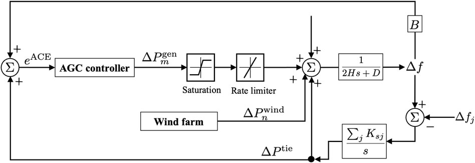
Figure 1. Diagram of area frequency coordination control.

From Figure 1, we see that the AGC strategy requires three dynamic system parameters as inputs: frequency $\mathrm{\Delta }{f}_t$, ACE $e_t^{\text{ACE}}$, and tie-line power $P_t^{\text{tie}}$. Hence, their system dynamics are as follows:

$\frac{d(\mathrm{\Delta }{f}_t)}{dt}=-\frac{D}{2H}\mathrm{\Delta }{f}_t+\frac{1}{2H}(\mathrm{\Delta }{P}_t^{\text{wind}}+\mathrm{\Delta }{P}_t^{\text{tie}}+\mathrm{\Delta }{P}_t^{\text{gen}}+\mathrm{\Delta }{P}_t^{\text{d}})(3)$

$\begin{array}{ll}\hfill & e_t^{\text{ACE}}=\mathrm{\Delta }{P}_t^{\text{tie}}+10B\cdot \mathrm{\Delta }{f}_t,\hfill \end{array}(4)$

$\begin{array}{ll}\hfill & \frac{d\left(\mathrm{\Delta }{P}_t^{\text{tie}}\right)}{dt}={\sum }_j{K}_{sj}\cdot \left(\mathrm{\Delta }{f}_t-\mathrm{\Delta }{f}_{j,t}\right),\hfill \end{array}(5)$

where $H$ is the equivalent inertial constant; $D$ is the equivalent damping coefficient; $\mathrm{\Delta }{P}_t^{\text{wind}}$, $\mathrm{\Delta }{P}_t^{\text{gen}}$ and $\mathrm{\Delta }{P}_t^{\text{d}}$ are power adjustments of wind, generation, and demands at time t; $B$ is the frequency regulation constant of the control system in megawatts per 0.1 Hz (positive value); $K_{sj}$ and $\mathrm{\Delta }{f}_{j,t}$ are the tie-line synchronization coefficient and frequency deviation of the connected $j$-region, respectively; $P_t^{\text{tie}}$ is the tie-line power outflow that is considered to be positive; $\mathrm{\Delta }{P}_t^{\text{tie}}$ is the tie-line power deviation. Equations 1–5 describe the system dynamics of key variables.

In the present work, our control objective is to schedule the AGC units so as to satisfy both the minimum economic cost of auxiliary services as well as stability and safety of the CPS. Therefore, the objective can be expressed mathematically as follows:

$\min f_1={\displaystyle \sum _{i\in \text{ACG\hspace{0.17em}units}}}{c}_i\left(|P_{i,t}^{\text{AG}}-P_{i,0}^{\text{AG}}|+u_{i,t}{R}_{i,t}^{\text{AG}}\right),(6)$

where $c_i$ is the auxiliary service cost coefficient of the AGC unit $i$; $R_{i,t}^{\text{AG}}$ is the climbing power at time $t$ of the AGC unit $i$; $u_{i,t}\in -\mathrm{1,0,1}$ indicates the change in the direction of the power output, where $u_{i,t}=-1$ denotes a decrease, $u_{i,t}=1$ denotes an increase, and $u_{i,t}=0$ denotes that there is no change.

The assessment indexes of the CPS include CPS1 and CPS2. Here, CPS1 is defined to evaluate the correlation between the system frequency deviation and ACE, while CPS2 is defined as the average ACE over 15 min, indicating that the ACE is maintained within a tolerance range to ensure that the power exchanged between the regions does not exceed the specified limits. The detailed definitions of CPS1 and CPS2 are as follows:

$\begin{array}{ll}\hfill & K^{\text{cps}1}=\frac{{\sum }_{t=1}^T{e}_t^{\text{ACE}}}{|T|}\cdot \frac{{\sum }_{t=1}^T\left(f_t-f^{\text{ref}}\right)}{|T|}\cdot \frac{1}{10B{ϵ}_1^2},\hfill \end{array}(7)$

$\begin{array}{ll}\hfill & K^{\text{cps}2}=|\frac{1}{|T|}{\sum }_{t=1}^T\left(\mathrm{\Delta }{P}_t^{\text{tie}}+10B\cdot \mathrm{\Delta }{f}_t\right)|,\hfill \end{array}(8)$

where $T$ is the time interval; $f^{\text{ref}}$ is the rated frequency; ${ϵ}_1$ represents the frequency control target, which is usually taken as the root mean-squared (RMS) value of the mean frequency deviation of 1 min in the previous year. In practice, when CPS1 satisfies the condition $K^{\text{cps}1}\ge 2$, CPS2 will not be assessed (Wu et al., 2010); otherwise, CPS2 must be less than the following threshold:

$K^{\text{cps}2}\le 1.65{ϵ}_{15min}\sqrt{100B{B}_s},(9)$

where ${ϵ}_{15min}$ is the RMS value of the mean frequency deviation over 15 min in the previous year; $B_s$ is the equivalent frequency regulation constant for the entire interconnection power grid. If CPS1 is suitably satisfied in this work, CPS2 will not be considered an objective or a hard constraint.

The operational constraints for AGC dynamic optimization include system power balance, AGC unit regulation characteristics, and limits for the frequency and tie-line power deviations. The basic power balance constraint must satisfy the condition

${\displaystyle \sum _i}{P}_{i,t}^{\text{AG}}+{\displaystyle \sum _g}{P}_{g,t}^{\text{NG}}+P_t^{\text{wind}}-P_t^{\text{D}}-P_t^{\text{tie}}-P_t^{\text{loss}}=0,(10)$

where $P_t^{\text{wind}}$ and $P_t^{\text{D}}$ are the forecast values of the wind power and loads for period $t$; $P_t^{\text{loss}}$ is the line transmission loss.

As shown in Figure 1, the saturation function and ramp rate limiter will take effect on the control signals before being executed. Specifically, the power output and ramp power constraints of AGC units are defined as follows:

$\begin{array}{ll}\hfill & {\underline{P}}_i^{\text{AG}}\le P_{i,t}^{\text{AG}}\le {\bar{P}}_i^{\text{AG}},\hfill \end{array}(11)$

$\begin{array}{ll}\hfill & {\underline{R}}_i^{\text{AG}}\le R_{i,t}^{\text{AG}}\le {\bar{R}}_i^{\text{AG}},\hfill \end{array}(12)$

where ${\bar{P}}_i^{\text{AG}}$ and ${\underline{P}}_i^{\text{AG}}$ are the upper and lower limits of the output power of the $i$-th AGC unit, respectively; ${\bar{R}}_i^{\text{AG}}$ and ${\underline{R}}_i^{\text{AG}}$ are the upper and lower limits of the ramp power of the $i$-th AGC unit, respectively. Moreover, the limitations on the frequency deviation and tie-line power are as follows:

$\begin{array}{ll}\hfill & \mathrm{\Delta }\underline{f}\le \mathrm{\Delta }{f}_t\le \mathrm{\Delta }\bar{f},\hfill \end{array}(13)$

$\begin{array}{ll}\hfill & {\underline{P}}^{\text{tie}}\le P_t^{\text{tie}}\le {\bar{P}}^{\text{tie}},\hfill \end{array}(14)$

where $\mathrm{\Delta }\bar{f}$ and $\mathrm{\Delta }\underline{f}$ are the corresponding upper and lower limits of the system frequency deviation, respectively; ${\bar{P}}^{\text{tie}}$ and ${\underline{R}}^{\text{tie}}$ are upper and lower limits of the tie-line power, respectively.

2.2 MDP formulation

In this work, the MDP is a mathematical framework used to model the AGC dynamic optimization problem as a sequential decision-making process, as shown in Figure 2. The MDP is defined by a tuple $⟨\mathcal{S,A,P,R},\gamma ⟩$, where $\mathcal{S}$ is a set of states, $\mathcal{A}$ is a set of actions, $\mathcal{P}$ is a transition model that gives the probability of moving from one state to another when given an action, $\mathcal{R}$ is a reward function that provides the immediate reward for state transitions, and $\gamma \in [\mathrm{0,1}]$ is a discount factor that determines the importance of future rewards¹. In the MDP, the AGC strategy is considered an agent that observes the grid operating state $s_t\in \mathcal{S}$ and outputs an action $a_t\in \mathcal{A}$ at each time step $t$. Then, the agent will receive an immediate reward $r_t\in \mathcal{R}$. The sequential continuous experience $\tau$ is then recorded as $\left\{{\mathit{s}}_0,{\mathit{a}}_0,{\mathit{s}}_1,\dots ,{\mathit{a}}_{T-1},{\mathit{s}}_T\right\}$. The objective of the agent is to maximize its cumulative reward $J_{\pi }$ by iteratively updating its policy $\pi$: $\mathcal{S}\to \mathcal{A}$, which is given by

${\max }_{\pi }{J}_{\pi }=\underset{\tau \sim \pi }{\mathbb{E}}\left[{\sum }_{t=0}^T{\gamma }^t{r}_t\right].(15)$

Figure 2

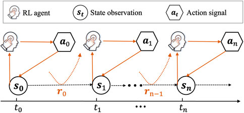
Figure 2. Interactions in the MDP.

Based on the objectives and constraints defined in Equations 6–14, we further present a well-designed MDP formulation. In this work, the control variables are the regulation direction and regulation power of each AGC unit. To simplify the action space scale using smaller action dimensions, the action is defined as the power adjustment of the AGC unit:

$a_t={\left[\mathrm{\Delta }{P}_{i,t}^{\text{AG}}|i\in I\right]}^{⊺},(16)$

where $I$ denotes the set of AGC units. Before execution, all actions are subjected to the saturation and ramp limits shown in Figure 1.

The design of the state space must capture necessary information based on two aspects: (1) conditions of the current operating system; (2) uncertain environments that must be forecast. For the former, we take into account four factors, including the current power outputs of the AGC units $P_{i,t}^{\text{AG}}$, frequency deviation $\mathrm{\Delta }{f}_t$, tie-line power deviation $\mathrm{\Delta }{P}_t^{\text{tie}}$, and ACE value $e_t^{\text{ACE}}$. For uncertain environments, we only consider wind power forecasting in this work because the load fluctuations within 15 min are usually negligible. Hence, we introduce historical wind power information to the state space for better forecasting. The system state is defined as

$s_t={\left[P_{i,t}^{\text{AG}}|i\in I,\mathrm{\Delta }{f}_t,\mathrm{\Delta }{P}_t^{\text{tie}},e_t^{\text{ACE}},\mathrm{\Delta }{P}_{t-k}^{\text{wind}}|k=\mathrm{1,2},\dots ,l,\right]}^{⊺},(17)$

where $l$ is the period of historical observations; $\mathrm{\Delta }{P}_t^{\text{wind}}=P_t^{\text{wind}}-P_{t-1}^{\text{wind}}$ denotes the difference between successive wind power outputs.

The reward design for the MDP should consider both objectives and constraints. Here, we design the reward function based on three aspects as follows:

$r_t=w_1{f}_1+w_2{\left(|K^{\text{cps}1}-2|\right)}^2+w_3{r}^{\text{penalty}},(18)$

where $w_1$, $w_2$, and $w_3$ are weight factors that balance the tradeoffs between the three subreward items; $f_1$ is the economy objective defined in Equation 6. Note that the presence of too many items will complicate the design of the corresponding weights and lead to convergence failure. Hence, we design the third item $r^{\text{penalty}}$ as a penalty for the total violations of the upper/lower limitations, such as those of the output power, ramp power, tie-line power, and frequency in Equations 11–14. The penalty term is formulated as

$r^{\text{penalty}}={\sum }_{|k|}\text{ReLU}\left(c_k-{\bar{c}}_k\right),(19)$

where $k$ represents the index of the constraints defined in Equations 11–14, i.e., $|k|=2|I|+2$; $\text{ReLU}(x)=\max (0,x)$ is a linear rectification function for measuring the violations; $c_k$ and ${\bar{c}}_k$ represent the actual index value and required limit value, respectively. Taking the constraint in Equation 13 as an example, $c_k$ and ${\bar{c}}_k$ can be defined as $c_k=\{\mathrm{\Delta }{f}_t,-\mathrm{\Delta }{f}_t\}$ and ${\bar{c}}_k=\{\mathrm{\Delta }\bar{f},-\mathrm{\Delta }\underline{f}\}$, respectively; here, we separate the original Equation 13 into two inequalities as $\mathrm{\Delta }{f}_t\le \mathrm{\Delta }\bar{f}$ and $-\mathrm{\Delta }{f}_t\le -\mathrm{\Delta }\underline{f}$, which are expressed using the same structure. Hence, Equations 16–19 show our design of four key fators in MDP formulations.

3 Imitation-based SAC for solving the MDP formulation

Figure 3 depicts the framework for the proposed imitation-based RL, which introduces imitation learning to the conventional RL scheme to improve the initialized random policy. We introduce the behavioral-cloning-based imitation learning and SAC RL algorithm separately in the following subsections.

Figure 3

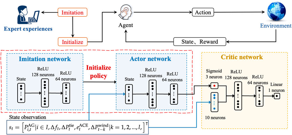
Figure 3. Proposed imitation-based RL framework.

3.1 Imitation learning based on behavioral cloning

Behavioral cloning (BC) is a common method for implementing imitation learning (Daftry et al., 2017), where the demonstrator (i.e., expert experiences) can be imitated directly without interacting with a real-world environment. The key idea of BC is to replicate the expert policy using a classifier or regressor based on previously collected training data from the encountered states and demonstrator actions (Rajaraman et al., 2020). Therefore, BC-based imitation learning can be used in an MDP framework without defining a reward function. The learning objective for the agent here is to obtain an imitation policy as the initial policy, i.e., ${\pi }_0:\mathcal{S}\to \mathcal{A}$, which is necessary to behave like an expert. Here, we adopt the variable $\xi =\{(s_0,a_0),(s_1,a_1),\dots ,(s_T,a_T)\}$ to represent the expert demonstrations.

Given the precollected set of state–action pairs $(s_i,a_i)$, the objective of the agent is to seek an imitation policy ${\pi }_0(\varphi )$ that best matches the provided set of state–action pairs. The policy network parameter $\varphi$ is then updated using maximum-likelihood estimation, i.e., the optimal ${\varphi }^{*}$ is defined as

${\varphi }^{*}=\arg {\max }_{\varphi }{\mathrm{\Pi }}_{t=0}^T{\pi }_{\varphi }\left(a_i|s_i\right).(20)$

Considering that the designed action space is continuous, we assume that the policy follows a Gaussian distribution over each action dimension. In this work, we adopt a neural network to approximate the policy $\pi$ and use the same network structure as that of the actor in the RL framework. Then, the Adam stochastic gradient descent optimizer is adopted to solve for ${\varphi }^{*}$ in Equation 20, where the gradient descent approach aims to find changes in $\varphi$ that can increase the accuracy of each imitated demonstrator action $a_i$ based on the imitation policy ${\pi }_{\varphi }(\cdot |s_i)$. The pseudocode for this process is summarized in Algorithm 1.

Algorithm 1.Behavioral-cloning-based imitation learning.

1: Initialize ${\pi }_{\varphi }$ as a random policy network

2: Define the loss function and Adam optimizer

3: Collect expert demonstration data $\xi =\{(s_i,a_i)\}$

4: Preprocess the data $\xi$ and split them into training and validation sets

5: for each policy imitation epoch do

6:  for each batch in the training data do

7:   Get the batch state–action pairs $\{(s_i,a_i)\}$

8:   Forward pass the process $a_i={\pi }_{\varphi }(s_i)$

9:   Compute loss, backward pass, and optimize the parameter $\varphi$

10:  end for

11:  Validate the policy ${\pi }_{\varphi }$ on the validation dataset

12:  Output the validation loss for the current epoch

13: end for

14: Test on the test dataset and output the test results

3.2 SAC algorithm

To solve the optimal policy ${\pi }^{*}$ in Equation 15, we adopt the SAC algorithm in this work to maximize the agent’s cumulative rewards while satisfying the safety constraints. Compared with the conventional RL algorithm, SAC uses a stochastic policy that inherently encourages exploration by adding entropy to the reward. Hence, SAC is less likely to be stuck in local optima and can better explore the action space. Moreover, incorporating policy learning with entropy regularization helps the agent to become more stable during training. The entropy term prevents the policy from becoming too deterministic too early, thereby providing a more balanced and robust learning process. The SAC objective is given as

$J_{\pi }={\sum }_{t=0}^T{\mathbb{E}}_{\tau \sim \pi }\left[r_t+\alpha \mathcal{H}\left(\pi \left(\cdot |s_t\right)\right)\right],(21)$

where $\alpha$ is the hyperparameter that balances the importance of the entropy term $\mathcal{H(·)}$ with the reward $r_t$. The entropy is calculated as follows:

$\mathcal{H}\left(\pi \left(\cdot |s_t\right)\right)=-{\mathbb{E}}_{a_t\sim \pi }\log \pi \left(a_t|s_t\right)=-\log \pi \left(\cdot |s_t\right).(22)$

For a given policy $\pi$, the state–action value function $Q:\mathcal{S}\times \mathcal{A}\to \mathbb{R}$ is defined to evaluate the expected values of the pair $(s_t,a_t)$ at time step $t$ to guide policy learning and optimization. Generally, a larger $Q$ value indicates better policy control performance. The $Q$ function is defined using the Bellman equation as follows:

$Q\left(s_t,a_t\right)\triangleq r\left(s_t,a_t\right)+\gamma {\mathbb{E}}_{s_{t+1}\sim \rho ,a_t\sim \pi }\left[Q\left(s_t,a_t\right)-\log \pi \left(a_t|s_t\right)\right],(23)$

To improve the stability and accuracy of the estimated values, the SAC algorithm incorporates two $Q$ networks to mitigate the overestimation bias that can occur in the $Q$ learning process. We use $Q_{{\theta }_1}$ and $Q_{{\theta }_2}$ to denote the two $Q$ networks with parameters ${\theta }_1$ and ${\theta }_2$ separately. Then, each $Q$ network is updated by minimizing the mean-squared error (MSE) between the current and target $Q$ values. The loss for each $Q$ network is defined as

$\begin{array}{ll}\hfill J_Q\left({\theta }_i\right)& ={\mathbb{E}}_{\tau \sim \pi }{\left[Q_{{\theta }_i}\left(s_t,a_t\right)-y_t\right]}^2,\hfill \end{array}(24)$

$\begin{array}{ll}\hfill y_t& =r_t+\gamma {\mathbb{E}}_{a_{t+1}\sim \pi }\left[\min \left(Q_{{\theta }_1^{\prime }}\left(s_{t+1},a_{t+1}\right),Q_{{\theta }_2^{\prime }}\left(s_{t+1},a_{t+1}\right)\right)\right.\hfill \\ \hfill & \left.-\alpha \log \pi \left(a_{t+1}|s_{t+1}\right)\right]\hfill \end{array}(25)$

where ${\theta }_1^{\prime }$ and ${\theta }_2^{\prime }$ are the parameters of the two target $Q$ networks $Q_{{\theta }_1}$ and $Q_{{\theta }_2}$, respectively. For each iteration, the parameters of each $Q$ network are updated using gradient descents computed from the following loss functions:

$\begin{array}{ll}\hfill & {\theta }_i\leftarrow {\theta }_i-{\lambda }_Q{\nabla }_{{\theta }_i}{J}_Q\left({\theta }_i\right),\hfill \end{array}(26)$

$\begin{array}{ll}\hfill & {\theta }_i^{\prime }\leftarrow \beta {\theta }_i+\left(1-\beta \right){\theta }_i^{\prime },\hfill \end{array}(27)$

where ${\lambda }_Q$ is the learning rate of the $Q$ network; $\beta$ is a hyperparameter that controls the update rate of each target network based on the moving average value. From Equations 20–27, we can effectively achive the policy iteration update in the SAC algotithm.

For the policy network $\pi$, the newly updated policy at each iteration is improved using the information projection defined in terms of the Kullback–Leibler (KL) divergence $D_{KL}$. Specifically, for each state, the policy is updated as follows:

${\pi }^{\text{new}}=\arg {\min }_{{\pi }^{\prime }}{D}_{KL}\left({\pi }^{\prime }\left(\cdot |s_t\right)\Vert \frac{\exp \left(\frac{1}{\alpha }{Q}^{{\pi }^{\text{old}}}\left(s_t,\cdot \right)\right)}{Z^{{\pi }^{\text{old}}}\left(s_t\right)}\right),(28)$

where $Z^{{\pi }^{\text{old}}}(s_t)$ is the normalization item that does not influence the policy gradient calculation. Based on the projection, the new policy ${\pi }^{\text{new}}$ has a higher value than the old one (Haarnoja et al., 2018), subject to the maximum entropy objective. Furthermore, we can rewrite the gradient of the stochastic policy ${\pi }_{\theta }$ using a noise vector ${ϵ}_t$, which is added to the action as $a_t=f_{\varphi }({ϵ}_t;s_t)$. The expected KL divergence in Equation 28 can be rewritten as

$J_{\pi }\left(\varphi \right)=\underset{s_t\sim \mathcal{D},{ϵ}_t\sim \mathcal{N}}{\mathbb{E}}\left[\log {\pi }_{\varphi }\left(f_{\varphi }\left({ϵ}_t;s_t\right)|s_t\right)-Q_{\theta }\left(s_t,f_{\varphi }\left({ϵ}_t;s_t\right)\right)\right],(29)$

where ${\pi }_{\varphi }$ is defined implicitly in terms of $f_{\varphi }$. Then, the policy gradient $\pi$ for Equation 29 is approximated as

${▽}_{\varphi }{J}_{\pi }\left(\varphi \right)=\left({▽}_{a_t}\log {\pi }_{\varphi }\left(a_t|s_t\right)-{▽}_{a_t}Q\left(s_t,a_t\right)\right){▽}_{\varphi }{f}_{\varphi }\left({ϵ}_t;s_t\right)+{▽}_{\varphi }{\pi }_{\varphi }\left(a_t|s_t\right),(30)$

where $a_t$ is evaluated after adding noise as $f_{\varphi }({ϵ}_t;s_t)$. This method can be easily extended from the determined policy gradient to any tractable stochastic policy. Finally, the policy updates itself through the learning rate ${\lambda }_{\pi }$ as

$\varphi =\varphi -{\lambda }_{p}i{▽}_{\varphi }{J}_{\pi }\left(\varphi \right).(31)$

Note that in the SAC approach, the update rule for the temperature parameter $\alpha$ involves minimizing a specific objective function to ensure that the entropy of the policy remains at a desired level. Hence, the objective function for $\alpha$ is designed to minimize the difference between the current policy entropy and a target entropy $H_{\text{target}}$. The loss function for $\alpha$ is given by

$J\left(\alpha \right)={\mathbb{E}}_{a_t\sim \pi }\left[-\alpha \log \pi \left(a_t|s_t\right)-\alpha {\mathcal{H}}_{\text{target}}\right].(32)$

The gradient of the loss function with respect to $\alpha$ is further calculated as

$\begin{array}{ll}\hfill & {\nabla }_{\alpha }J\left(\alpha \right)={\mathbb{E}}_{a_t\sim \pi }\left[-\log \pi \left(a_t|s_t\right)-{\mathcal{H}}_{\text{target}}\right],\hfill \end{array}(33)$

$\begin{array}{ll}\hfill & \alpha \leftarrow \alpha -{\lambda }_{\alpha }{\nabla }_{\alpha }J\left(\alpha \right),\hfill \end{array}(34)$

where ${\lambda }_{\alpha }$ is the learning rate of $\alpha$; $H_{\text{target}}$ is usually given as a hyperparameter according to the specific task or desired level of exploration. Equations 30–34 give the gradient calculation of the hyperparameter α and policy network parameters. The pseudocode for the SAC algorithm is summarized as Algorithm 2.

Algorithm 2.Soft actor–critic algorithm.

1: Initialize the parameters for the two $Q$ networks and policy network ${\theta }_1,{\theta }_2,\varphi$

2: Copy the target network weights ${\theta }_1^{\prime }\leftarrow {\theta }_1,{\theta }_2^{\prime }\leftarrow {\theta }_2$

3: Initialize an empty replay pool as $\mathcal{D}\leftarrow \varnothing$

4: for each iteration do

5:  for each environment step do

6:   Sample the action from the policy as $a_t\sim {\pi }_{\varphi }(a_t|s_t)$

7:   Sample the transition from the environment as $s_{t+1}\sim p(s_{t+1}|s_t,a_t)$

8:   Store the transition in the replay pool as $\mathcal{D}\leftarrow \mathcal{D}\cup \{(s_t,a_t,r(s_t,a_t),s_{t+1})\}$

9:  end for

10:  for each gradient step do

11:   Update the Q function parameters as ${\theta }_i\leftarrow {\theta }_i-{\lambda }_Q{\nabla }_{{\theta }_i}{J}_Q({\theta }_i)$ for $i\in \{\mathrm{1,2}\}$

12:   Update the policy weights as $\varphi \leftarrow \varphi -{\lambda }_{\pi }{\nabla }_{\varphi }{J}_{\pi }(\varphi )$

13:   Adjust the temperature as $\alpha \leftarrow \alpha -{\lambda }_{\alpha }{\nabla }_{\alpha }J(\alpha )$

14:   Update the target network weights as ${\theta }_i^{\prime }\leftarrow \tau {\theta }_i+(1-\tau ){\theta }_i^{\prime }$ for $i\in \{\mathrm{1,2}\}$

15:  end for

16: end for

4 Case studies and discussion

To demonstrate the effectiveness of the proposed method, we present the results and analysis based on tests with the modified IEEE 39-bus system.

4.1 Test system settings

The system settings consist of two aspects, which are the physical grid environment and RL agent. For the environment settings, the single-line diagram of the modified IEEE 39-bus system is shown in Figure 4, which includes three AGC units and seven non-AGC units. The three AGC units are installed at buses 31, 38, and 39; a wind farm of 300 MW capacity is installed at bus 39, and an external power grid is connected through a tie-line at bus 29. The parameter settings for the power system are listed in Table 1. Note that the control period and control step are set as 15 min and 1 min in this work, and the initialized deviations of the system frequency and tie-line power are assumed to be 0. The wind fluctuations were obtained from the New England power grid², and the loads were assumed to be the same over the 15 min duration because load fluctuations are usually smooth compared to wind power fluctuations. Figure 5 shows the minute-level fluctuations of wind power in three random periods; it is seen that the stochastic wind power changes heavily even in adjacent time steps, with a maximum fluctuation of over 10 MW.

Figure 4

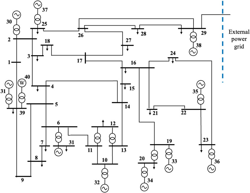
Figure 4. Modified IEEE 39-bus system.

Table 1

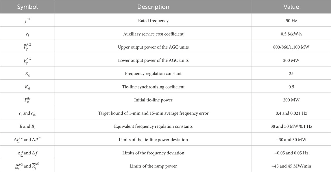
Table 1. Test system settings.

Figure 5

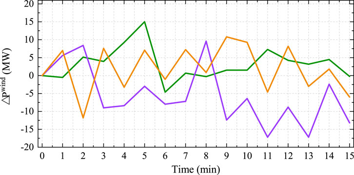
Figure 5. Wind power fluctuations in random periods.

For the agent settings, the discount factor $\gamma$ is set as 0.95 because the current power adjustment of the AGC units significantly impacts the future operating state of the system. The neural network structures of all the actor–critic networks are the same (i.e., $Q_{{\theta }_1}$, $Q_{{\theta }_2}$, $Q_{{\theta }_1^{\prime }}$, $Q_{{\theta }_2^{\prime }}$, and ${\pi }_{\varphi }$) and comprise two hidden layers of size $128\times 64.$ The smoothing factor for the two target networks is designed as $\beta$ = 0.01. Adam optimizer was adopted for gradient optimization with the learning rate ${\lambda }_{\alpha }$ = ${\lambda }_Q$ = 0.001. The three weight factors are set as $w_1$ = -0.05, $w_2$ = -1, and $w_3$ = -20. The replay buffer size $|\mathcal{D}|$ is set to 100,000. The introduced noise follows a Gaussian distribution of the form ${ϵ}_t\sim \mathcal{N}(0,1^2)$. The simulations were implemented in Python using an Intel Core i7 CPU @3.0 GHz and 16 GB memory.

In this work, we evaluated three benchmarks to validate the benefits of the proposed method: 1) proposed imitation-based SAC strategy denoted as ISAC; 2) traditional SAC strategy that uses the random initialization policy; 3) a classical proportional integral (PI) strategy. The PI strategy regulates the AGC units in proportion to the system frequency deviations. The following subsections show the results of both the training and control processes.

4.2 Offline and online training performances

The training process of the RL agent involves two stages: offline imitation learning and online RL training. The offline dataset is split into two subsets by random sampling, where 80% of the data are used for training and the remaining 20% are reserved for testing (i.e., validation). For the imitation network, the input data are the observed system state, and the label is the power regulation of the AGC units based on the classical PI strategy. This means that the final converged imitation policy is similar to the PI strategy. Figures 6, 7 show the imitation learning curves through the root mean-squared error (RMSE) and mean absolute error (MAE) indices. The black line represents the loss of the test dataset, and the red line represents the loss of the training dataset. It is observed that the training of the imitation network converges efficiently after approximately 200 epochs. Although the test loss is larger than the training loss initially, the converged strategy achieves training and test losses that are both less than 0.01. The training convergence is achieved at 10.04 s. These results indicate that the imitation learning process is both fast and stable, making it feasible for practical implementation.

Figure 6

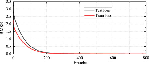
Figure 6. RMSE training results for imitation learning.

Figure 7

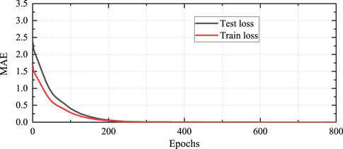
Figure 7. MAE training results for imitation learning.

To demonstrate the convergence of the proposed ISAC method, Figure 8 shows the cumulative reward of each episode through the blue lines and moving average reward via orange lines. It is seen that the episode reward decreases from −55 initially to approximately −15 after over 2,000 episodes, which implies successful convergence. Note that the cumulative reward of each episode still shows oscillations even after later training. This is because the wind power fluctuations are uncertain and vary widely over different periods, causing the optimal cost to be dynamic and inconstant. However, from the moving average curve, the episode reward is seen to decrease with continuous training until convergence.

Figure 8

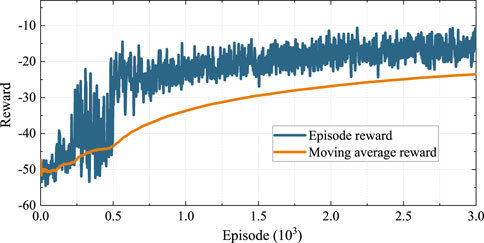
Figure 8. Episode reward for the proposed imitation-based SAC method.

To investigate the effects of the imitation network, we applied a random initialization policy in the SAC approach for comparison. Figure 9 shows the CPS1 training results based on two RL methods (i.e., SAC and ISAC). The blue line shows the CPS1 result for the ISAC method, and the orange line denotes the CPS1 result for the conventional SAC method. First, we see that the CPS1 results in both methods converge to 2 after 1,500 episodes. At the beginning of the training process, the value of the CPS1 index in the conventional SAC method is much lower than −2, with a minimum value of almost −12. This means that the system frequency stability is unacceptable for real-world grids. However, in the proposed ISAC method, the CPS1 result is always maintained within a small fluctuation range of [-2, 2] even at the beginning. This is because the proposed imitation network provides a satisfactory initialization policy by collecting effective samples for better policy optimization. It is noted that the sampling efficiency is sacrificed in the ISAC method to ensure safe exploration, where the CPS1 value is stable after approximately 1,500 episodes. In the conventional SAC method, the CPS1 value reaches 2 at nearly 1,000 episodes; this is because a large number of unsafe samples accelerate the learning process. Therefore, these results indicate that the proposed imitation network effectively prevents the unsafe random explorations observed in conventional RL methods, which can help cope with safety issues in real-world grids, especially for safety-critical AGC problems.

Figure 9

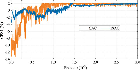
Figure 9. CPS1 training results of the RL agents.

4.3 System control performance

We applied two well-trained agents and a PI controller for comparison in the AGC environment. Figure 10 presents the system frequency fluctuations over 15 min with the same wind inputs based on the three control strategies, where the purple line denotes PI control, blue line denotes the SAC agent, and red line represents the proposed ISAC agent. At time step $t$ = 0, the initial frequency deviations are all 0. It is seen that the maximum frequency deviation of the PI controller is 0.076, which violates the upper limit of the frequency. However, the maximum values are only 0.045 and 0.028 in the SAC and proposed ISAC methods, respectively. This means that the two RL methods can adhere to the limits by effectively predicting wind fluctuations and taking actions in advance, with the proposed ISAC slightly outperforming the conventional SAC method with smaller frequency deviations.

Figure 10

Figure 10. System frequency fluctuations based on different strategies.

Table 2 presents a detailed comparison of the system control results, including the ancillary service costs, CPS1 index values, maximum frequency deviations, and average frequency deviations. We can see that the ancillary costs in the SAC and ISAC methods are significantly higher than that with the PI method because accurate responses to wind fluctuations require more power regulation in the AGC units. Correspondingly, the CPS1 values are effectively improved from 192.58% to 196.46% in the SAC and 199.27% in the proposed ISAC approaches. This means that there exists a tradeoff between the frequency stability and economic benefit depending on the system preference. In addition, the average frequency deviation with PI is 0.029, which decreases to 0.009 in the proposed ISAC to achieve a more stable system frequency. Hence, the converged SAC agent can also achieve satisfactory control results, with the main disadvantage being the unsafe training process. With the proposed imitation learning approach, the training process is safer and the final converged policy is improved through consideration of expert experiences. Figure 11 shows the AGC power regulation curves of the three AGC units. Although the regulation capacities and ramp limits are different, we can see that the curve trends for the three AGC units are quite similar. Specifically, for AGC units 1 and 2, the power deviations start at approximately −3 MW and decrease, reaching approximately −13 MW. At the end time, slight improvements are observed, with the deviations moving toward −5 MW. For AGC unit 3, the power deviation starts at approximately −5 MW and decreases to approximately −20 MW, showing more significant regulation than the other two units. This is because AGC unit 3 has the largest upper output power of 1,100 MW. In summary, all three AGC units experience significant negative power deviations initially, possibly owing to load changes or outdoor environment conditions, before recovering toward the end.

Table 2

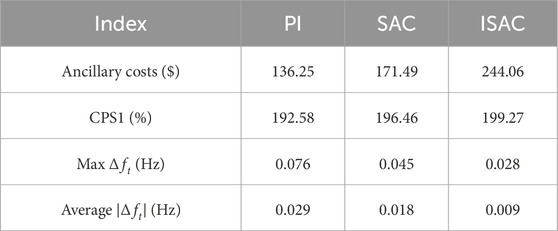
Table 2. Results of the three controllers.

Figure 11

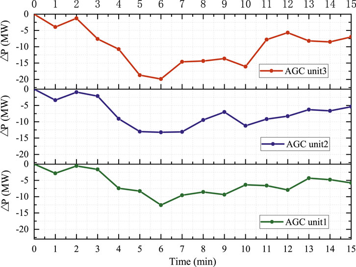
Figure 11. Power regulation results of the three AGC units.

5 Conclusion

To achieve real-time frequency response control, this work proposes an imitation-learning-based safe RL framework for AGC dynamic optimization. In the proposed method, an imitator is first used to effectively guarantee a safe initialization policy. Then, the AGC problem is reformulated as an MDP that is solved using an SAC algorithm combined with the imitator; the SAC approach is a model-free method that can handle wind power uncertainties through its forecasting capability. Finally, the proposed methodology is tested on a modified IEEE 39-bus system. The numerical results show that the proposed method effectively copes with stochastic disturbances and improves the CPS1 value from 192.58% to 199.27%. Meanwhile, compared to conventional RL methods, the proposed offline imitation learning achieves safer training performance by decreasing the constraint violations.

Data availability statement

The raw data supporting the conclusions of this article will be made available by the authors without undue reservation.

Author contributions

PY: writing–review and editing and writing–original draft. ZZ: writing–review and editing and writing–original draft. YW: writing–review and editing. ZH: writing–review and editing. MS: writing–review and editing.

Funding

The authors declare that financial support was received for the research, authorship, and/or publication of this article.

Conflict of interest

Authors ZZ, YW, ZH, and MS were employed by the State Grid Beijing Electric Power Company.

The remaining authors declare that the research was conducted in the absence of any commercial or financial relationships that could be construed as a potential conflict of interest.

The authors declare that this study received funding from the Science and Technology Project of State Grid Beijing Electric Power Company (grant number: 520210240001). The funder had the following involvement in the study: the writing of this article and the decision to submit it for publication.

Publisher’s note

All claims expressed in this article are solely those of the authors and do not necessarily represent those of their affiliated organizations or those of the publisher, editors, and reviewers. Any product that may be evaluated in this article or claim that may be made by its manufacturer is not guaranteed or endorsed by the publisher.

Abbreviations

AGC, automatic generation control; RL, reinforcement learning; ACE, area control error; CPS, control performance standard; NERC, North American Electric Reliability Council; PID, proportional integral derivative; SAC, soft actor–critic; MDP, Markov decision process; RMSE, root mean-squared error; BC, behavioral cloning; MSE, mean-squared error; KL, Kullback–Leibler; PI, proportional integral; MAE, mean absolute error.

Footnotes

¹When the discount factor $\gamma =0$, it means that the impact of the current decision on the future operating status of the system is not considered; when $\gamma =1$, it means that the impact of the current decision on the operating status of the system at every moment in the future is considered equally.

²https://www.iso-ne.com/isoexpress/web/reports.

References

Cheng, L., and Yu, T. (2019). A new generation of ai: a review and perspective on machine learning technologies applied to smart energy and electric power systems. Int. J. Energy Res. 43, 1928–1973. doi:10.1002/er.4333

CrossRef Full Text | Google Scholar

Daftry, S., Bagnell, J. A., and Hebert, M. (2017). “Learning transferable policies for monocular reactive mav control,” in 2016 international symposium on experimental robotics (Springer), 3–11. doi:10.1007/.978-3-319-50115-4_1

CrossRef Full Text | Google Scholar

Dahiya, P., Sharma, V., and Naresh, R. (2016). Automatic generation control using disrupted oppositional based gravitational search algorithm optimised sliding mode controller under deregulated environment. IET Generation, Transm. & Distribution 10, 3995–4005. doi:10.1049/iet-gtd.2016.0175

CrossRef Full Text | Google Scholar

Haarnoja, T., Zhou, A., Abbeel, P., and Levine, S. (2018). “Soft actor-critic: off-policy maximum entropy deep reinforcement learning with a stochastic actor,” in International conference on machine learning (PMLR), 1861–1870. Available at: https://proceedings.mlr.press/v80/haarnoja18b.html.

Google Scholar

Jaleeli, N., and VanSlyck, L. S. (1999). Nerc’s new control performance standards. IEEE Trans. Power Syst. 14, 1092–1099. doi:10.1109/59.780932

CrossRef Full Text | Google Scholar

Kumar, N. (2024). Ev charging adapter to operate with isolated pillar top solar panels in remote locations. IEEE Trans. Energy Convers. 39, 29–36. doi:10.1109/TEC.2023.3298817

CrossRef Full Text | Google Scholar

Kumar, N., Saxena, V., Singh, B., and Panigrahi, B. K. (2023a). Power quality improved grid-interfaced pv-assisted onboard ev charging infrastructure for smart households consumers. IEEE Trans. Consum. Electron. 69, 1091–1100. doi:10.1109/TCE.2023.3296480

CrossRef Full Text | Google Scholar

Kumar, N., Singh, H. K., and Niwareeba, R. (2023b). Adaptive control technique for portable solar powered ev charging adapter to operate in remote location. IEEE Open J. Circuits Syst. 4, 115–125. doi:10.1109/.OJCAS.2023.3247573

CrossRef Full Text | Google Scholar

Li, J., Yu, T., Zhang, X., Li, F., Lin, D., and Zhu, H. (2021). Efficient experience replay based deep deterministic policy gradient for agc dispatch in integrated energy system. Appl. energy 285, 116386. doi:10.1016/j.apenergy.2020.116386

CrossRef Full Text | Google Scholar

Liu, Z., Li, J., Zhang, P., Ding, Z., and Zhao, Y. (2022). An agc dynamic optimization method based on proximal policy optimization. Front. Energy Res. 10, 947532. doi:10.3389/fenrg.2022.947532

CrossRef Full Text | Google Scholar

Oshnoei, A., Kheradmandi, M., Khezri, R., and Mahmoudi, A. (2020). Robust model predictive control of gate-controlled series capacitor for lfc of power systems. IEEE Trans. Ind. Inf. 17, 4766–4776. doi:10.1109/TII.2020.3016992

CrossRef Full Text | Google Scholar

Peddakapu, K., Mohamed, M., Srinivasarao, P., Arya, Y., Leung, P., and Kishore, D. (2022). A state-of-the-art review on modern and future developments of agc/lfc of conventional and renewable energy-based power systems. Renew. Energy Focus 43, 146–171. doi:10.1016/j.ref.2022.09.006

CrossRef Full Text | Google Scholar

Rajaraman, N., Yang, L., Jiao, J., and Ramchandran, K. (2020). Toward the fundamental limits of imitation learning. Adv. Neural Inf. Process. Syst. 33, 2914–2924.

Google Scholar

Ruan, J., Liang, G., Zhao, H., Liu, G., Sun, X., Qiu, J., et al. (2024). Applying large language models to power systems: potential security threats. IEEE Trans. Smart Grid 15, 3333–3336. doi:10.1109/TSG.2024.3373256

CrossRef Full Text | Google Scholar

Sahu, B. K., Pati, S., Mohanty, P. K., and Panda, S. (2015). Teaching–learning based optimization algorithm based fuzzy-pid controller for automatic generation control of multi-area power system. Appl. Soft Comput. 27, 240–249. doi:10.1016/j.asoc.2014.11.027

CrossRef Full Text | Google Scholar

Satapathy, S. S., and Kumar, N. (2020). Framework of maximum power point tracking for solar pv panel using wsps technique. IET Renew. Power Gener. 14, 1668–1676. doi:10.1049/iet-rpg.2019.1132

CrossRef Full Text | Google Scholar

Wang, C., Zhu, J., and Zhu, T. (2018). “Decentralized robust optimization for real-time dispatch of power system based on approximate dynamic programming,” in 2018 international conference on power system Technology (POWERCON) (IEEE), 1935–1941. doi:10.1109/POWERCON.2018.8601952

CrossRef Full Text | Google Scholar

Wang, X., Wang, S., Liang, X., Zhao, D., Huang, J., Xu, X., et al. (2022). Deep reinforcement learning: a survey. IEEE Trans. Neural Netw. Learn. Syst. 35, 5064–5078. doi:10.1109/TNNLS.2022.3207346

CrossRef Full Text | Google Scholar

Wang, Y., Lin, X., Tan, Z., Liu, Y., Song, Z., Yu, L., et al. (2023). “Wind power forecasting: lstm-combined deep reinforcement learning approach,” in 2023 IEEE 7th conference on energy internet and energy system integration (EI2) (IEEE), 5202–5206. doi:10.1109/EI259745.2023.10512354

CrossRef Full Text | Google Scholar

Wang, Z., and Zhang, H. (2024). Customized load profiles synthesis for electricity customers based on conditional diffusion models. IEEE Trans. Smart Grid 15, 4259–4270. doi:10.1109/TSG.2024.3366212

CrossRef Full Text | Google Scholar

Wu, Z., Shen, Y., Pan, T., and Ji, Z. (2010). “Feedback linearization control of pmsm based on differential geometry theory,” in 2010 5th IEEE conference on industrial electronics and applications (IEEE), 2047–2051. doi:10.1109/ICIEA.2010.5515457

CrossRef Full Text | Google Scholar

Xi, L., Zhou, L., Liu, L., Duan, D., Xu, Y., Yang, L., et al. (2020). A deep reinforcement learning algorithm for the power order optimization allocation of agc in interconnected power grids. CSEE J. Power Energy Syst. 6, 712–723. doi:10.17775/CSEEJPES.2019.01840

CrossRef Full Text | Google Scholar

Yan, W., Zhao, R.-F., Zhao, X., Wang, C., and Yu, J. (2013). Review on control strategies in automatic generation control. Power Syst. Prot. control 41, 149–155.

Google Scholar

Yang, L., Liang, G., Yang, Y., Ruan, J., Yu, P., and Yang, C. (2024). Adversarial false data injection attacks on deep learning-based short-term wind speed forecasting. IET Renew. Power Gener. 18, 1370–1379. doi:10.1049/rpg2.12853

CrossRef Full Text | Google Scholar

Yu, P., Wang, Z., Zhang, H., and Song, Y. (2024a). Safe reinforcement learning for power system control: a review. arXiv Prepr. arXiv:2407.00681. doi:10.48550/arXiv.2407.00681

CrossRef Full Text | Google Scholar

Yu, P., Zhang, H., and Song, Y. (2024b). Adaptive tie-line power smoothing with renewable generation based on risk-aware reinforcement learning. IEEE Trans. Power Syst., 1–13. doi:10.1109/TPWRS.2024.3379513

CrossRef Full Text | Google Scholar

Zhang, J., Lu, C., Song, J., and Zhang, J. (2015). Real-time agc dispatch units considering wind power and ramping capacity of thermal units. J. Mod. Power Syst. Clean Energy 3, 353–360. doi:10.1007/s40565-015-0141-z

CrossRef Full Text | Google Scholar

Zhang, R., Chen, Y., Li, Z., Jiang, T., and Li, X. (2024). Two-stage robust operation of electricity-gas-heat integrated multi-energy microgrids considering heterogeneous uncertainties. Appl. Energy 371, 123690. doi:10.1016/j.apenergy.2024.123690

CrossRef Full Text | Google Scholar

Zhang, X., Xu, Z., Yu, T., Yang, B., and Wang, H. (2020). Optimal mileage based agc dispatch of a genco. IEEE Trans. Power Syst. 35, 2516–2526. doi:10.1109/TPWRS.2020.2966509

CrossRef Full Text | Google Scholar

Zhao, X., Ye, X., Yang, L., Zhang, R., and Yan, W. (2019). Chance constrained dynamic optimisation method for agc units dispatch considering uncertainties of the offshore wind farm. J. Eng. 2019, 2112–2119. doi:10.1049/joe.2018.8558

CrossRef Full Text | Google Scholar

Zheng, Y., Tao, J., Sun, H., Sun, Q., Chen, Z., Dehmer, M., et al. (2021). Load frequency active disturbance rejection control for multi-source power system based on soft actor-critic. Energies 14, 4804. doi:10.3390/.en14164804

CrossRef Full Text | Google Scholar