Dynamic prediction of overhead transmission line ampacity based on the BP neural network using Bayesian optimization

Traditionally, the ampacity of an overhead transmission line (OHTL) is a static value obtained based on adverse weather conditions, which constrains the transmission capacity. With the continuous growth of power system load, it is increasingly necessary to dynamically adjust the ampacity based on weather conditions. To this end, this paper models the heat balance relationship of the OHTL based on a BP neural network using Bayesian optimization (BO-BP). On this basis, an OHTL ampacity prediction method considering the model error is proposed. First, a two-stage current-stepping ampacity prediction model is established to obtain the initial ampacity prediction results. Then, the risk control strategy of ampacity prediction considering the model error is proposed to correct the ampacity based on the quartile of the model error to reduce the risk of the conductor overheating caused by the model error. Finally, a simulation is carried out based on the operation data of a 220-kV transmission line. The simulation results show that the accuracy of the BO-BP model is improved by more than 20% compared with the traditional heat balance equation. The proposed ampacity prediction method can improve the transmission capacity by more than 150% compared with the original static ampacity.

1 Introduction

An overhead transmission line (OHTL) is a necessary link in the transmission of electrical energy, and its capacity determines the transmission capacity of the grid. In recent years, there has been a gradual increase in power loads, and grid congestion has intensified (Ahmadi et al., 2023). High penetration of renewable energy places higher demands on the transmission capacity of the grid (Lebedov et al., 2021; Lawal and Teh, 2023b). The fundamental way to increase the transmission capacity of the grid is to build new OHTLs. However, this method takes a long time and cannot meet the current power load demand (Madadi et al., 2020). Therefore, there is a need to tap the transmission potential of the OHTL in the short term. An important indicator for assessing the capacity of an OHTL is ampacity, which is the maximum wire current calculated based on the weather conditions around the OHTL and the maximum permissible conductor temperature (Bao et al., 2015). Current OHTL design specifications typically use static ampacity (Jabarnejad, 2015). The principle of static ampacity is to assume extremely adverse cooling conditions and calculate a conservative ampacity through standards such as IEEE-738 and CIGRE (Morozovska and Hilber, 2017; Kanálik et al., 2019; Su et al., 2022). Continuing to limit the capacity of the OHTL through static ampacity will make it difficult to meet the transmission needs of the grid (Chen et al., 2017).

Weather conditions determine the heat dissipation capacity of the OHTL and, hence, ampacity. Therefore, ampacity can be dynamically adjusted by obtaining real-time weather conditions around the OHTL. Currently, there are three main methods to dynamically acquire ampacity. The first method is to install a weather monitoring device near the OHTL to collect weather information, then transmit the weather data to a computer through wireless communication technology, and then substitute them into the heat balance equation to calculate the real-time ampacity (Douglass and Edris, 1996; Bhattarai et al., 2018). The second method is to analyze the temporal and spatial correlation of the weather data to indirectly obtain the weather data and then obtain the ampacity based on the heat balance equation (Fan et al., 2015; Fernandez et al., 2015; Sun et al., 2019; Alberdi et al., 2022; Karimi et al., 2022; Zhang et al., 2024). The last method is to use machine learning algorithms to establish the heat balance relationship of OHTLs and, thus, calculate ampacity (Morrow et al., 2014; Jin et al., 2020; Molinar et al., 2021; Sobhy et al., 2021).

Regarding the first method, in a project conducted by the Electric Power Research Institute, weather data were collected through weather stations, digital data loggers, and IBM-compatible PCs to calculate the ampacity of multiple OHTLs (Douglass and Edris, 1996). Furthermore, the ampacity prediction system developed by the Idaho National Laboratory considers the effect of the geographic location of weather stations to determine the optimal number and location of weather stations (Bhattarai et al., 2018). The above methods require the installation of a large number of weather collection devices. The cost of the system is high, and the reliability is low.

The second option aims at avoiding the installation of weather collection devices. Fernandez et al. (2015) applied numerical weather prediction to ampacity prediction. Alberdi et al. (2022); Karimi et al. (2022); and Zhang et al. (2024) developed time series prediction models for weather conditions. However, temporal weather forecasts do not consider spatial differences in weather conditions. Spatial interpolation methods such as Kriging and IDW compensate for this deficiency (Fan et al., 2015; Sun et al., 2019). The above methods still rely on the heat balance equation for calculating ampacity. Due to certain engineering approximations in the heat balance equation, it may be difficult to accurately reflect the heat balance relationship of the OHTL.

Machine learning algorithms have good prospects in the field of ampacity prediction due to their good modeling capabilities. Morrow et al. (2014) used a partial least squares regression algorithm for modeling, but this approach was limited to linear models. Algorithms such as random forests and neural networks, on the other hand, do not restrict the form of the objective function and offer more flexibility (Jin et al., 2020; Sobhy et al., 2021). Incremental learning based on real-time data allows the model to be updated in real time, thus improving the model’s adaptivity and computational efficiency (Molinar et al., 2021). However, machine learning algorithms often have some hyperparameters that need to be set manually. Research on hyperparameter optimization is rarely mentioned. The optimization of hyperparameters is meaningful to improve the training effect.

In order to solve the problem of the low accuracy of the heat balance equation in ampacity calculation, we establish the heat balance relationship model of the OHTL based on the BP neural network using the Bayesian optimization (BO-BP) algorithm. On this basis, we set a safety margin based on the lower α-quantile of the model error, which improves the reliability of the results of the ampacity calculation. The main contributions of this paper are as follows:

1) The heat balance relationship of the OHTL is established based on the BO-BP. The BP neural network is used for regression analysis between weather conditions, wire current, and conductor temperature. Bayesian optimization is used to optimize the hyperparameters of the BP neural network.

2) A two-stage current-stepping ampacity prediction model is proposed. The model combines the BO-BP algorithm with the heat balance equation. When weather conditions are known, the conductor temperature is calculated in two stages based on wire current values. The wire current is iteratively increased until the conductor temperature exceeds a set value, and then ampacity is obtained based on linear interpolation.

3) A risk control strategy for ampacity prediction is proposed taking into account the model error. Based on the quartile of the model error, the results of ampacity are corrected to reduce the risk of conductor overheating caused by the model error. The impact of different quartile values on the capacity improvement effect is analyzed.

2 Heat balance relationship model of the OHTL

2.1 Heat balance equation

The heat balance equation is the physical model reflecting the heat balance relationship of the OHTL, and its steady state form is as follows:

$P_J+P_S=P_C+P_R(1)$

where P_J is the Joule heat power generated by the wire current; P_S is the heat absorption power of solar radiation; P_C is the convective heat dissipation power; and P_R is the radiant heat dissipation power. Their specific formulas are as follows:

$\left\{\begin{array}{l}{P}_J=I^{2}R\\ P_S=a_S{I}_{S}D\\ P_C=9.92\left(T-T_A\right){\left(VD\right)}^{0.485}\\ P_R=\pi eSD\left[{\left(T+273\right)}^4-{\left(T_A+273\right)}^4\right]\end{array}\right.(2)$

where I is the wire current; R is the AC resistance per unit length of the transmission line; a_S is the heat absorption coefficient; I_S is the solar irradiance; D is the outer diameter of the conductor; T is the conductor temperature; T_A is the ambient temperature; V is the equivalent wind speed; e is the heat dissipation coefficient; and S is the Stefan–Boltzmann constant. The expression for R is

$R=I^{\tau }\zeta R_{20}\left[1+\beta \left(T-20\right)\right](3)$

where τ and ζ are related to the AC/DC resistance ratio, which is determined according to the type of the transmission line. R₂₀ is the DC resistance per unit length at 20°C. β is the temperature coefficient of resistance.

Considering the effect of wind direction, the equivalent wind speed V is expressed as follows:

$V=v\left(1.194-\cos \phi +0.194\cos 2\phi +0.368\sin 2\phi \right)(4)$

where v is the wind speed and φ is the angle made by the wind with the transmission line.

According to Equations 1, 2, the formula for ampacity is as follows:

$I=\sqrt{\frac{P_C+P_R-P_S}{R}}(5)$

2.2 BO-BP algorithm

2.2.1 BP neural networks

The BP neural network is used in this paper to establish the relationship between weather conditions, wire current, and conductor temperature. The input variables are wind speed v, wind direction θ, solar irradiance I_S, ambient temperature T_A, and wire current I. The output variable is conductor temperature T. The BP neural network consists of three layers: an input layer, a hidden layer, and an output layer. The input layer receives the data, the output layer outputs the result, and the hidden layer is used to establish complex relationships. The operation mechanism of the BP neural network consists of two parts: forward propagation and backpropagation.

Forward propagation uses the output of the previous layer as the input of the current layer, calculating the output for the current layer through weighted summation and activation function transformation until reaching the output layer. Assuming that the output of the previous layer is y_l-1, the output of the current layer is shown in Equation 6:

$y_l=\sigma \left(W{y}_{l-1}+b\right)(6)$

The hyperbolic tangent function is used for the activation function σ. W is the weight matrix. b is the offset vector.

The principle of backpropagation is to first compute the loss function based on the output layer results obtained from forward propagation. Then, the gradient of the loss function with respect to W and b is calculated. Finally, the optimal W and b are found based on optimization algorithms, such as gradient descent. In this paper, the loss function used is the mean square error (MSE) function, and the optimization algorithm is the Levenberg–Marquardt (Wilamowski and Hao Yu, 2010).

2.2.2 Bayesian optimization

In this study, the BP neural network uses a single-hidden layer structure. There are two pre-set hyperparameters, namely, learning rate and the number of neurons in the hidden layer, and they will be obtained using the Bayesian optimization algorithm.

Bayesian optimization is a hyperparametric search method. The Bayesian optimization algorithm establishes a Gaussian process regression model based on existing observations to estimate the potential distribution of the objective function. The acquisition function is used to select the hyperparameters for the next iteration until the stopping condition is satisfied. Since Bayesian optimization utilizes the previous search results, it has higher search efficiency than grid search and random search. The principle is shown in Figure 1.

Figure 1

Figure 1. Principle of the BO-BP algorithm.

2.3 Evaluation metrics for model accuracy

The root mean square error (RMSE) of the conductor temperature is used to evaluate the accuracy of the BO-BP model and the heat balance equation. The RMSE is calculated by Equation 7:

$\text{RMSE}=\sqrt{\frac{{\displaystyle \sum _{i=1}^n}{\left(T_{ri}-T_{\mathrm{c}i}\right)}^2}{n}}(7)$

where T_ri is the true value of conductor temperature; T_ci is the calculated value of conductor temperature; and n is the number of samples.

In this study, the heat balance equation is the baseline model. The RMSE reduction ratio ΔR₁₂ is used to evaluate the accuracy improvement effect of the BO-BP algorithm, which is defined as Equation 8:

$\Delta R_{12}=\frac{R_1-R_2}{R_1}\times 100\%(8)$

where R₁ is the RMSE of the heat balance equation and R₂ is the RMSE of the BO-BP algorithm.

3 OHTL ampacity prediction method considering the model error

3.1 Two-stage current-stepping ampacity prediction model

According to Chinese design regulations, the maximum conductor temperature for long-term operation is 70°C (Song et al., 2019). However, the conductor temperature rarely reaches this value during actual operation. This is the main challenge in calculating ampacity using the BO-BP algorithm. To solve this problem, a two-stage current-stepping ampacity prediction model is proposed, which combines the BO-BP algorithm with the heat balance equation. The principle is as follows.

When the weather conditions are known, the wire current I is continuously increased, and the conductor temperature T is calculated until T > 70°C; thus, an I-T curve is obtained, and then, the ampacity at 70°C is obtained by linear interpolation. Let the minimum value of the wire current of the training set be I₁ and the maximum value be I_k. The first stage is when I₁ ≤ I ≤ I_k, and the second stage is when I > I_k.

In the first stage, the initial value of the wire current is set to I₁. The conductor temperature T₁ is calculated based on the BO-BP algorithm, and the wire current is increased in a step size of ΔI₁ until I = I_k or the conductor temperature is higher than 70°C. Thus, the iterative equation for the first stage is shown in Equation 9:

$\left\{\begin{array}{l}{I}_i=I_{i-1}+\Delta I_1\\ T_i=F\left(v,\theta ,I_S,T_A,I_i\right)\end{array}\right.(9)$

where I_i-1 is the wire current from the previous iteration and F is the trained BO-BP model. If the conductor temperature T_i > 70°C during the iteration, ampacity is calculated according to the linear interpolation method using the following expression:

$I_{DA}=I_{i-1}+\frac{I_i-I_{i-1}}{T_i-T_{i-1}}\left(70-T_{i-1}\right)(10)$

where T_i-1 is the conductor temperature from the previous iteration.

If the conductor temperature does not exceed 70°C in the first stage, the second stage is entered. In the second stage, since the wire current exceeds the range of values of the training set, the conductor temperature is calculated according to the heat balance equation. The heat balance equation is corrected according to the results of the last iteration of the first stage so that the iterative equation of the second stage is shown in Equation 11:

$\left\{\begin{array}{l}{I}_i=I_{i-1}+\Delta I_2\\ T_i=g\left(v,\theta ,I_S,T_A,I_i\right)+T_k-g\left(v,\theta ,I_S,T_A,I_k\right)\end{array}\right.(11)$

where ΔI₂ is the step size of the wire current in the second stage; T_k is the conductor temperature obtained from the last iteration of the first stage; and g is the heat balance equation. Ampacity is calculated according to Equation 10 when T_i > 70°C. Figure 2 shows the flowchart of the two-stage current-stepping ampacity prediction model.

Figure 2

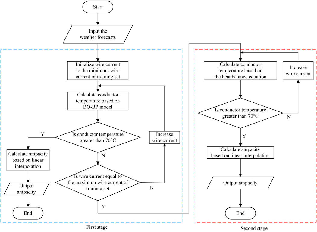
Figure 2. Flowchart of the two-stage current-stepping ampacity prediction model.

3.2 Risk control strategy for ampacity prediction considering the model error

The BO-BP algorithm has some uncertainty. This poses a challenge to the accuracy of dynamic ampacity prediction. The risk can be predicted based on the statistical analysis of the historical model error. The expression for the model error is shown in Equation 12:

$T_E=T_R-T_C(12)$

where T_R is the true value of the conductor temperature of the test set and T_C is the calculated value of the conductor temperature of the test set. When the model error T_E > 0, it is called a positive model error, indicating that the true value of the conductor temperature is higher than the calculated value, which will yield overly optimistic ampacity prediction results. In order to reduce the probability of a positive model error occurring, the initial I–T curve is shifted upward by ΔT_α unit lengths. ΔT_α is the lower α-quantile of the model error and is defined as Equation 13:

$P\left(T_E<\Delta T_{\alpha }\right)=\alpha (13)$

The calculation process is as follows:

1) The model errors of the test set are sorted from smallest to largest, and let the ith element be $T_E^i$.

2) The element number pos corresponding to α is calculated. The formula is shown in Equation 14:

$pos=1+\left(n-1\right)\alpha (14)$

where n is the number of samples in the test set.

3) Since pos is not necessarily an integer, ΔT_α needs to be obtained by linearly interpolating the two model error elements adjacent to pos, calculated by Equation 15:

$\left\{\begin{array}{l}\Delta T_{\alpha }=T_E^{low}+\frac{T_E^{high}-T_E^{low}}{high-low}\left(pos-low\right)\\ low=\lfloor pos\rfloor \\ high=\lceil pos\rceil \end{array}\right.(15)$

where $\lfloor pos\rfloor$ is the largest integer not exceeding pos and $\lceil pos\rceil$ is the smallest integer not less than pos.

Figure 3 shows the principle of the risk control strategy for ampacity prediction considering the model error.

Figure 3

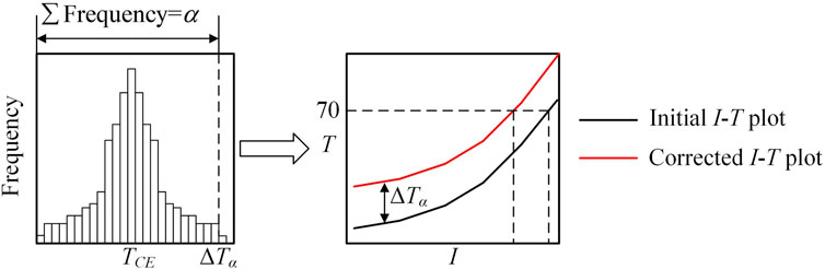
Figure 3. Risk control strategy for ampacity prediction considering the model error.

3.3 Evaluation metrics for capacity improvement

The average capacity improvement ratio is used to evaluate the improvement effect of the ampacity calculated in this paper compared to the static ampacity. It is defined as Equation 16:

$r_{DS}=\frac{1}{n}{\displaystyle \sum _{i=1}^n}\frac{I_{DAi}-I_{SA}}{I_{SA}}(16)$

where n is the number of samples; I_DAi is the ampacity calculated by the method described in this paper; I_SA is the static ampacity of the line, and its value is 581 A.

4 Case study

The study is based on operational data of a 220-kV OHTL. First, the weather, wire current, and conductor temperature are statistically analyzed based on the operational data from 2022. Then, the BO-BP model is trained. The dataset is divided into a training set, a validation set, and a test set in a ratio of 3:1:1. The training set is used to train the BP neural network model, the validation set is utilized for Bayesian optimization of hyperparameters, and the test set is utilized to evaluate the model’s accuracy as well as error analysis. Finally, the improvement effect of ampacity is evaluated based on 2023 weather data, and the effect of different quantile values on the ampacity results is analyzed.

4.1 Statistical analysis of historical data

4.1.1 Statistical analysis of weather conditions

The weather elements considered in this study are wind speed v, wind direction θ, solar irradiance I_S, and ambient temperature T_A. θ is transformed to the range of [0°,180°] due to the equivalent heat dissipation effect on the conductor when the wind directions differ by 180°. The north–south direction is 0°, and the clockwise direction is positive. December, January, and February are classified as winter, while March, April, and May are classified as spring. The months of June, July, and August are classified as summer. The months of September, October, and November are classified as fall. Figure 4 illustrates the distribution of each weather element for the four seasons.

Figure 4

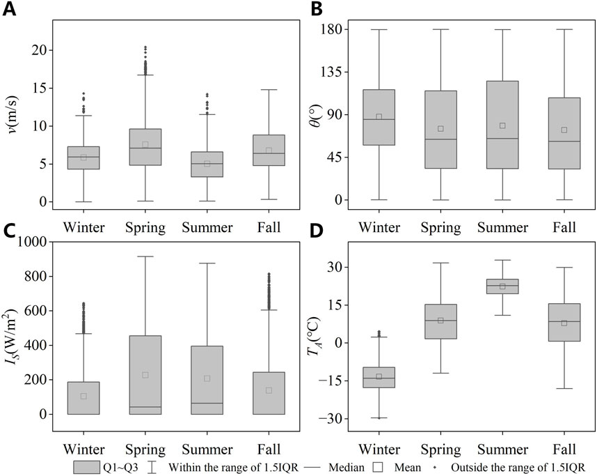
Figure 4. Distribution of each weather element for the four seasons. (A) Wind speed. (B) Wind direction. (C) Solar irradiance. (D) Ambient temperature.

As shown in Figure 4, wind speeds are generally lower in winter and summer than in spring and fall. The difference in wind direction between the four seasons is minimal. Solar irradiance is generally higher in spring and summer than in winter and fall. The four-season difference in ambient temperature is most pronounced. Winter temperatures are predominantly below 0°C. The temperature range in spring and fall is more extensive, with lows in the vicinity of −15°C and highs reaching 30°C. Temperatures in summer are mostly above 15°C.

4.1.2 Statistical analysis of wire current and conductor temperature

The distributions of conductor temperature and wire current in four seasons are shown in Figure 5.

Figure 5

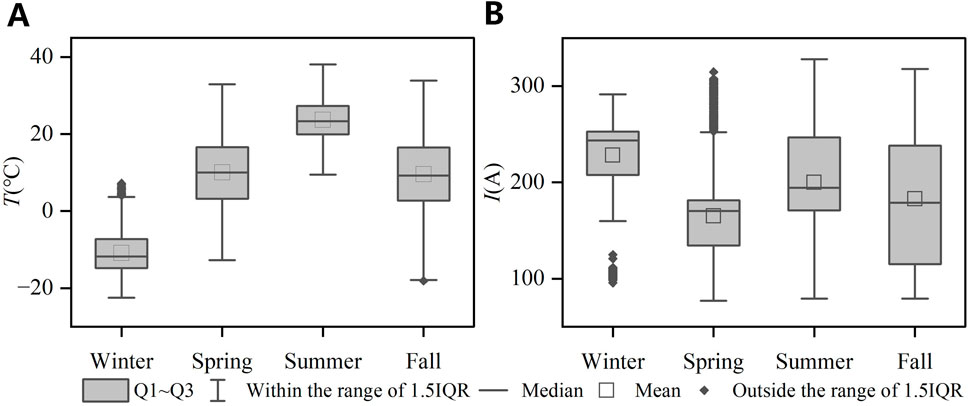
Figure 5. Conductor temperature and wire current distribution for the four seasons. (A) Conductor temperature. (B) Wire current.

It can be observed that the distribution characteristics of the conductor temperature are largely consistent with the ambient temperature. The majority of wire currents in the four seasons range from 100 A to 300 A. It can be noted that wire currents in winter are generally higher than those in the other three seasons, followed by summer and fall, and lowest in spring.

4.2 Heat balance equation results

The type of the OHTL used in this study is LGJ400/35. Its design parameters are shown in Table 1.

Table 1

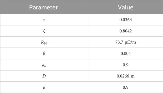
Table 1. Parameters of LGJ400/35.

The conductor temperature is calculated by substituting the weather conditions and wire current of the test set into the heat balance equation. The calculated values of conductor temperature are obtained by solving the quartic equation for T using Equations 1–4. The true value of the conductor temperature is measured by a temperature sensor on the OHTL. The comparison of the calculated values with the true values is shown in Figure 6.

Figure 6

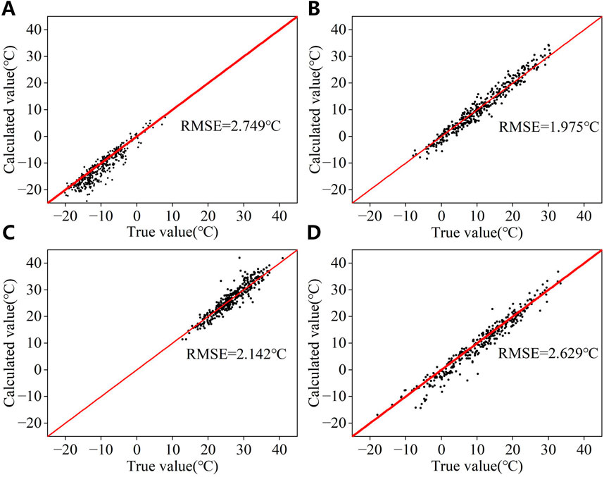
Figure 6. Calculated and true values of conductor temperature for the heat balance equation for the four seasons. (A) Winter. (B) Spring. (C) Summer. (D) Fall.

As shown in Figure 6, the RMSE of the heat balance equation is considerably higher in winter and fall than in spring and summer. With the exception of spring, a considerable number of samples exhibit significant errors in all three seasons.

4.3 BO-BP algorithm results

The BO-BP model is trained based on the data of training and validation sets. Subsequently, the weather conditions and wire current of the test set are substituted into the BO-BP model to obtain the calculated values of conductor temperature. A comparison of the calculated and true values is shown in Figure 7. The RMSE reduction ratio ΔR₁₂ compared to the heat balance equation is shown in Table 2:

Figure 7

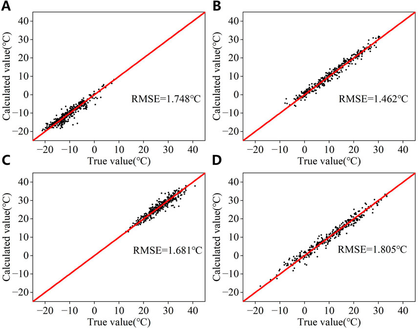
Figure 7. Calculated and true values of conductor temperature for the BO-BP algorithm for the four seasons. (A) Winter. (B) Spring. (C) Summer. (D) Fall.

Table 2

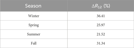
Table 2. RMSE reduction ratio ΔR₁₂ compared to the heat balance equation.

As shown in Figure 7 and Table 2, the BO-BP algorithm exhibits enhanced accuracy compared to the heat balance equation across all seasons. The number of samples exhibiting significant errors has decreased. This improvement is particularly pronounced in winter and fall. Nevertheless, a small number of samples still exhibit considerable model errors in winter and summer.

4.4 Results of statistical analysis of the model error

The model error of the BO-BP algorithm is statistically analyzed. The frequency histograms for the four seasons are shown in Figure 8.

Figure 8

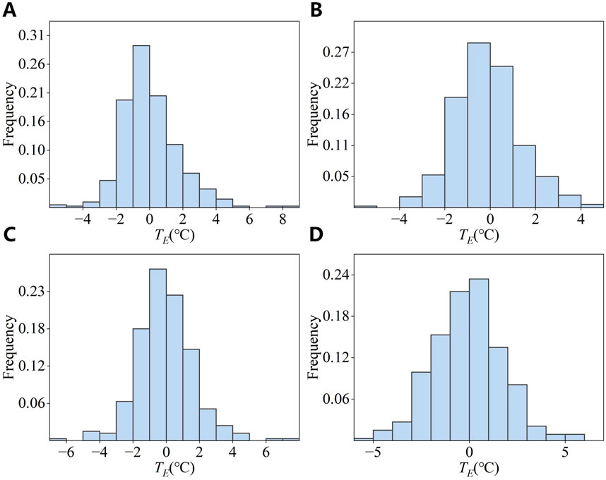
Figure 8. Frequency histograms of model errors of the BO-BP algorithm for the four seasons. (A) Winter. (B) Spring. (C) Summer. (D) Fall.

As shown in Figure 8, the majority of the model errors for the four seasons are concentrated near 0°C, with a small number of samples exhibiting considerable errors. The corresponding ΔT_α values for different α values are shown in Figure 9.

Figure 9

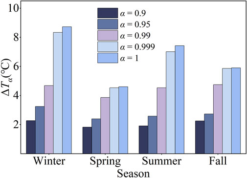
Figure 9. ΔT_α values corresponding to different α values.

As shown in Figure 9, a larger α value corresponds to a larger ΔT_α value. When α ≤ 0.99, the trends of ΔT_α for the four seasons are comparable. When α ≥ 0.999, ΔT_α of the four seasons exhibits a significant discrepancy, i.e., higher in winter and summer and lower in spring and fall. This discrepancy can be attributed to the presence of a considerable degree of error in a small number of samples in the winter and summer.

4.5 Results of the dynamic ampacity prediction

The initial ampacity I_DA is calculated based on the weather data from 2023, and the reduction in ampacity ΔI_α is analyzed for different values of α. The results are shown in Figure 10.

Figure 10

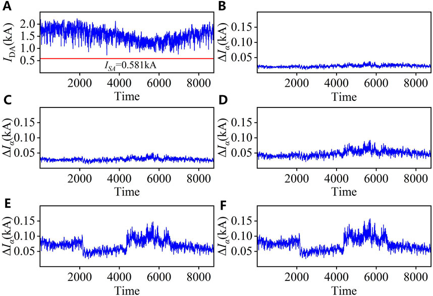
Figure 10. Results of initial ampacity and ΔI_α. (A) Initial ampacity. (B) ΔI_α at α = 0.90. (C) ΔI_α at α = 0.95. (D) ΔI_α at α = 0.99. (E) ΔI_α at α = 0.999. (F) ΔI_α at α = 1.

As shown in Figure 10A, the initial ampacity results are consistently higher than the static ampacity results throughout 2023. The ampacity results exhibit a seasonal distribution pattern, with the highest values observed in winter, a gradual decrease in spring, the lowest values observed in summer, and a gradual increase in fall. Figures 10B–F show that ΔI_α demonstrates a gradual increase as α increases. When α ≤ 0.99, ΔI_α exhibits a relatively consistent pattern throughout the year. When α ≥ 0.999, ΔI_α is significantly larger in winter and summer than in spring and fall. These results indicate that the risk control strategy in this paper sets the safety margin of ampacity based on the statistical analysis of historical model errors. The average capacity improvement ratio results are listed in Table 3.

Table 3

Table 3. Average capacity improvement ratio for different scenarios.

As shown in Table 3, the larger α is, the smaller R_DS is. When α = 1, the R_DS still reaches 154.79%. Consequently, by incorporating the index of α, the risk of conductor overheating due to the model error can be mitigated while maintaining the capacity improvement effect.

5 Conclusion

Aiming at the problem that static ampacity is difficult to meet the power supply demand, this study proposes a dynamic ampacity prediction scheme. The heat balance relationship of the OHTL is modeled based on the BO-BP algorithm. On this basis, an OHTL ampacity prediction method considering the model error is proposed. The method of this paper is validated based on the operational data of a 220-kV OHTL, and the results show that

1) The proposed BO-BP algorithm shows a significant improvement in accuracy compared to the heat balance equation, and the RMSE reduction ratio can reach more than 20%.

2) The method in this paper dynamically adjusts the ampacity according to weather conditions and takes into account the risk associated with model errors. The OHTL capacity can be improved by more than 150% compared to using static ampacity.

In this study, an offline-trained BO-BP model is constructed based on historical data from the OHTL. The offline-trained model may become less adaptable as the running time passes. Therefore, future research is directed toward online training of ampacity prediction based on real-time data. Moreover, dynamic adjustment of ampacity leads to an increase in conductor temperature, and the resulting faster rate of aging and increase in the rate of line failure are issues that need to be investigated (Teh et al., 2017; Teh, 2018). In addition, the interconnectivity of communication devices and data integrity need to be considered during the actual system development process, which will enhance the reliability, operation, and deployability of the system (Jimada-Ojuolape and Teh, 2020; Jimada-Ojuolape and Teh, 2022a; Jimada-Ojuolape and Teh, 2022b; Jimada-Ojuolape et al., 2023; Lawal and Teh, 2023a; Jimada-Ojuolape et al., 2024; Lawal et al., 2024).

Data availability statement

The raw data supporting the conclusion of this article will be made available by the authors, without undue reservation.

Author contributions

YS: funding acquisition, methodology, writing–original draft, and writing–review and editing. YLi: investigation and writing–review and editing. BW: conceptualization and writing–review and editing. YLu: investigation and writing–review and editing. RF: formal analysis and writing–review and editing. XS (6th author): resources and writing–review and editing. YJ: software and writing–review and editing. XS (8th author): data curation and writing–review and editing. SS: data curation and writing–review and editing. KM: validation and writing–review and editing. GZ: project administration and writing–review and editing. XS (12th author): visualization and writing–review and editing.

Funding

The author(s) declare that financial support was received for the research, authorship, and/or publication of this article. This research was funded by State Grid Jilin Sheng Electric Power Supply Company, grant number SGJLJY00GPJS2200077.

Conflict of interest

Authors YS, XS (6th author), and YJ were employed by State Grid Jilin Sheng Electric Power Supply Company. Authors YLi, BW, YLu, XS (8th author), SS, and KM were employed by Power Economic Research Institute of Jilin Electric Power Co., Ltd.

The remaining authors declare that the research was conducted in the absence of any commercial or financial relationships that could be construed as a potential conflict of interest.

The authors declare that this study received funding from State Grid Jilinsheng Electric Power Supply Company. The funder had the following involvement in the study: the data collection and analysis part.

Publisher’s note

All claims expressed in this article are solely those of the authors and do not necessarily represent those of their affiliated organizations, or those of the publisher, the editors, and the reviewers. Any product that may be evaluated in this article, or claim that may be made by its manufacturer, is not guaranteed or endorsed by the publisher.

References

Ahmadi, A., Taheri, S., Ghorbani, R., Vahidinasab, V., and Mohammadi-ivatloo, B. (2023). Decomposition-based stacked bagging boosting ensemble for dynamic line rating forecasting. IEEE Trans. Power Deliv. 38, 2987–2997. doi:10.1109/TPWRD.2023.3267511

CrossRef Full Text | Google Scholar

Alberdi, R., Albizu, I., Fernandez, E., Fernandez, R., and Bedialauneta, M. T. (2022). Overhead line ampacity forecasting with a focus on safety. IEEE Trans. Power Deliv. 37, 329–337. doi:10.1109/TPWRD.2021.3059804

CrossRef Full Text | Google Scholar

Bao, W., Yan, Y., Zhang, W., Xin, J., Li, Z., Tang, R., et al. (2015). Field study of a novel dynamic rating system for power transmission lines, 5th International conference on electric utility deregulation and restructuring and power technologies (DRPT), Changsha, China, November 26–29, 2015.

CrossRef Full Text | Google Scholar

Bhattarai, B. P., Gentle, J. P., McJunkin, T., Hill, P. J., Myers, K. S., Abboud, A. W., et al. (2018). Improvement of transmission line ampacity utilization by weather-based dynamic line rating. IEEE Trans. Power Deliv. 33, 1853–1863. doi:10.1109/TPWRD.2018.2798411

CrossRef Full Text | Google Scholar

Chen, X., and Luo, J., (2017). Dynamic line rating of wind farm integration transmission lines, 7th Annual international conference on CYBER technology in automation, control, and intelligent systems (CYBER), Honolulu, HI, July 31–04 August, 2017 (IEEE).

Google Scholar

Douglass, D. A., and Edris, A.-A. (1996). Real-time monitoring and dynamic thermal rating of power transmission circuits. IEEE Trans. Power Deliv. 11, 1407–1418. doi:10.1109/61.517499

CrossRef Full Text | Google Scholar

Fan, F., Bell, K., Hill, D., and Infield, D. (2015). “Wind forecasting using kriging and vector auto-regressive models for dynamic line rating studies,” in 2015 IEEE eindhoven powertech (New York: IEEE). Available at: https://webofscience.clarivate.cn/wos/alldb/full-record/WOS:000380546800115 (Accessed May 26, 2024).

CrossRef Full Text | Google Scholar

Fernandez, E., Albizu, I., Buigues, G., Valverde, V., Etxegarai, A., and Olazarri, J. G. (2015) “Dynamic line rating forecasting based on numerical weather prediction,”. 2015 IEEE Eindhoven powertech, Eindhoven, Netherlands, June 29–July 02, 2015, IEEE, doi:10.1109/PTC.2015.7232611

CrossRef Full Text | Google Scholar

Jabarnejad, M. (2015). Operational and investment solutions for dynamic line switching and rating in electrical grid.

Google Scholar

Jimada-Ojuolape, B., and Teh, J. (2020). Surveys on the reliability impacts of power system cyber–physical layers. Sustain. Cities Soc. 62, 102384. doi:10.1016/j.scs.2020.102384

CrossRef Full Text | Google Scholar

Jimada-Ojuolape, B., and Teh, J. (2022a). Composite reliability impacts of synchrophasor-based DTR and SIPS cyber–physical systems. IEEE Syst. J. 16, 3927–3938. doi:10.1109/JSYST.2021.3132657

CrossRef Full Text | Google Scholar

Jimada-Ojuolape, B., and Teh, J. (2022b). Impacts of communication network availability on synchrophasor-based DTR and SIPS reliability. IEEE Syst. J. 16, 6231–6242. doi:10.1109/JSYST.2021.3122022

CrossRef Full Text | Google Scholar

Jimada-Ojuolape, B., Teh, J., and Alharbi, B. (2023). Synchrophasor-based DTR and SIPS cyber-physical network reliability effects considering communication network topology and total network ageing. IEEE Access 11, 132590–132603. doi:10.1109/ACCESS.2023.3335377

CrossRef Full Text | Google Scholar

Jimada-Ojuolape, B., Teh, J., and Lai, C.-M. (2024). Securing the grid: a comprehensive analysis of cybersecurity challenges in PMU-based cyber-physical power networks. Electr. Power Syst. Res. 233, 110509. doi:10.1016/j.epsr.2024.110509

CrossRef Full Text | Google Scholar

Jin, X., Cai, F., Wang, M., Sun, Y., and Zhou, S. (2020). Probabilistic prediction for the ampacity of overhead lines using Quantile Regression Neural Network. E3S Web Conf. 185, 02022. doi:10.1051/e3sconf/202018502022

CrossRef Full Text | Google Scholar

Kanálik, M., Margitová, A., and Beňa, Ľ. (2019). Temperature calculation of overhead power line conductors based on CIGRE Technical Brochure 601 in Slovakia. Electr. Eng. 101, 921–933. doi:10.1007/s00202-019-00831-8

CrossRef Full Text | Google Scholar

Karimi, S., Dawson, L., Musilek, P., and Knight, A. M. (2022). Forecast of transmission line clearance using quantile regression-based weather forecasts. IET Generation Trans & Dist 16, 1639–1647. doi:10.1049/gtd2.12390

CrossRef Full Text | Google Scholar

Lawal, O. A., and Teh, J. (2023a). A framework for modelling the reliability of dynamic line rating operations in a cyber–physical power system network. Sustain. Energy, Grids Netw. 35, 101140. doi:10.1016/j.segan.2023.101140

CrossRef Full Text | Google Scholar

Lawal, O. A., and Teh, J. (2023b). Dynamic line rating forecasting algorithm for a secure power system network. Expert Syst. Appl. 219, 119635. doi:10.1016/j.eswa.2023.119635

CrossRef Full Text | Google Scholar

Lawal, O. A., Teh, J., Alharbi, B., and Lai, C.-M. (2024). Data-driven learning-based classification model for mitigating false data injection attacks on dynamic line rating systems. Sustain. Energy, Grids Netw. 38, 101347. doi:10.1016/j.segan.2024.101347

CrossRef Full Text | Google Scholar

Lebedov, O., Enache, B.-A., and Argatu, F.-C. (2021). “Studying the impact of dynamic line rating on the Romanian power transmission grid,” in 2021 9th international conference on modern power systems (MPS) (Cluj-Napoca, Romania: IEEE), 1–3. doi:10.1109/MPS52805.2021.9492522

CrossRef Full Text | Google Scholar

Madadi, S., Mohammadi-Ivatloo, B., and Tohidi, S. (2020). Integrated transmission expansion and PMU planning considering dynamic thermal rating in uncertain environment. IET Generation, Transm. & Distribution 14, 1973–1984. doi:10.1049/iet-gtd.2019.0728

CrossRef Full Text | Google Scholar

Molinar, G., Ubel, C., and Stork, W. (2021). “Incremental learning for the improvement of ampacity predictions over time,” in 2021 IEEE PES innovative smart grid technologies europe (ISGT Europe) (Espoo, Finland: IEEE), 1–6. doi:10.1109/ISGTEurope52324.2021.9639914

CrossRef Full Text | Google Scholar

Morozovska, K., and Hilber, P. (2017). Study of the monitoring systems for dynamic line rating. Energy Procedia 105, 2557–2562. doi:10.1016/j.egypro.2017.03.735

CrossRef Full Text | Google Scholar

Morrow, D. J., Fu, J., and Abdelkader, S. M. (2014). Experimentally validated partial least squares model for dynamic line rating. IET Renew. Power Gener. 8, 260–268. doi:10.1049/iet-rpg.2013.0097

CrossRef Full Text | Google Scholar

Sobhy, A., Megahed, T. F., and Abo-Zahhad, M. (2021). Overhead transmission lines dynamic rating estimation for renewable energy integration using machine learning. Energy Rep. 7, 804–813. doi:10.1016/j.egyr.2021.07.060

CrossRef Full Text | Google Scholar

Song, F., Wang, Y., Yan, H., Zhou, X., and Niu, Z. (2019). Increasing the utilization of transmission lines capacity by quasi-dynamic thermal ratings. Energies 12, 792. doi:10.3390/en12050792

CrossRef Full Text | Google Scholar

Su, Z., Tian, M., Sun, L., and Zhang, R. (2022). Dynamic rating method of traction network based on wind speed prediction. Archives Electr. Eng. doi:10.24425/aee.2022.140717

CrossRef Full Text | Google Scholar

Sun, Z., Yan, Z., Liang, L., Wei, R., and Wang, W. (2019). Dynamic thermal rating of transmission line based on environmental parameter estimation. J. Inf. Process. Syst. 15, 386–398. doi:10.3745/JIPS.04.0110

CrossRef Full Text | Google Scholar

Teh, J. (2018). Uncertainty analysis of transmission line end-of-life failure model for bulk electric system reliability studies. IEEE Trans. Rel 67, 1261–1268. doi:10.1109/TR.2018.2837114

CrossRef Full Text | Google Scholar

Teh, J., Lai, C.-M., and Cheng, Y.-H. (2017). Impact of the real-time thermal loading on the bulk electric system reliability. IEEE Trans. Rel 66, 1110–1119. doi:10.1109/TR.2017.2740158

CrossRef Full Text | Google Scholar

Wilamowski, B. M., and Hao, Yu (2010). Improved computation for levenberg–marquardt training. IEEE Trans. Neural Netw. 21, 930–937. doi:10.1109/TNN.2010.2045657

PubMed Abstract | CrossRef Full Text | Google Scholar

Zhang, Z., Liu, W., Zeng, L., He, S., Zhou, H., and Ruan, J. (2024). Long-term ampacity prediction method for cable intermediate joints based on the prophet model. Processes 12, 748. doi:10.3390/pr12040748

CrossRef Full Text | Google Scholar