 Lei Zhang1Shuang Zhao2Guanchao Zhao1Lingyi Wang2Baolin Liu1Zhimin Na2Zhijian Liu3*Zhongming Yu3
 Wei He3
- 1Yunnan Power Grid Co., Ltd., Qujing Power Supply Bureau, Qujing, China
- 2Yunnan Power Grid Corporation Planning and Construction Research Center, Kunming, China
- 3Faculty of Electric Power Engineering, Kunming University of Science and Technology, Kunming, China
In response to the issue of short-term fluctuations in photovoltaic (PV) output due to cloud movement, this paper proposes a method for forecasting short-term PV output based on a Depthwise Separable Convolution Visual Geometry Group (DSCVGG) and a Deep Gate Recurrent Neural Network (DGN). Initially, a cloud motion prediction model is constructed using a DSCVGG, which achieves edge recognition and motion prediction of clouds by replacing the previous convolution layer of the pooling layer in VGG with a depthwise separable convolution. Subsequently, the output results of the DSCVGG network, along with historical PV output data, are introduced into a Deep Gate Recurrent Unit Network (DGN) to establish a PV output prediction model, thereby achieving precise prediction of PV output. Through experiments on actual data, the Mean Absolute Error (MAE) and Mean Squared Error (MSE) of our model are only 2.18% and 5.32 × 10⁻⁵, respectively, which validates the effectiveness, accuracy, and superiority of the proposed method. This provides new insights and methods for improving the stability of PV power generation.
1 Introduce
On 22 September 2020, China proposed carbon peak and carbon neutrality goals. These goals attracted significant global and domestic attention (Ma et al., 2020). New energy systems, especially photovoltaic (PV) power generation, became a key research focus in electrical power generation, guided by these objectives (Mellit et al., 2020). PV power generation’s variability and intermittency posed challenges to power system safety and stability (Fu et al., 2019).
Predictive methods for PV output variability fell into two main categories: physical and statistical. Physical methods depend on weather forecasts and other data such as solar radiation, temperature, and humidity, which have direct or indirect impacts on the efficiency of PV cells. By monitoring and analyzing these data in real-time, it is possible to predict PV output relatively accurately. However, physical methods have limitations, such as high model complexity and computational requirements (Mellit et al., 2021).
On the other hand, statistical methods utilize deep learning and other techniques. These methods do not rely on specific physical models but instead mine the relationships between PV output and various influencing factors using large amounts of historical data. Statistical methods have advantages in handling complex non-linear relationships and are capable of capturing the variability of PV output. Nevertheless, statistical methods also have limitations, such as high data quality requirements and weak model generalization capabilities (Wang et al., 2019).
In recent years, scholars both domestically and internationally have conducted extensive research on cloud motion prediction and photovoltaic power prediction. Benjamin G. Pierce et al. introduced a method for predicting cloud movement that is based on convolutional autoencoders (CAEs) and particle trackers. The method uses CAEs to identify clouds and particle trackers to predict the movement of clouds with high accuracy (Pierce et al., 2022). Additionally, Yongju Son et al. developed an innovative photovoltaic power forecasting method that relies on predicting future cloud images. This method generates cloud images from random latent vectors using generative adversarial networks (GANs) and employs long short-term memory (LSTM) models to learn patterns in time-series input images, thus achieving high-precision cloud movement predictions (Son et al., 2023).
Hamad Alharkan et al. employed a fusion neural network with attention mechanisms to effectively enhance the accuracy of photovoltaic power prediction (Alharkan et al., 2023). Zun Wang et al. utilized attention mechanisms to assign different weights to historical data and calculate correlations between different photovoltaic sites, achieving high-precision predictions for distributed photovoltaic power (Wang Z. et al., 2023). Yujing Sun et al. identified meteorological factors that significantly impact photovoltaic output and used backpropagation neural networks to predict fluctuations in photovoltaic output (Sun et al., 2015). Yuqing Wang et al. utilized one-dimensional convolutional neural networks and long short-term memory networks to gather weather and historical data, and based on fully connected neural networks, they achieved ultra-short-term photovoltaic power generation predictions (Wang Y. et al., 2023).
Although the aforementioned methods are effective in predicting cloud movement and demonstrate some effectiveness in photovoltaic output prediction, the cloud movement prediction models involved are too complex and computationally intensive, making them difficult to deploy. Furthermore, most of these photovoltaic output prediction models fail to effectively address the short-term photovoltaic output fluctuations caused by cloud obstruction.
This paper proposes a short-term PV output prediction method using a Depthwise Separable Convolution Visual Geometry Group-Deep Gate Recurrent Neural Network (DSCVGG-DGN). Main contribution of this paper are listed as follows:
(1) A cloud motion prediction model based on DSCVGG is proposed, which predicts whether clouds obscure the sun using cloud edge features, thereby achieving precise cloud movement prediction.
(2) A PV output prediction model based on DGN is developed, which predicts photovoltaic output using historical photovoltaic output data and meteorological data, thereby achieving precise photovoltaic output prediction.
(3) Integrating the strengths of both models, a short-term PV output prediction model based on the DSCVGG-DGN network is established.
Through a series of experiments, we validated the accuracy of the DSCVGG-DGN model for short-term photovoltaic output prediction, thus achieving the correction of short-term photovoltaic output prediction for cloud movement and obstruction.
2 Cloud motion prediction model based on DSCVGG
2.1 Sun tracking device
Our research group developed an innovative solar tracking system to optimize the energy capture efficiency of solar photovoltaic power generation systems. The system’s design philosophy is to dynamically track the sun’s position. It does so by automatically adjusting the orientation of the solar receptor surface. This ensures that the photovoltaic panels receive the optimal lighting angle throughout the day. Consequently, it enhances the efficiency of light absorption and energy conversion.
The solar tracking system’s core components include a Micro Controller Unit (MCU) and an array of photovoltaic sensors. The selected MCU model is SCT15W4K58S4. Its control circuit design are shown in Figure 1. Photovoltaic resistors R1, R2, R3, and R4 are fixed at the four corners of the solar panel. They are connected to the Analog Digital Converter (ADC) input ports of the MCU, corresponding to V1, V2, V3, and V4 in Figure 2. By collecting and analyzing these four voltage signals, the system can accurately calculate the sun’s position and adjust the solar panel’s angle accordingly. The actual installation diagram of the equipment is shown in Figure 3.
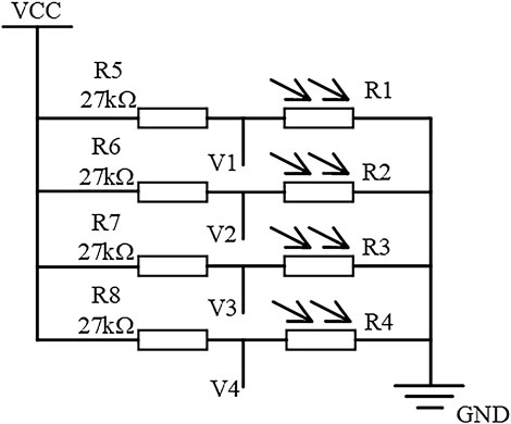
Figure 1. Control circuit diagram.
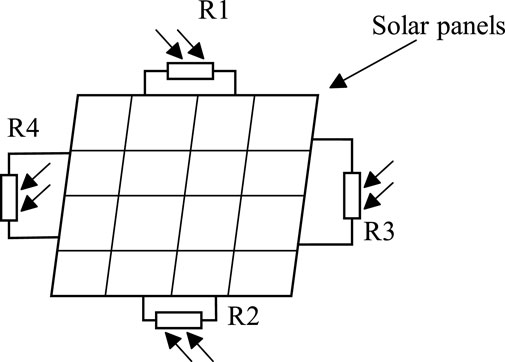
Figure 2. System architecture diagram.
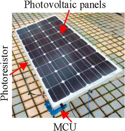
Figure 3. System architecture diagram.
The logic flowchart of the solar tracking algorithm, depicted in Figure 4, illustrates the process by which the system determines the sun’s position. It does so by analyzing the voltage output from the photovoltaic resistors. The system then adjusts the angle of the solar panel through MCU control, ensuring that it always faces the sun.
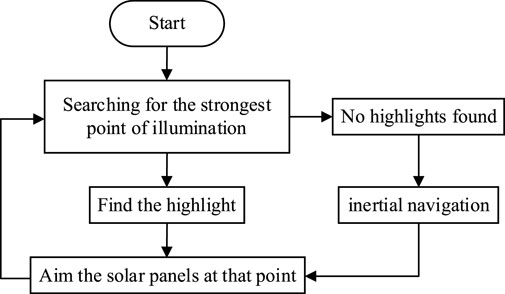
Figure 4. The logical flowchart of the sun tracking algorithm.
2.2 Cloud motion prediction model based on VGG
To enhance the prediction accuracy of cloud movement, our study integrated a camera onto the solar tracking device. We utilized the existing solar tracking mechanism to ensure that the camera’s field of view remained centered on the sun.
To improve cloud edge extraction, our study adopted a semantic segmentation and classification model based on Depthwise Separable Convolution Visual Geometry Group (DSCVGG). This approach overcomes the limitations of traditional edge detection algorithms, which often fail to accurately extract edge information from cloud images with uneven color levels.
The proposed model uses deep learning technology to input consecutive cloud images from two time periods. It automatically extracts cloud edge features and predicts the likelihood of cloud obscuration in the next time period through a classification mechanism. The design concept combines semantic segmentation of cloud images with cloud movement prediction, achieving integrated processing of edge extraction and motion prediction.
The VGG cloud prediction network employs the VGG19 model as its backbone, comprising 16 convolution layers, 3 fully connected layers, 5 pooling layers, and 2 deconvolution layers, as shown in Figure 5 (Huang et al., 2024). This network’s design draws inspiration from the VGG19 model, known for its hierarchical feature extraction capabilities in image recognition.
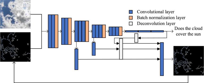
Figure 5. Structure diagrams of VGG model.
The VGG cloud prediction network takes the previous moment’s cloud edge image and the current cloud image as input. It outputs the current cloud edge image and predicts whether the sun will be obscured at the next moment. Its architecture is divided into nine main parts (Thakur et al., 2024). The first five parts consist of alternating 3 × 3 convolution layers and pooling layers, capturing local features. The use of smaller convolution kernels allows the network to increase depth without parameter inflation, enhancing expressiveness. Pooling layers reduce feature map resolution, preserving crucial information while decreasing computational complexity. The subsequent fully connected layers integrate local features into global features for image classification and prediction. The final deconvolution layers upsample feature maps, enabling precise cloud edge localization.
Through this hierarchical structure, the VGG cloud prediction network effectively learns image feature representations. It demonstrates exceptional performance in cloud edge extraction and sun obscuration prediction tasks (Wan et al., 2021). This network not only serves as an efficient auxiliary decision-making tool for solar tracking systems but also has significant application potential in renewable energy technology automation and weather forecasting accuracy improvement.
The convolution operation of the VGG19 network is represented as Eq. 1 in the following manner:
Where: yconv represents the output of the convolutional layer. f denotes the activation function.
2.3 VGG network based on depthwise separable convolutions
In order to reduce the computational time and model parameter count, this study has introduced a novel VGG model based on Depthwise Separable Convolution (DSC), referred to as DSCVGG. Depthwise Separable Convolution has been successfully applied in image classification tasks due to its capacity to significantly reduce the number of model parameters (Ayub and El-Alfy, 2024). Similar to the structure of the AlexNet network, DSC consists of two components: Depthwise Convolution (DC) and Pointwise Convolution (PC). A comparison between Depthwise Separable Convolution and standard convolution is illustrated in Figure 6.
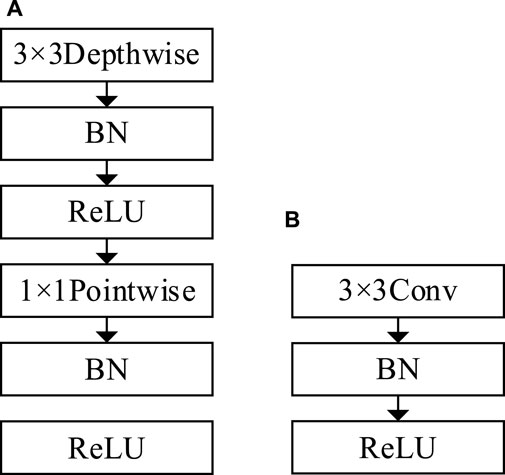
Figure 6. Comparison of DSC and normal convolution; (A) Depthwise Separable Convolution; (B) Normal Convolution.
In this research, one of the convolutional layers in the VGG network, located before the pooling layers, was replaced with Depthwise Separable Convolution, resulting in the creation of DSCVGG. The original VGG model contained a total of 14,591, 824, 384 parameters. Through the improved DSCVGG model, this parameter count has been reduced to 12,165, 165, 856, which is approximately 83.37% of the original model’s parameters. This substantial reduction effectively minimizes the parameter count of the VGG network.
This study utilized collected cloud data to train and fine-tune the DSCVGG network, successfully achieving accurate classification of current sky cloud patterns. By training on a vast dataset of cloud images, the DSCVGG network autonomously extracts crucial features from the images, distinguishing between various cloud types. This capability provides essential information for subsequent photovoltaic output predictions.
Overall, the introduction of the DSCVGG model, based on Depthwise Separable Convolution, offers improved computational efficiency and parameter reduction compared to the original VGG model. This novel model effectively classifies sky cloud patterns, which is valuable for enhancing the accuracy of photovoltaic output predictions.
3 Depthwise separable convolution Visual Geometry group-deep gate recurrent neural network
3.1 Deep neural network
A Deep Neural Network (DNN) is a multi-layer neural network that uses the error backpropagation algorithm for training. This algorithm allows the network to extract higher-level abstract features from raw data (Mittal, 2020). A DNN, as shown in Figure 7, comprises three main components, and the number of hidden layers can vary based on the application. A network with three or more hidden layers is considered deep or multi-layer (Miikkulainen et al., 2024).
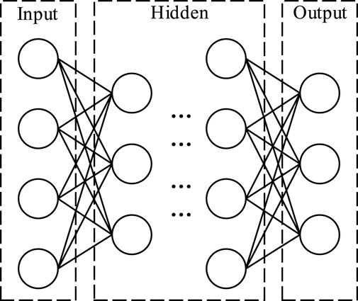
Figure 7. Deep neural network.
The training process of a DNN involves two primary steps: forward propagation and backward propagation. During forward propagation, sample data enters the network, passes through the hidden layers, and produces the network’s prediction output. The network’s prediction is then compared to the expected output, and any discrepancy results in error propagation. The network updates the weights and biases between layers continuously using optimization methods, aiming to make the prediction output match the expected output (Aldahdooh et al., 2022).
Through iterative training, DNNs can learn complex data relationships and patterns, demonstrating robust representation capabilities across various tasks. The error backpropagation algorithm enables self-correction and continuous performance improvement, making DNNs a cornerstone in modern machine learning and AI. They are pivotal in numerous applications and research domains.
3.2 Gate structure neural network
The Gate Recurrent Unit (GRU) is a recurrent neural network (RNN) unit used for sequence modeling. Its structure is illustrated in Figure 8 (Qin et al., 2024). Compared to Long Short-Term Memory (LSTM) units, GRU units have fewer parameters and lower computational costs, demonstrating excellent performance when handling long sequence data (Zhang et al., 2024). Its simplified architectural design and effective gate mechanisms enable it to better capture long-term dependencies within sequences, thereby enhancing the model’s performance on sequence data (Gozuoglu et al., 2024).
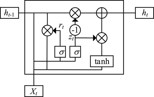
Figure 8. Structure diagram of gate recurrent unit.
The GRU unit consists of two gate mechanisms: the Reset Gate and the Update Gate. These gate mechanisms allow the GRU unit to control the flow and processing of information.
The forward propagation equation of GRU unit is shown in Eqs 2–5:
Where: rt represents the Reset Gate, zt represents the Update Gate, ht1 is the candidate hidden state, ht is the hidden state output, Wr and Ur are the weights for the Reset Gate, Wz and Uz are the weights for the Update Gate, W and U are the weights for the candidate hidden state, tanh is the hyperbolic tangent function,
Unlike LSTM units, GRU units have a single state variable, which reduces computational burden and memory requirements. They use the Reset Gate to integrate historical states and current inputs. Compared to LSTM, GRU has a simplified gate mechanism, making it more efficient at handling long-term dependencies in sequence modeling and reducing model complexity.
LSTM units have three gates: Forget Gate, Input Gate, and Output Gate, allowing them to capture and store information over longer time spans. In contrast, GRU simplifies the gate structure to include only the Update Gate and the Reset Gate. This simplification maintains model accuracy while enhancing training speed. With fewer gates, GRU units offer computational efficiency and excellent performance in handling sequence data.
3.3 Exponential linear unit activation function
Activation functions in neural networks are essential for introducing nonlinearity, which enhances the network’s ability to model complex relationships. However, traditional activation functions like Sigmoid and Tanh can encounter issues such as getting trapped in local optima with improper learning rate selection. Moreover, these functions can lead to the vanishing gradient problem, where the derivatives approach zero as signals propagate through multiple layers.
The Rectified Linear Unit (ReLU) activation function addresses some of these issues by outputting only non-negative values. This pushes activations towards positive values as the network depth increases, which can improve training speed. However, ReLU has a derivative of zero for negative inputs, which can lead to the “dying ReLU” problem, affecting training stability and accuracy.
To overcome these challenges, this paper utilizes the Exponential Linear Units (ELU) activation function, introduced by Clevert et al., in 2016. ELU maintains nonlinearity while providing a better handling of negative inputs, avoiding the “dying ReLU” problem (Clevert et al., 2016). This characteristic has made ELU popular in deep neural networks, particularly in natural language processing and image processing, where it has achieved notable results.
The mathematical expression for ELU, as shown in Eq. 6, offers the advantage of a linear response to positive inputs and a smooth treatment of negative inputs. This approach helps to improve network performance and addresses many of the issues associated with traditional activation functions (Kovaios et al., 2024).
Where: xin represents the input to the activation function. α controls the saturation of negative inputs. When α = 1, it becomes the ReLU activation function. In this paper, α is set to 0.01.
Figure 9 illustrates the four activation functions mentioned in the text.
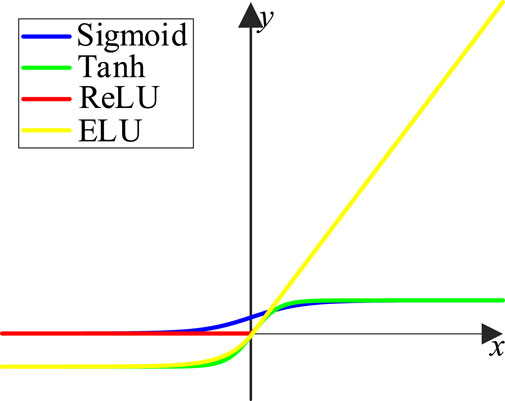
Figure 9. Diagram of Sigmoid, Tanh, ReLU and ELU activation functions.
3.4 Depthwise separable convolution Visual Geometry group-deep gate recurrent neural network
To effectively handle potential time series data, this paper proposes a Deep Gate Recurrent Neural Network (DGN). The DGN integrates concepts from Deep Neural Networks (DNN), GRU units, and the ELU activation function, as discussed in Section 3.1, Section 3.2, and Section 3.3. The network inputs include “time,” “temperature,” “humidity,” and “photovoltaic power output” at the current time step and predicts the “photovoltaic power output” at the next time step. Figure 10 depicts the overall structure of the network.
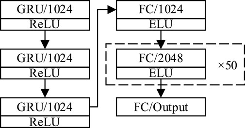
Figure 10. Structure diagram of Deep Gate Recurrent Neural Network.
The network begins with a three-layer stack of GRU units, which constructs a time series prediction network. This structure enables the network to model temporal dependencies in the input data. Following the GRU layers, the network transitions to a deep neural network consisting of 52 fully connected layers. These layers learn and produce the predicted photovoltaic power output. The fully connected layers comprise one layer with 1024 neurons, 50 layers with 2048 neurons each, and one output layer with a number of neurons equal to the desired output.
To mitigate the issue of vanishing gradients, which can degrade model accuracy, this paper replaces all ReLU activation functions following the fully connected layers with ELU activation functions. This replacement helps to maintain gradient flow and improve the network’s learning capabilities.
4 The short-term photovoltaic power output prediction model based on the DSCVGG-DGN
Existing short-term photovoltaic output prediction models have limitations in addressing the photovoltaic output fluctuations caused by cloud movement and obscuration. To address this issue, this paper proposes an integrated approach. By utilizing the output of the cloud movement prediction model based on DSCVGG to correct the output of the photovoltaic output prediction model based on the DGN network, a short-term photovoltaic output prediction model that can correct for the influence of cloud movement is constructed. This model effectively corrects the short-term photovoltaic output fluctuations caused by cloud movement and obscuration. The overall process is illustrated in Figure 11.
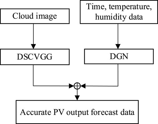
Figure 11. Structure diagram of photovoltaic short-term output prediction method based on the DSCVGG-DGN networ.
5 Photovoltaic power output prediction experiments and model performance evaluation
5.1 Hyperparameter tuning and data preprocessing
The experimental platform is based on a system equipped with an Intel Core i5-12400 central processing unit (CPU) and an Nvidia GeForce RTX 3060 graphics processing unit (GPU). All experiments were conducted using the PyTorch framework in the Python environment.
5.1.1 Hyperparameter configuration and data preprocessing for the cloud motion prediction model based on DSCVGG
The training dataset for cloud image data was derived from actual image captures. We took a photo every minute from 10:00 to 15:00 each day, resulting in a total of 2100 photographs of cloud movement. We used the cloud photos from the previous and current time intervals as model inputs, and the edge features of the clouds and whether the clouds obscured the sun in the next time interval as outputs to create the dataset for training the DSCVGG.
In this paper, the training epochs for the model are set to 300, and a cosine annealing learning rate is employed to dynamically adjust the learning rate during training, as expressed in Eq. 7. Compared to traditional fixed learning rates, the application of cosine annealing learning rate can help the model avoid getting stuck in local optima, making it more likely to reach a global optimum. The cosine annealing learning rate dynamically adjusts the learning rate during training. It starts with a relatively high learning rate at the beginning of training, which helps escape local optima, and gradually decreases the learning rate as training progresses, ensuring stable convergence when approaching the optimal solution. This strategy improves the performance, generalization capability, and convergence effectiveness of the model during neural network training (Loshchilov and Hutter, 2016).
Where: ηt is the current learning rate. ηmin is the minimum learning rate. ηmax is the maximum learning rate. Tcur is the current iteration number. Tmax is the maximum iteration number.
When the model’s training iterations reach Tmax, ηt resets to the maximum learning rate. This can cause sudden changes in the model’s accuracy and loss during training as it moves away from local optima but does not affect the final results.
The evaluation metrics include model accuracy (A) and the time required for the model to classify samples. The expression for accuracy is shown in Eq. 8.
Where: PTi represents correctly classified samples. PFi represents incorrectly classified samples.
5.1.2 Hyperparameter configuration and data preprocessing for the short-term photovoltaic power output prediction model based on DGN network
The photovoltaic power output data required for the power output prediction model is sourced from a photovoltaic power generation station within the Southern Power Grid, covering a 15-day period. The dataset includes the following key variables: “time,” “temperature,” “humidity,” and “photovoltaic power output.” In this model, the variables at the current time step are used as inputs, while the “photovoltaic power output” at the next time step serves as the output.
During the model training process, the cosine annealing learning rate is also employed to dynamically adjust the learning rate. The number of training epochs is set to 300. Two evaluation metrics are used in the experiments, namely, Mean Absolute Error (MAE) and Mean Squared Error (MSE), expressed mathematically as shown in Eqs 9, 10.
Where: EMA stands for Mean Absolute Error. EMS stands for Mean Squared Error. n represents the number of samples. yi represents the actual values.
5.2 Performance evaluation of cloud motion prediction model based on DSCVGG
To assess the efficacy of the cloud motion prediction model based on DSCVGG, a series of experiments were conducted on the collected cloud image dataset.
Firstly, to validate the performance of the DSCVGG model in cloud edge extraction, the experiment compared the edge extraction effects of three traditional edge detection algorithms—Roberts, Prewitt, and Sobel—against the DSCVGG model. The output results of these methods, as depicted in Figure 12, demonstrating the superior edge extraction capabilities of the DSCVGG model.
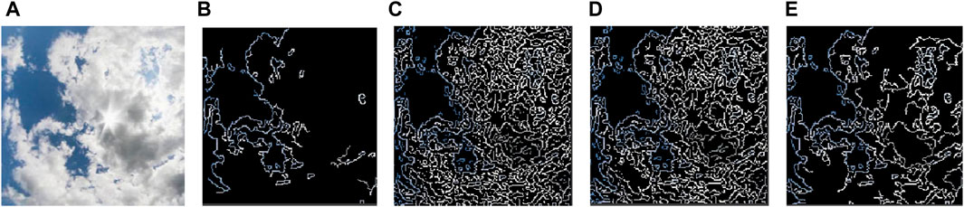
Figure 12. Cloud edge extraction results; (A) Original cloud map; (B) DSCVGG; (C) Roberts; (D) Prewitt (E) Sobel.
According to the results shown in Figure 12, it is evident that the DSCVGG model possesses a significant advantage in cloud edge extraction. The model effectively eliminates false edges caused by uneven cloud thickness, achieving high-precision edge extraction.
This performance enhancement is primarily attributed to the deep convolutional structure and strong feature learning capabilities of the DSCVGG model. By stacking multiple convolutional layers, the model can capture the complex textures and subtle changes in cloud images, thus more accurately defining the true edges of the clouds. This fine edge extraction is crucial for predicting cloud movement, as it directly impacts the adjustment precision of subsequent solar tracking systems and the efficiency of photovoltaic power generation.
Furthermore, to validate the accuracy of predictions regarding whether the clouds will obscure the sun at the next moment, we used the edge-extracted image from Figure 12B and the current cloud layer image as input, with the output being whether the clouds will obscure the sun at the next moment. As shown in Figure 13, during the experimentation, the DSCVGG model and the VGG model were trained and tested, and their performance was compared with other similar network models, such as NiNNet and ResNet. Figure 14 displays the accuracy of different models on the test set, while Table 1 provides a detailed breakdown of the accuracy of these four models in predicting whether the clouds will obscure the sun at the next moment. Table 2 records the average computation time required for these models to perform 1000 predictions.
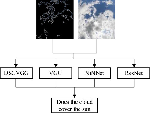
Figure 13. Input and output of the model.
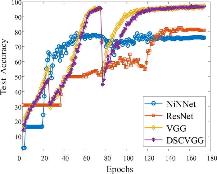
Figure 14. Test results of three models in cloud tier classification data.
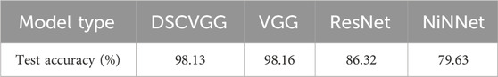
Table 1. Test accuracy for four models.
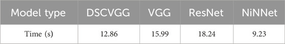
Table 2. Three models calculate the time required for 1000 times.
As indicated in Figure 14, the cloud motion prediction model based on DSCVGG converged after approximately 150 training iterations. When comparing the test accuracy as shown in Table 1, the DSCVGG model outperforms the NiNNet model and is slightly better than the deeper ResNet model, with its accuracy being comparable to that of the VGG model. Therefore, from an accuracy perspective, the DSCVGG model is exceptionally good.
Additionally, according to the data in Table 2, the DSCVGG model requires significantly less time to compute 1000 iterations compared to the VGG and ResNet models, but is slightly slower than the NiNVGG model. Considering the results from both Table 1 and Table 2, and taking into account both model performance and computational efficiency, we selected the validated DSCVGG model as the cloud motion prediction model to enhance the accuracy and stability of short-term photovoltaic output prediction.
5.3 Performance evaluation of short-term photovoltaic power output prediction model based on DGN network
To validate the effectiveness of the short-term photovoltaic power output prediction model based on the DGN network designed in this paper, experiments were conducted using the aforementioned photovoltaic power output data. Initially, the influence of the ELU activation function on the model’s loss was verified. In the experiment, the ReLU function following GRU was kept constant, and then the activation function following the fully connected layer was successively replaced with Sigmoid, Tanh, ReLU, and ELU functions. The model was trained and tested using the constructed dataset. The experimental results are shown in Figure 15 and Table 3.
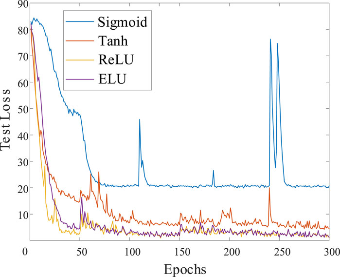
Figure 15. Test results for different activation function models.
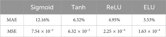
Table 3. Test MAE and MSE of model in different activation functions.
From the results shown in Figure 15 and Table 3, it can be observed that the DGN network based on the ELU activation function starts to converge around the 150th epoch, and its test loss, MAE, and MSE are lower than those of models using the other three activation functions. Therefore, for subsequent experiments, the DGN model based on the ELU activation function will be selected as the performance testing model.
To validate the effectiveness of the short-term photovoltaic power output prediction model based on the DGN network proposed in this paper, experiments were conducted using the aforementioned photovoltaic power output data. The experiments involved testing various models, including GRU, LSTM, RNN, and the DGN model proposed in this paper. The training and testing results of the experiments are shown in Figure 16 and Table 4.
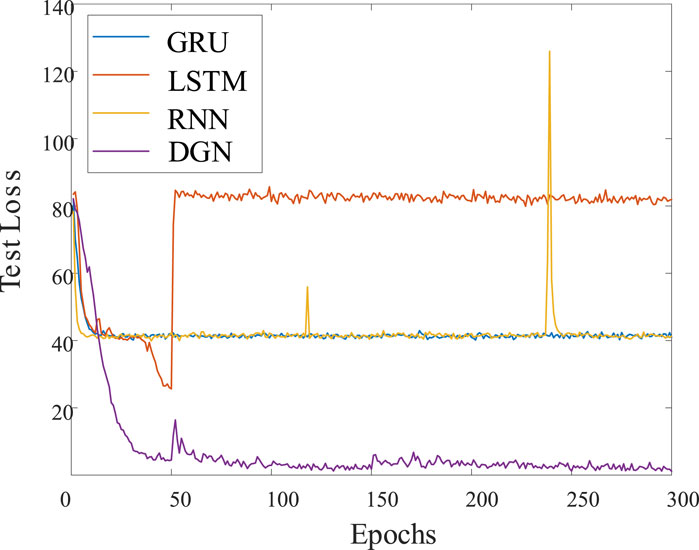
Figure 16. Photovoltaic output prediction test results of four models.
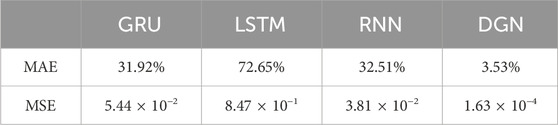
Table 4. Test MAE and MSE of four models.
Based on the experimental results from Figure 16 and Table 4, it can be observed that the convergence speed of the proposed DGN model, while slower than GRU, LSTM, and RNN models, starts to exhibit a lower test loss than the other three models after approximately 20 epochs. Beyond the 50th epoch, the DGN model’s test loss is significantly lower than that of the other three models. Additionally, the test MAE and MSE of the DGN model are much lower than those of the other three models. Therefore, for the subsequent fusion model, the DGN model is selected as the photovoltaic power output prediction model.
5.4 Evaluation of short-term photovoltaic power output prediction model based on DSCVGG-DGN network
To mitigate the short-term fluctuations in photovoltaic output caused by cloud movement and solar obscuration, this study integrates the cloud movement data predicted by the DSCVGG model with the input data of the DGN model described in Section 4.3, feeding them together into the DGN model. The aim is to enhance the accuracy of photovoltaic output predictions by incorporating information on cloud movement predictions. According to the research in literature (Ming et al., 2015), the influence coefficient of clouds on irradiance ranges from 0.4 to 0.9. In this experiment, we take the average influence coefficient of 0.65. This means that when the prediction indicates that clouds will obscure the sun, we consider that the photovoltaic output prediction data for the next moment needs to be multiplied by this influence coefficient to adjust the predicted value.
To verify the feasibility of the DSCVGG-DGN network model, this study compares its training results with the DGN model described in Section 4.3. Figure 17 presents the photovoltaic output prediction graphs for the four models, while Table 5 records the MSE and MAE of these models’ predictions. Since the LSTM model in Section 4 had a larger error, it was not included in the comparative experiment.
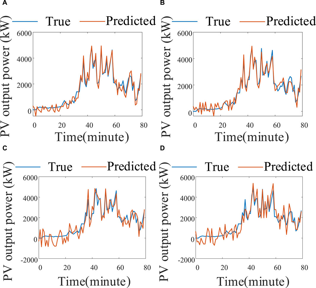
Figure 17. The DSCVGG-DGN model and the PV output prediction diagram of the other three models; (A) DSCVGG-DGN; (B) DGN; (C) RNN; (D) GRU.
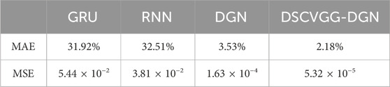
Table 5. The DSCVGG-DGN model was tested with three other models for MAE and MSE.
From Figure 17 and Table 5, it can be concluded that the short-term photovoltaic power output prediction model based on the DSCVGG-DGN network proposed in this paper achieves MAE and MSE values that meet the accuracy requirements for photovoltaic power output prediction. This model can accurately and quickly predict photovoltaic power output, effectively addressing the issue of DGN’s inability to predict short-term photovoltaic power fluctuations caused by cloud movement.
6 Conclusion and outlook
This paper proposed a short-term photovoltaic output prediction model based on the DSCVGG-DGN network. Through photovoltaic output prediction experiments and performance evaluation results, the following conclusions are drawn:
(1) The cloud motion prediction model proposed in this paper, based on DSCVGG, effectively reduces the number of model parameters and accelerates the calculation speed by replacing the previous convolution layer of the pooling layer with depthwise separable convolution. It can effectively extract cloud edge features, predict whether clouds will obscure the sun, and provide important information for subsequent photovoltaic output predictions.
(2) The photovoltaic output prediction model proposed in this paper, based on DGN, effectively improves the accuracy of model predictions by integrating GRU, ELU, and DNN networks, achieving high-precision predictions of photovoltaic output.
(3) The short-term photovoltaic output prediction model based on DSCVGG-DGN network constructed in this article effectively solves the problem of difficult prediction of photovoltaic output due to cloud cover by combining the cloud classification data of DSCVGG and the photovoltaic output prediction data of DGN, reducing the model’s MAE and MSE to 2.18% and 5.32 × 10⁻⁵, and achieving minute-level prediction of photovoltaic output.
In subsequent research, new short-term photovoltaic output prediction methods based on deep learning will be further developed to improve model accuracy. Our article did not further study the attenuation coefficient of photovoltaic output after cloud cover, and we hope to conduct more in-depth research on it in future work.
Data availability statement
The datasets presented in this article are not readily available because the data in this article is not convenient for public disclosure. Requests to access the datasets should be directed to WH, NjUxMjM3MjEyQHFxLmNvbQ==.
Author contributions
LZ: Writing–review and editing. SZ: Writing–review and editing. GZ: Writing–review and editing. LW: Writing–review and editing. BL: Writing–review and editing. ZN: Writing–review and editing. ZL: Writing–review and editing, Writing–original draft. ZY: Writing–original draft, Writing–review and editing. WH: Writing–original draft, Writing–review and editing.
Funding
The author(s) declare that financial support was received for the research, authorship, and/or publication of this article. This work was supported in part by the Yunnan Power Grid Corporation Science and Technology Project (YNKJXM20230124).
Conflict of interest
Authors LZ, GZ, and BL were employed by Yunnan Power Grid Co., Ltd., Qujing Power Supply Bureau. Authors SZ, LW, and ZN were employed by Yunnan Power Grid Corporation Planning and Construction Research Center.
The remaining authors declare that the research was conducted in the absence of any commercial or financial relationships that could be construed as a potential conflict of interest.
The funder had the following involvement in the study: project support, providing facilities, and partial funding for research activities. The funder did not influence the study design, data collection and analysis, decision to publish, or preparation of the manuscript.
Correction note
A correction has been made to this article. Details can be found at: 10.3389/fenrg.2025.1707498.
Publisher’s note
All claims expressed in this article are solely those of the authors and do not necessarily represent those of their affiliated organizations, or those of the publisher, the editors and the reviewers. Any product that may be evaluated in this article, or claim that may be made by its manufacturer, is not guaranteed or endorsed by the publisher.
References
Aldahdooh, A., Hamidouche, W., Fezza, S. A., and Déforges, O. (2022). Adversarial Example Detection for DNN Models: A Review and Experimental Comparison. Artificial Intell. Rev. 55 (6), 4403–4462. doi:10.1007/s10462-021-10125-w
Alharkan, H., Habib, S., and Islam, M. (2023). Solar Power Prediction Using Dual Stream CNN-LSTM Architecture. Sensors 23 (2), 945. doi:10.3390/s23020945
Ayub, M., and El-Alfy, E. S. M. (2024). MMNet-NILM: Multi-Target MobileNets for Non-Intrusive Load Monitoring. J. Intelligent Fuzzy Syst. (Preprint), 1–22. doi:10.3233/jifs-219426
Clevert, D.-A., Untertiner, T., and Hochreiter, S. (2016). Fast and accurate deep network learning by exponential linear units (ELUs). arXiv [Preprint]. doi:10.48550/arXiv.1511.07289
Fu, L., Yang, Y., Yao, X., Jiao, X., and Zhu, T. (2019). A regional Photovoltaic Output Prediction Method Based on Hierarchical Clustering and the mRMR Criterion. Energies 12 (20), 3817. doi:10.3390/en12203817
Gozuoglu, A., Ozgonenel, O., and Gezegin, C. (2024). CNN-LSTM Based Deep Learning Application on Jetson Nano: Estimating Electrical Energy Consumption for Future Smart Homes. Internet Things 26, 101148. doi:10.1016/j.iot.2024.101148
Huang, X., Peng, L., Mukherjee, S., Hamilton, C., Shi, X., Srinivasan, V., et al. (2024) “Fast VGG: An Advanced Pre-Trained Deep Learning Framework for Multi-Layered Composite NDE via Multifrequency Near-Field Microwave Imaging,” in Research in Nondestructive Evaluation, 1–17.
Kovaios, S., Pappas, C., Moralis-Pegios, M., Tsakyridis, A., Giamougiannis, G., Kirtas, M., et al. (2024). Programmable Tanh-and ELU-based Photonic Neurons in Optics-Informed Neural Networks. J. Light. Technol. 42, 3652–3660. doi:10.1109/jlt.2024.3366711
Loshchilov, I., and Hutter, F. 2016. “Sgdr: Stochastic Gradient Descent with Warm Restarts.” arXiv preprint arXiv:1608.03983.
Ma, T., Yang, H., and Lin, Lu (2020). Solar Photovoltaic System Modeling and Performance Prediction. Renew. Sustain. Energy Rev. 36, 304–315. doi:10.1016/j.rser.2014.04.057
Mellit, A., Massi Pavan, A., Ogliari, E., Leva, S., and Lughi, V. (2020). Advanced Methods for Photovoltaic Output Power Forecasting: A Review. Appl. Sci. 10 (2), 487. doi:10.3390/app10020487
Mellit, A., Pavan, A. M., and Lughi, V. (2021). Deep Learning Neural Networks for Short-Term Photovoltaic Power Forecasting. Renew. Energy 172, 276–288. doi:10.1016/j.renene.2021.02.166
Miikkulainen, R., Liang, J., Meyerson, E., Rawal, A., Fink, D., Francon, O., et al. (2024). “Evolving deep neural networks,” in Artificial intelligence in the age of neural networks and brain computing (Academic Press), 269–287.
Ming, D., Zhicheng, X., Bo, Z., and Rui, B. (2015). Solar Irradiance Model for Large-scale Photovoltaic Generation Considering Passing Cloud Shadow Effect. Proc. csee 35 (17), 4291–4299.
Mittal, S. (2020). A survey on Modeling and Improving Reliability of DNN Algorithms and Accelerators. J. Syst. Archit. 104, 101689. doi:10.1016/j.sysarc.2019.101689
Pierce, B. G., Stein, J. S., Braid, J. L., and Riley, D. (2022). Cloud Segmentation and Motion Tracking in Sky Images. IEEE J. Photovoltaics 12 (6), 1354–1360. doi:10.1109/jphotov.2022.3215890
Qin, Z., Yang, S., and Zhong, Y. (2024). Hierarchically Gated Recurrent Neural Network for Sequence Modeling. Adv. Neural Inf. Process. Syst. 36.
Son, Y., Zhang, X., Yoon, Y., Cho, J., and Choi, S. (2023). LSTM–GAN Based Cloud Movement Prediction in Satellite Images for PV Forecast. J. Ambient Intell. Humaniz. Comput. 14 (9), 12373–12386. doi:10.1007/s12652-022-04333-7
Sun, Y., Wang, F., Zhen, Z., Mi, Z., Liu, C., Wang, B., et al. (2015). “Research on short-term module temperature prediction model based on BP neural network for photovoltaic power forecasting,” in 2015 IEEE power & energy society general meeting (IEEE), 1–5.
Thakur, N., Bhattacharjee, E., Jain, R., Acharya, B., and Hu, Y. C. (2024). Deep Learning-Based Parking Occupancy Detection Framework Using ResNet and VGG-16. Multimedia Tools Appl. 83 (1), 1941–1964. doi:10.1007/s11042-023-15654-w
Wan, X., Zhang, X. U, and Liu, L. (2021). An improved VGG19 transfer learning strip steel surface defect recognition deep neural network based on few samples and imbalanced datasets. Appl. Sci. 11 (6), 2606. doi:10.3390/app11062606
Wang, K., Qi, X., and Liu, H. (2019). A comparison of Day-Ahead Photovoltaic Power Forecasting Models Based on Deep Learning Neural Network. Appl. Energy 251, 113315. doi:10.1016/j.apenergy.2019.113315
Wang, Y., Fu, W., Zhang, X., Zhen, Z., and Wang, F. (2023b). Dynamic Directed Graph Convolution Network Based ultra-short-term Forecasting Method of Distributed Photovoltaic Power to Enhance the Resilience and Flexibility of Distribution Network. IET Generation, Transm. Distribution 18, 337–352. doi:10.1049/gtd2.12963
Wang, Z., Wang, Y., Cao, S., Fan, S., Zhang, Y., and Liu, Y. (2023a). A Robust Spatial-Temporal Prediction Model for Photovoltaic Power Generation Based on Deep Learning. Comput. Electr. Eng. 110, 108784. doi:10.1016/j.compeleceng.2023.108784
Keywords: photovoltaic power output prediction, deep learning, depthwise separable convolution, VGG, gate recurrent neural network
Citation: Zhang L, Zhao S, Zhao G, Wang L, Liu B, Na Z, Liu Z, Yu Z and He W (2024) Short-time photovoltaic output prediction method based on depthwise separable convolution Visual Geometry group- deep gate recurrent neural network. Front. Energy Res. 12:1447116. doi: 10.3389/fenrg.2024.1447116
Received: 11 June 2024; Accepted: 15 July 2024;
Published: 01 August 2024; Corrected: 24 October 2025.
Edited by:
Sudhakar Babu Thanikanti, Chaitanya Bharathi Institute of Technology, IndiaReviewed by:
Vedran Mrzljak, University of Rijeka, CroatiaLing-Ling Li, Hebei University of Technology, China
Copyright © 2024 Zhang, Zhao, Zhao, Wang, Liu, Na, Liu, Yu and He. This is an open-access article distributed under the terms of the Creative Commons Attribution License (CC BY). The use, distribution or reproduction in other forums is permitted, provided the original author(s) and the copyright owner(s) are credited and that the original publication in this journal is cited, in accordance with accepted academic practice. No use, distribution or reproduction is permitted which does not comply with these terms.
*Correspondence: Zhijian Liu, MjQ4NDAwMjQ4QHFxLmNvbQ==