Non-intrusive residential load identification based on load feature matrix and CBAM-BiLSTM algorithm

With the increasing demand for the refined management of residential loads, the study of the non-invasive load monitoring (NILM) technologies has attracted much attention in recent years. This paper proposes a novel method of residential load identification based on load feature matrix and improved neural networks. Firstly, it constructs a unified scale bitmap format gray image consisted of multiple load feature matrix including: V-I characteristic curve, 1–16 harmonic currents, 1-cycle steady-state current waveform, maximum and minimum current values, active and reactive power. Secondly, it adopts a convolutional layer to extract image features and performs further feature extraction through a convolutional block attention module (CBAM). Thirdly, the feature matrix is converted and input to a bidirectional long short-term memory (BiLSTM) for training and identification. Furthermore, the identification results are optimized with dynamic time warping (DTW). The effectiveness of the proposed method is verified by the commonly used PLAID database.

1 Introduction

The informatization, automation, and intellectualization of smart grids are accelerating, resulting in increasing demands for transparency on the demand side of power systems. As a consequence, Non-Intrusive Load Monitoring (NILM) has become a burgeoning area of research.

In the realm of NILM technology, the interplay between load characteristics and identification algorithms assumes a pivotal role in shaping the ultimate identification outcome. The extraction of load characteristics indirectly governs the precision of the final NILM identification result. In reference (Sun et al., 2022), novel load characteristics emerge through the extraction of the gray and RGB elements from the V-I characteristic curve, and a comparative analysis of several lightweight Convolutional Neural Network (CNN) models ensues. Notably, this approach solely relies on the V-I characteristic curve, and encapsulates limited information. Reference (Feng et al., 2022) pioneers a method by fusing spatial features extracted by the CNN with temporal features extracted by the recursive neural network, presenting a novel avenue for creating load features. Nevertheless, the features generated pose challenges in their integration with diverse machine vision algorithms. Reference (Yin et al., 2023) provides empirical evidence supporting the notion that the amalgamation of multiple features significantly enhances the accuracy of algorithmic recognition. Reference (Kumar, 2024) and (Kumar et al., 2023a) extract the maximum power from the panel utilising MPPT (Maximum Power Point Tracking). Because using MTTP is oscillation in a steady-state condition, reference (Sukanya Satapathy and Kumar, 2020) proposes “Weight of Set Point Similarity” (WSPS) technique to obtain the maximum power point, and reference (Sukanya Satapathy and Kumar, 2019) proposes Modulated Perturb and Observe (MoPO) Maximum Power Point Tracking (MPPT) algorithm. To solve fixed step-change issues of classical “Perturb and Observe (P&O)” MPPT technique, reference (Kumar et al., 2023b) introduces a novel “Single-input Adaptive Fuzzy-Logic (SIAFL)” tuned P&O MPPT algorithm.

In response to the aforementioned challenges, this article proposes a unified grayscale image in a bitmap format, incorporating multiple load feature matrices, including the V-I characteristic curve, 1–16 harmonic currents, 1-cycle steady-state current waveform, maximum and minimum current values, active and reactive power. This grayscale image comprehensively encapsulates the characteristic information of each dimension of the load and allows for further expansion as needed.

The accuracy of NILM identification results is directly influenced by the choice of the identification algorithm. To solve the unit commitment (UC) problem, reference (Kumar et al., 2016) adopted a new hybrid method of “Gaussian Harmony Search” (GHS) and “Jumping Gene Transfer” (JGT) algorithm (GHS-JGT). Reference (Kumar et al., 2022) used human psychological optimization to track the global maximum power point. References (Liu et al., 2022) leverage Dynamic Time Warping (DTW) to mitigate the overlearning phenomenon in deep learning algorithms, thereby enhancing identification accuracy. Reference (Liu et al.) adopts a Bidirectional Long Short-Term Memory (BiLSTM) network to implement a probabilistic sparse attention mechanism for identifying multi-state processes of devices. In summary, this article presents a non-invasive load recognition algorithm that combines the CBAM-BiLSTM neural network with DTW. This algorithm effectively extracts pertinent information from images, filters out extraneous data, mitigates overfitting in certain samples by the neural network, and enhances the overall accuracy of load recognition.

Traditional CNN are limited to extracting coarse feature matrices from images. To enhance the extraction of detailed features related to load characteristics, the CBAM is employed to further refine the extraction process. This paper introduces a non-intrusive residential electrical monitoring method based on an enhanced neural network model incorporating CBAM. The method consists of the following steps: 1) Extraction of a grayscale image representing the load feature matrix; 2) Extraction of image features through convolutional layers; 3) Further feature refinement using the Channel Attention Module (CAM) and Spatial Attention Module (SAM); 4) Training and identification using a BiLSTM neural network; 5) Optimization of identification results using the DTW algorithm. The key advantage of this algorithm lies in its ability to effectively extract relevant load features through CAM and SAM, discard irrelevant information, ultimately leading to a significant improvement in load identification accuracy.

2 Improved neural network load identification algorithm flow based on attention mechanism

Based on the Enhanced Neural Network with CBAM, this paper introduces a non-intrusive load identification algorithm, integrating CBAM-BiLSTM and DTW. Figure 1 illustrates the algorithm’s flowchart, comprising the following steps:1) Collect voltage and current data from household appliances, extracting features such as V-I characteristic curve, current fundamental wave, 2–16th harmonic currents, one-cycle steady-state current waveform, maximum and minimum current values during steady-state operation, active power, and reactive power. Normalize the data and convert it into a standardized grayscale image in Bitmap (BMP) format. 2) Employ a convolutional layer for image feature extraction, transforming the image into a preliminary feature matrix. 3) Conduct additional feature extraction using CBAM, refining the coarse feature matrix of each electrical appliance into a detailed load feature matrix. 4) Train and identify the load using a BiLSTM neural network. The fine feature matrix is processed through a fully connected layer and input to the BiLSTM network, yielding the identification result P_BiLSTM (Probability vector obtained from CBAM BiLSTM neural network) = {p₁, p₂, … , p_n}, where p_n represents the probability that an unknown load is identified as a known load. 5) Optimize identification results using the DTW algorithm. Compare the similarity between DTW and the feature vector in the load database to obtain the identification result P_DTW (Probability vector obtained by using the DTW optimization algorithm.) = {p₁, p₂, … , p_n}, where p_n represents the probability that an unknown load is identified as a known load. Combine P_BiLSTM and P_DTW to derive the final identification result.

Figure 1

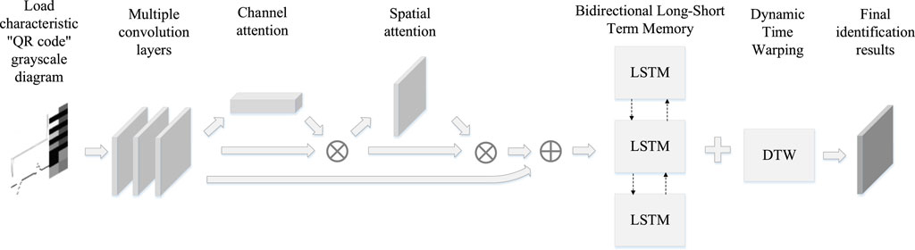
Figure 1. Flow chart of the improved load identification algorithm based on attention mechanism.

3 Construction of grayscale map of the load feature matrix

This paper utilizes the publicly available Plug-Level Appliance Identification Dataset (PLAID) (Medico et al., 2020) for simulation verification. PLAID gathers current and voltage data from various appliances, extracting key features such as the V-I characteristic curve, current fundamental wave, 2–16th harmonic currents, one cycle of the current steady-state waveform, current maximum and minimum values, active power, and reactive power. To transform this data into grayscale images representing the load feature matrix, a normalization process is initially applied, followed by permutation and combination techniques to construct the load grayscale image.

3.1 Data normalization

To commence, normalization is applied to the seven types of feature data. The specific steps are outlined as follows.

3.1.1 V-I characteristic curve

Starting from the same time point, the steady-state waveform of one cycle of current and voltage is considered. One cycle is set to be represented by k data points, and the current and voltage data are then normalized to a uniform scale of 0–1 through a normalization process. The formula for this normalization is as follows in Equations 1, 2:

${i_i}^{*}=\left[\frac{I_i-\min I}{\max I-\min I}\right],i=1,2,\cdots ,k(1)$

$u_i^{*}=\left[\frac{U_i-\min U}{\max U-\min U}\right],i=1,2,\cdots ,k(2)$

where, i_i ^* (u_i^*) represents the data of the i-th sampling point of the normalized current (voltage); I_i (U_i) represents the data of the i-th sampling point of the original current; minI (minU) represents the minimum value of the original current (voltage) in one cycle; maxI (maxU) represents the maximum value of the original current (voltage) in one cycle; [ ] denotes a rounding operation.

Drawing the grayscale image of the V-I characteristic curve involves using voltage as the abscissa and current as the ordinate. This image can be viewed as a k * k matrix, where the elements’ values range from 0 to 1.

3.1.2 1–16th harmonic currents

The current data is decomposed into the current fundamental wave I₁ and the 2–16th harmonic current I_h through Fourier series transformation, and the harmonic current is normalized with the current fundamental wave I₁ as the reference value, as follows in Equation 3.

$I_{\mathrm{h}}^{*}=\frac{I_h}{I_1},h=2,3,\dots ,16(3)$

where, I_h^* is the per-unit value of I_h after normalization with I₁ as the reference value.

3.1.3 One-cycle current steady-state waveform

Suppose a current cycle is represented by k data points (k is taken as 64 in this article), where the maximum current value is maxI and the minimum value is minI. At each k/m point, a data point is taken and converted into an m × n matrix. It is then normalized, as shown in Equation 4.

$I_i^{*}=\frac{I_i-\min I}{\max I-\min I}*n,i=1,2,\cdots ,\frac{k}{m}(4)$

where, I_i ^* is the per-unit value of the i-th current data point after normalization; I_i represents the data of the i-th sampling point of the original current.

3.1.4 Current maximum and current minimum

The maximum current and the minimum current are normalized, as shown in Equations 5, 6.

$\max I^{*}=\frac{\max I-{\mathrm{I}}_{\min }}{{\mathrm{I}}_{\max }-{\mathrm{I}}_{\min }}(5)$

$\min I^{*}=\frac{\min I-{\mathrm{I}}_{\min }}{{\mathrm{I}}_{\max }-{\mathrm{I}}_{\min }}(6)$

Where, maxI^* (minI^*) represents the normalized per-unit value of the maximum (minimum) current value. I_max (I_min) represents the reference value of the maximum (minimum) current in normalization. The current of a typical household load is usually between −20A and 20A. Therefore, this article takes I_max for 20A, and I_min is equal to −20A.

3.1.5 Active and reactive power

The active and reactive power are normalized, as shown in Equations 7, 8.

$P^{*}=\frac{P}{{\mathrm{P}}_{\max }}(7)$

$Q^{*}=\frac{Q-{\mathrm{Q}}_{\min }}{{\mathrm{Q}}_{\max }-{\mathrm{Q}}_{\min }}(8)$

where, P^*(Q^*) is the per-unit value of the normalized active (reactive) power. P_max represents the reference value of the maximum active power in normalization. Q_max (Q_min) represents the reference value of the maximum (minimum) reactive power in normalization. After testing various household appliances, this article found that the active power of ordinary household loads usually does not exceed 2,500 W, and the reactive power is usually between −200 var and 150 var. Therefore, in this article, P_max is taken as 2,500 W, Q_max is taken as 150 var, and Q_min is taken as −250 var.

3.2 Draw the load grayscale image

After normalization, the seven types of feature data are all converted into data in the range of 0 to 1, but their data sizes are different, and they need to be combined to form a grayscale image of a uniform size. According to the different specifications of the data used by scholars, data formats of different sizes will eventually be formed. In this paper, the format of the V-I characteristic curve is a two-dimensional matrix of 48 × 48, and the format of the steady-state current waveform is 48 × 24. The two-dimensional matrix of the current fundamental wave and the 2–16th harmonic currents is a one-dimensional vector of 1 × 16, and the format of the current maximum value, current minimum value, active power, and reactive power is a one-dimensional vector of 1 × 4.

To arrange and combine the seven types of characteristic data. 1) Generate an empty matrix of size 72 × 72. 2) Fill the V-I characteristic curve into the element range of the empty matrix (1:48, 1:48). 3) Fill the steady-state current waveform into the empty matrix (49:72, 1:48). 4) Fill the current fundamental wave and the 2–16th harmonic currents into the element range (1:48, 49:72), with each feature occupying a range of 6 × 12 elements. 5) Fill the current maximum value, current minimum value, active power, and reactive power into (49:72, 49:72), where each feature occupies a 12 × 12 element range.

A schematic diagram of the process is shown in Figure 2. Using MATLAB, a feature matrix consisting of seven types of feature data is converted into a uniformly scaled BMP format load feature grayscale image, and a 72 × 72 matrix is output on the computer. The range of matrix elements is from 0 to 255, representing 256 gray levels in the image.

Figure 2

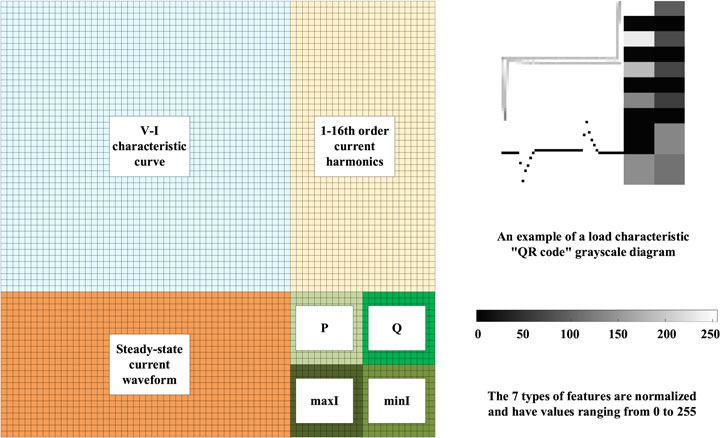
Figure 2. Schematic diagram of the construction of the grayscale image of the load feature matrix.

4 Convolutional block attention module to extract refined features

The fine feature matrix is further extracted through CBAM (Woo et al., 2018). The CBAM includes both a CAM and a SAM, in which the activation function is sigmoid, and the dimension of the extracted fine feature matrix is 72 × 72 × 20.

Figure 3 is the flow chart of fine feature matrix extraction by CBAM. First, a rough feature matrix is extracted from the two-dimensional code gray image of the load feature through a multi-layer convolution layer, and then a fine feature matrix is extracted by CBAM. It is noted that CBAM includes two independent sub-modules: the CAM and the SAM, which respectively focus on the attention mechanism on the channel and space, and then couple the feature data.

A. Multi-layer Convolutional Layers to Extract Coarse Feature Matrix

Figure 3

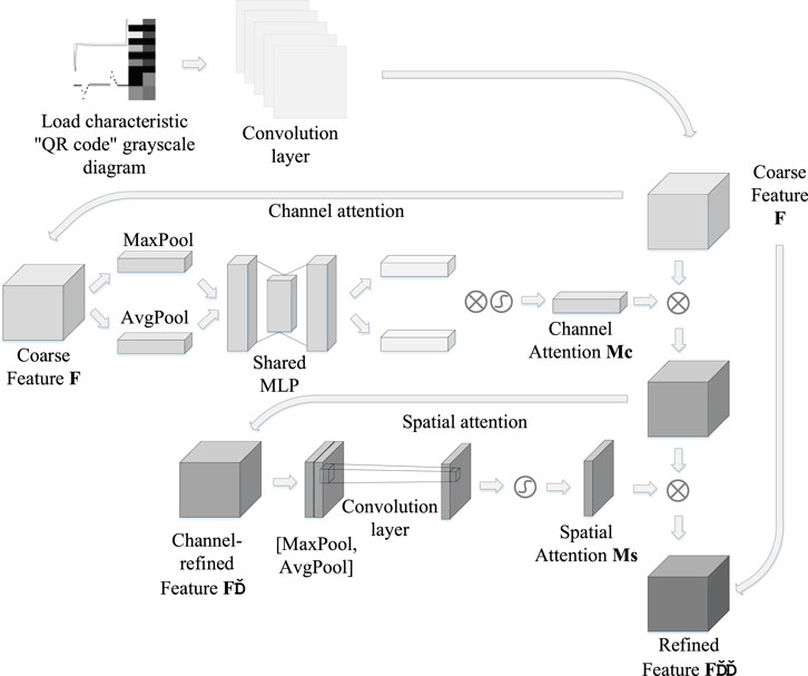
Figure 3. The flow chart of the convolution block attention mechanism module extracting fine feature matrix.

The grayscale image of the load feature matrix is input into the CNN, and the rough feature matrix of each electrical appliance is extracted. The structure of the CNN is as follows: 1) An input layer with dimensions 72 × 72 × 1. 2) A convolution layer with dimensions72 × 72 × 20, and the kernel function with dimensions 5 × 5 (20). 3) The activation function of the CNN is sigmoid.

The grayscale image of the load feature matrix is processed by the CNN to obtain a rough feature matrix of size 72 × 72 × 20.

B. Channel Attention Module (CAM) Computation

Figure 4 shows the schematic diagram of the CAM.

Figure 4

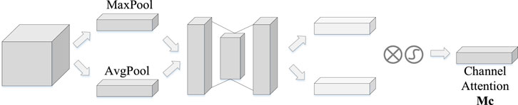
Figure 4. Schematic diagram of the CAM.

The specific calculation process of the CAM is as follows in Equation 9:

$\begin{array}{l}{F}^{\prime }=\text{sigmoid}\left(\text{MLP}\left(\text{avgpool}\left(F\right)\right)+\text{MLP}\left(\text{maxpool}\left(F\right)\right)\right)\\ =\text{sigmoid}\left(w^1{w}^2{F}_{avg}^{C\times 1\times 1}+w^1{w}^2{F}_{\max }^{C\times 1\times 1}\right)\end{array}(9)$

where, F′ represents the channel attention output feature matrix; F represents the rough feature matrix; sigmoid is the activation function; MLP represents the multi-layer perceptron; maxpool (avgpool) represents the maximum (average) pooling layer; w¹ and w² represent the weight of the MLP; F_max^{C × 1 × 1} (F_avg^{C × 1 × 1}) represents the one-dimensional vector after the maximum (average) pooling operation.

C. Spatial Attention Module (SAM) Computation

Figure 5 shows the schematic diagram of the SAM.

Figure 5

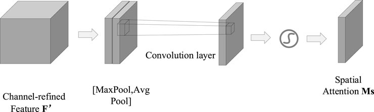
Figure 5. Schematic diagram of the SAM.

The formula for calculating spatial attention is in Equation 10:

$F^{″}=\text{sigmoid}\left(\text{convd}\left(\text{avgpool}\left(F^{\prime }\right)\right);\text{convd}\left(\text{maxpool}\left(F^{\prime }\right)\right)\right)(10)$

where, F″ represents the fine feature matrix; F′ represents the channel attention output feature matrix; sigmoid represents the activation function; convd represents the convolution operation; avgpool (maxpool) represents the average (maximum) pooling operation.

D. Results Coupled Calculation

Figure 6 is the schematic diagram of the CBAM. It is noted that the CBAM contains two independent sub-modules, namely the CAM and the SAM. The attention mechanism transforms and subsequently couples the feature data.

Figure 6

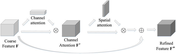
Figure 6. Schematic diagram of result coupling.

The process is shown in the following Equations 11, 12:

$F^{\prime }=F\otimes M_C(11)$

$F^{″}=F\oplus \left(F^{\prime }\otimes M_s\right)(12)$

where, F′ represents the output feature matrix of channel attention; F represents the rough feature matrix; Mc represents the output of the CAM; M_s represents the output of the SAM, represents the corresponding multiplication of each element. F″ represents the CBAM output feature matrix, represents the corresponding addition of elements in the two matrices.

E. Convolutional Block Attention Module (CBAM) Extracts Refined Feature Matrix

Figure 7 shows a schematic diagram of the feature extraction of the grayscale image by the SAM. The upper row of black background pictures in the figure is the grayscale image of the V-I characteristic curve, and its values are distributed from 0 to 1, with 0 representing pure black, and 1 representing pure white. The lower row is the weight extraction of the grayscale image by the SAM, the spatial attention output two-dimensional weight matrix M_s, whose matrix elements are distributed from 0 to 1, representing the weight by which the pixel should be multiplied. The larger the weight, the higher the information importance of the pixel.

Figure 7

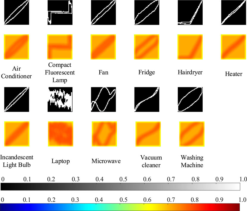
Figure 7. Schematic diagram of spatial attention module (SAM) extracting refined feature matrix from a grayscale image.

As observed in the figure, for pixels containing characteristic information in the grayscale image, CBAM increases the weight value by multiplication. Pixels with less information correspond to smaller weight values. Similarly, in channel attention, a larger weight is multiplied for a layer with more information content, and a smaller weight is multiplied for a layer with less information content. Finally, a fine feature matrix with more useful information is obtained.

5 Bidirectional long short-term memory neural network training and identification

5.1 Principle of bidirectional long short-term memory (BiLSTM) artificial neural network

Long short-term memory (LSTM) (Karim et al., 2018) is an improved recurrent neural network (RNN). It is mainly aimed at solving the problem of gradient vanishing during RNN training process. It exhibits robust performance when dealing with sequential data. LSTM and its variants have found extensive applications in the NILM problem in recent years (Kaselimi et al., 2020; Le et al., 2021).

LSTM is composed of multiple identical cell structures. Each cell structure includes three essential components: Forget gate, Input gate, Output gate.

The cell structure topology is illustrated in Figure 8:

Figure 8

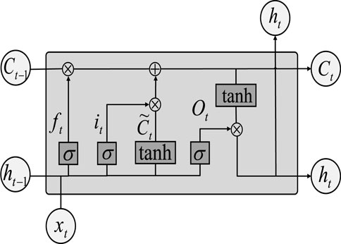
Figure 8. The LSTM algorithm structure.

In Figure 8, C_t represents the cell state information at time t, h_t represents the cell output information at time t, and x_t represents the cell input information at time t. f_t represents the output of the forget gate at time t, and its operation can be expressed by the Equation 13:

$f_t=\sigma \left(w_{\text{FG}}\cdot \left[h_{t-1},x_t\right]+b_{\text{FG}}\right)(13)$

where, σ is the sigmoid activation function, w_FG and b_FG represent the weight and bias of the forget gate, respectively, [h_t-1, x_t] represents the combination of the input at time t and the output at the previous time.

i_t and ${\stackrel{\sim }{C}}_t$ together represent the output of the input gate, and their operations can be represented by Equations 14, 15:

$i_t=\sigma \left(w_{\mathrm{i}}\cdot \left[h_{t-1},x_t\right]+b_{\mathrm{i}}\right)(14)$

${\stackrel{\sim }{C}}_t=\tanh \left(w_{\mathrm{c}}\cdot \left[h_{t-1},x_t\right]+b_{\mathrm{c}}\right)(15)$

where, σ and tanh represent the activation function, w_i and w_c represent the weight, and b_i and b_c represent the bias.

The operation of the cell state update can be expressed by Equation 16:

$C_t=f_t\cdot C_{t-1}+i_t\cdot {\stackrel{\sim }{C}}_t(16)$

where, C_t (C_t-1) represents the cell state information at time t (t-1), f_t represents the output of the forget gate at time t, i_t and ${\stackrel{\sim }{C}}_t$ together represent the output of the input gate.

The operation of the final output gate can be expressed by Equations 17, 18:

$O_t=\sigma \left(W_{\text{OG}}\left[h_{t-1},x_t\right]+b_{\text{OG}}\right)(17)$

$h_t=O_t\cdot \tanh \left(C_t\right)(18)$

where, O_t represents the intermediate information of the output gate, h_t (C_t) represents the cell output (state) information at time t, σ and tanh represent the activation function, W_OG represents the weight, and b_OG represents the bias.

The BiLSTM algorithm is a variant algorithm of LSTM. It consists of one layer of LSTM for forward propagation and another layer of LSTM for backward propagation. The forward layer initiates the input iteration from the starting point of the sequence, and the reverse layer starts the input iteration from the end of the sequence (Xie et al., 2022). Finally, the output results of the two layers are concatenated to obtain the identification result. Its network structure is illustrated in Figure 9:

Figure 9

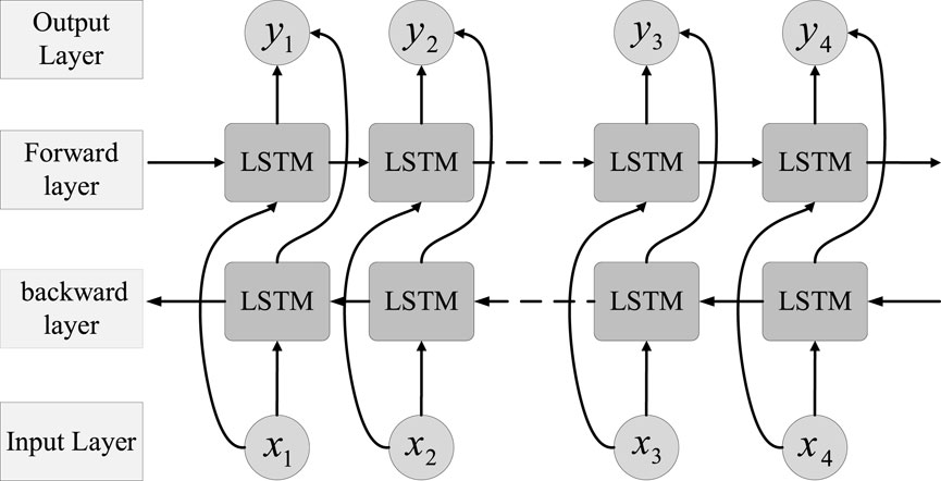
Figure 9. The structure of the BiLSTM algorithm.

The BiLSTM algorithm can be expressed by the following Equations 19–21:

$h_t=f\left(W_1{x}_t+W_2{h}_{t-1}\right)(19)$

$r_t=f\left(W_3{x}_t+W_5{r}_{t+1}\right)(20)$

$y_t=g\left(W_4{h}_t+W_6{r}_t\right)(21)$

where, x_t represents the input at time t; h_t and r_t represent the output of the forward layer and reverse layer at time (t), respectively; y_t represents the output of the output layer at time t; f represents the activation function of the forward layer and reverse layer; g represents the activation function of the output layer; W₁ and W₃ are the weight matrices of the input layer mapped to the forward layer and the reverse layer; W₂ and W₅ are the weight matrices of the forward layer and the reverse layer from the previous calculation moment mapped to the current calculation moment; W₄ and W₆ are the weight matrices that map the output of the forward layer and the reverse layer to the output layer.

5.2 Neural network training parameters

We convert the fine feature matrix F″ of each electrical appliance into a one-dimensional feature vector through a 1 × 1 × 100-dimensional fully connected layer. This vector is then input into the BiLSTM neural network model for learning. In the final identification step, the unknown load undergoes the same Steps 1 to 3, and the processed data is input into the trained neural network for identification, yielding the final identification result. The load is identified by training the BiLSTM neural network.The structure of the BiLSTM neural network is as follows: 1) A fully connected layer with a dimension of (1, 100). 2) A BiLSTM layer with a layer dimension of (1, 100), where the activation functions are sigmoid and tanh. 3) A fully connected layer with a dimension of (1, 11). 4) A classification layer with a dimension of (1, 11), where the activation function is Softmax.

During the training process, the following settings are applied: 1) Gradient threshold: 1. 2) Training period: 100,857 iterations per cycle. 3) Learning rate: 0.001. 4) The training process utilizes the adaptive moment estimation optimization algorithm.

Inputting the unknown load results in the identification output, which takes the form of 11 values. Each value, ranging between 0 and 1, represents the probability that the load consists of one of the 11 kinds of electrical appliances.

6 Dynamic time warping programming optimization identification algorithm

6.1 Principles of dynamic time warping (DTW)

The DTW algorithm, commonly utilized in speech recognition, operates on the principle of dynamic programming. It calculates the most matching part of two time series, breaking down the process of finding an optimal solution into an optimal path that automatically identifies a local optimal solution. Unlike the Euclidean distance, the DTW algorithm excels in accurately measuring similarity for locally scaled and locally drifted curves. In practice, DTW is often coupled with CNN (Chen et al., 2022) for identification purposes (Afrasiabi et al., 2020; Trelinski and Kwolek, 2021).

In Figures 10, 11 the amplitude, phase, and frequency of the two current signals for Load 1 and Load 2 are different. Through some deformation and displacement processing, the coincidence rate of the two signals is improved.

Figure 10

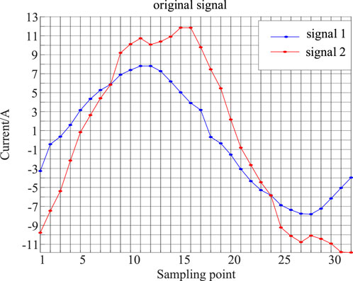
Figure 10. The original signal of load 1 and load two.

Figure 11

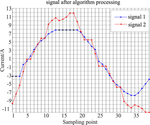
Figure 11. The signal of load 1 and load 2 after dynamic time warping (DTW) processing.

Here’s an explanation of how to find similarities between two different signals. In Figure 12, there are two signals, A and B. The DTW algorithm finds the optimal path by calculating the local best matching point of the A signal corresponding to the B signal and computing the distance between them.

Figure 12

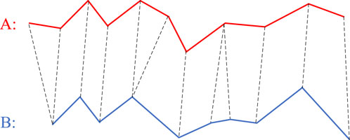
Figure 12. DTW optimal point matching.

Figure 13 is a schematic diagram of the DTW algorithm illustrating the process of finding the optimal path. The algorithm involves the following steps: 1) Calculate the Euclidean distances for each point in Signal 1 and Signal 2, forming a matrix of distances. 2) Identify two diagonal axes in this matrix. 3) Find a special path between points along these diagonals, where the sum of each element should be the smallest among all possible paths.

Figure 13

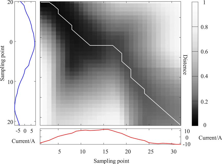
Figure 13. Schematic diagram of DTW finding the optimal path.

The mathematical model of the DTW algorithm is summarized as follows: There are two time-series signals A = {a₁, a₂, … , a_n} and B = {b₁, b₂, … , b_m}. First calculate the cost matrix D between A and B, which is an n × m-order matrix. Its expression is shown in Equation 22:

$D=\left[\begin{array}{cccc}{d}_{11}& d_{12}& \cdots & d_{1m}\\ d_{21}& d_{22}& \cdots & d_{2m}\\ ⋮& ⋮& \ddots & ⋮\\ d_{n1}& d_{n2}& \cdots & d_{nm}\end{array}\right](22)$

Where, d_nm represents the Euclidean distance between a_n and b_m, where d_nm = ||a_n-b_m||²; ||·||² represents the 2-norm.

Then, we find the optimal path from d₁₁ to d_nm in the cost matrix, minimize the sum of d on the path, and construct a new cost matrix D_dist, where the element dist_ij is shown in Equation 23:

$D=\left[\begin{array}{cccc}{d}_{11}& d_{12}& \cdots & d_{1m}\\ d_{21}& d_{22}& \cdots & d_{2m}\\ ⋮& ⋮& \ddots & ⋮\\ d_{n1}& d_{n2}& \cdots & d_{nm}\end{array}\right](23)$

where, the weighted sum of the shortest local cost measures between A and B is the value of the element distnm of the cost matrix D_dist.

6.2 Coupling of identification results

Since the identification mechanisms of the BiLSTM neural network and DTW algorithm are quite distinct, especially for electrical appliances with high identification degrees, combining the results from both algorithms can effectively enhance the final identification accuracy. The final probability vector P_final, is formed by combining the results of the two algorithms using the following Equation 24:

$P_{\text{final}}\left(i\right)=\left\{\begin{array}{c}{P}_{\text{BiLSTM}}\left(i\right),P_{\text{DTW}}\left(i\right)<P_{\text{BiLSTM}}\left(i\right)\\ P_{\text{DTW}}\left(i\right),P_{\text{DTW}}\left(i\right)\ge P_{\text{BiLSTM}}\left(i\right)\end{array}\right.(24)$

where, i represents the number of elements, ranging from 1 to k; P_final(i) represents the final probability value of the i-th test sample; P_BiLSTM(i) represents the i-th test sample identified by the CBAM-BiLSTM network. The probability value of P_DTW(i) represents the probability value of the i-th test sample identified by the DTW algorithm.

The elements P_BiLSTM(i) and P_DTW(i) in Equation 24 are the largest in the load identification vectors P_BiLSTM = {p₁,p₂, … ,p_n} and P_DTW = {p₁,p₂, … ,p_n} respectively. They represent the probability that the target appliance i is identified as a certain appliance by the two algorithms, and their calculation formulas are as follows in Equations 25, 26:

$P_{\text{BiLSTM}}\left(i\right)=\text{Softmax}\left(W_4\left(h_i\right)+W_6\left(r_i\right)\right)(25)$

$P_{\text{DTW}}\left(i\right)=\frac{{\displaystyle \sum _{k=1}^n}dist\left(k\right)-dist\left(i\right)}{{\displaystyle \sum _{k=1}^n}dist\left(k\right)}(26)$

In the formulas: i represents the recognized electrical appliance; Softmax represents the activation function; W₄ represents the weight matrix from the output of the BiLSTM forward layer to the output layer; W₆ represents the weight matrix from the output of the BiLSTM reverse layer to the output layer; h_i represents the forward layer of the output neuron corresponding to the i-th electrical appliance; r_i represents the output of the output neuron corresponding to the i-th electrical appliance in the reverse layer; dist(k) represents the calculated DTW between the target sample and the k-th electrical appliance feature distance. The smaller the distance, the more similar the target sample is to the appliance.

7 Simulation analysis

To verify the practicality of the algorithm, relevant simulation experiments were designed for verification. In this study, 11 electrical appliances from PLAID, including air conditioners, energy-saving lamps, electric fans, refrigerators, hair dryers, electric heaters, incandescent lamps, laptop computers, microwave ovens, vacuum cleaners, and washing machines, were selected as experimental appliances. A robust algorithm should exhibit good generalization performance (Rafiq et al., 2021; Schirmer and Mporas, 2022). 100 sets of randomly selected data from each category of electrical appliances were chosen as the test set, with the remaining collected data serving as the training set.

7.1 Comparison of V-I characteristic curve and the load feature matrix

Figure 14 displays the recognition results using the common V-I feature curve as the feature matrix, while Figure 15 shows the recognition results using the grayscale image as the feature matrix. The recognition algorithm employed is the CBAM-BiLSTM algorithm. The results are presented in the form of a confusion matrix commonly used in deep learning (Salmana et al., 2022). Confusion matrix is commonly used for performance evaluation of supervised learning algorithms, which can intuitively reflect the comparison between real labels and predicted labels.

Figure 14

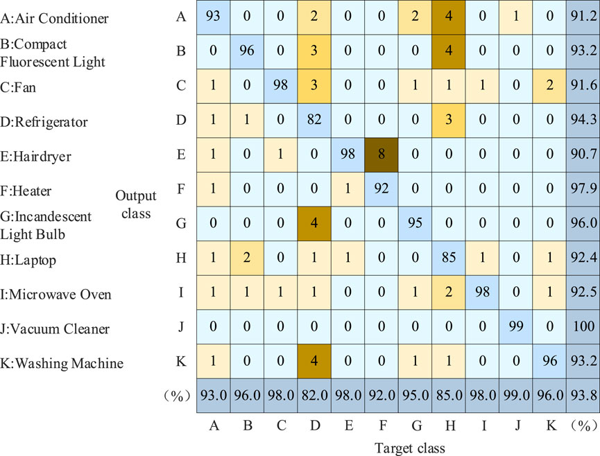
Figure 14. Identification result when V-I characteristic curve is used as load identification feature.

Figure 15

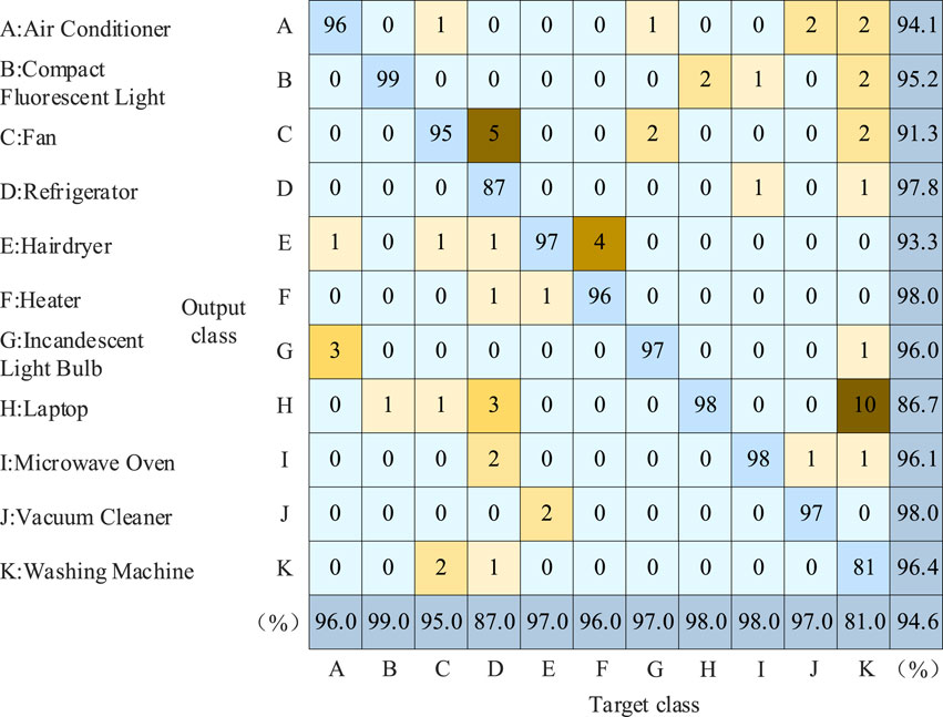
Figure 15. The identification result when the grayscale image is used as the load identification feature.

The vertical axis of the confusion matrix represents the predicted electrical appliances, while the horizontal axis represents the actual electrical appliances. In this study, 11 electrical appliances were selected as experimental appliances. Therefore, the elements range (1:11, 1:11) of the confusion matrix are recognition results. For example, in Figure 15, the value “96” in the first row and first column indicates that 96 air conditioning samples were identified as such; the value “1” in the first column of the fifth row represents that 1 air conditioning sample were identified as hair dryers. The elements range (12, 1:11) of the confusion matrix represent recall of electrical appliances. The elements range (1:11, 12) of the confusion matrix represent precision of electrical appliances. The elements range (12, 12) of the confusion matrix represents the overall accuracy.

The overall accuracy, precision and recall of electrical appliances can be calculated through the confusion matrix, and the formula is as follows in Equations 27–29:

$E=\frac{{\displaystyle \sum _{i=1}^{11}}\left(T_i+R_i\right)}{N}(27)$

$H_i=\frac{T_i}{T_i+Q_i},i=1,2,\dots ,11(28)$

$G_i=\frac{T_i}{T_i+F_i},i=1,2,\dots ,11(29)$

where, i represents the i-th electrical appliance, a total of 11 electrical appliances; E represents the overall accuracy; G_i (H_i) represents the precision (recall) of electrical appliance i; N represents the actual total number of electrical samples; R_i (T_i) represents that the real category of the electrical appliance i is negative (positive), and the model recognizes it as negative (positive); Q_i (F_i) represents that the real category of the electrical appliance i is positive (negative), but the model recognizes it as negative (positive).

When the V-I characteristic curve is used as a load recognition feature, the overall recognition accuracy through Equation 27 is 93.8%. When the grayscale image is used as the load recognition feature, the overall recognition accuracy through Equation 27 is 94.6%.

By comparative analysis, the new load identification features are not universally applicable to all electrical appliances. For example, in the identification of washing machines, compared to using the V-I characteristic curve to identify four errors, the grayscale image did not recognize 19 samples as washing machines. However, except for individual appliances, the new load characteristics can improve the recognition accuracy of appliances to varying degrees. For example, in laptop recognition, compared to the V-I characteristic curve, the grayscale image corrected the recognition results of 13 samples. Overall, the grayscale images exhibit better recognition performance.

7.2 Comparison: Before and after adding convolutional block attention module (CBAM)

Figures 16, 17 present the identification results of 11 electrical appliances before and after the addition of CBAM, showcased in the form of a confusion matrix. The objective is to assess whether adding CBAM to CNN can enhance recognition accuracy and reduce false detection rates.

Figure 16

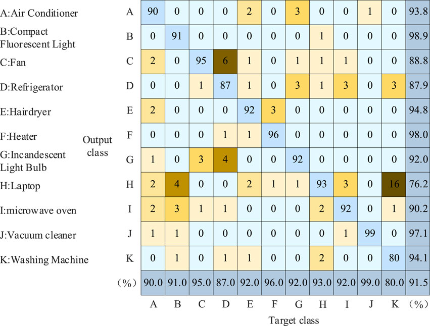
Figure 16. Algorithm identification results before the CBAM is added.

Figure 17

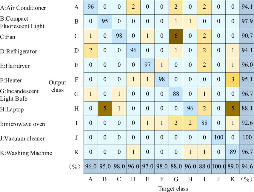
Figure 17. Algorithm identification results after the CBAM is added.

Before the addition of CBAM, the overall identification accuracy through Equation 27 is 91.5%. After the addition of CBAM, the overall identification accuracy through Equation 27 increases to 94.6%.

By comparative analysis, The CBAM module proves to be beneficial for improving the overall identification effect of the algorithm. For example, in the identification of refrigerators, before CBAM addition, six samples were mistakenly identified as electric fans. After the CBAM module, by further extracting fine features, rectifies this misclassification. What’s more, in the identification of washing machines, before CBAM addition, 16 samples were misclassified as laptop computers. After CBAM incorporation, this number is reduced to 5 cases. Therefore, the addition of CBAM contributes to the improved accuracy of load identification.

7.3 Comparison before and after dynamic time warping (DTW) optimization algorithm

Figures 14–17 present the load recognition results without the utilization of the DTW optimization algorithm, while Figure 18 illustrates the recognition outcomes after incorporating the DTW-optimized neural network algorithm. Figure 17 shows that the maximum accuracy is 94.6% before adding DTW optimization algorithm. According to Figure 18, after adding DTW optimization algorithm, the overall recognition accuracy through Equation 27 experiences a notable improvement, reaching 96.9%.

Figure 18

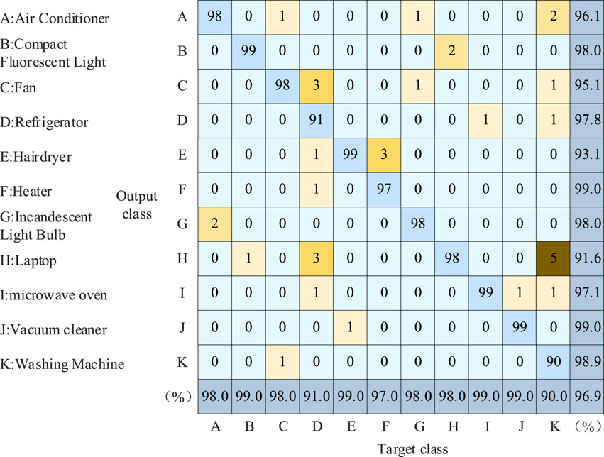
Figure 18. Identification results after DTW optimization algorithm.

Through comparative analysis, the beneficial complementary effect of DTW on the error recognition of neural networks becomes apparent, leading to an effective enhancement in the recognition accuracy for most electrical appliance types. For example, in the identification of incandescent lamps, before adding DTW optimization algorithm, six samples were mistakenly identified as electric fans. After adding DTW optimization algorithm, only one sample was mistakenly identified as an electric fan.

Therefore, DTW serves as a valuable complement, addressing errors in neural network recognition and significantly improving accuracy. Optimizing the CNN-BiLSTM network through DTW proves to be an effective strategy for enhancing the overall recognition accuracy of the algorithm.

8 Conclusion and outlook

This paper introduces a Non-Intrusive Residential Load Identification Algorithm incorporating an Attention Mechanism. The introduction of grayscale images solves the problem of low identification accuracy in traditional V-I characteristic curve. Adding CBAM can extract a fine feature matrix from feature matrix transformations. The fine feature matrix improves the overall recognition accuracy of the algorithm. After coupling with DTW algorithm optimization, the recognition accuracy can be further improved.

This paper is research on NILM technology based on event detection. By default, the total load curve is decomposed into several unknown loads, and there is still room to improve the load decomposition accuracy in practical applications. In the next step, we can study the total load curve decomposition method, or directly identify the load combination without decomposing the load (Schirmer and Mporas, 2023).

Data availability statement

The raw data supporting the conclusions of this article will be made available by the authors, without undue reservation.

Author contributions

SL: Conceptualization, Formal Analysis, Methodology, Writing–original draft. BZ: Project administration, Software, Validation, Writing–original draft. YZ: Data curation, Supervision, Validation, Writing–original draft. JY: Formal Analysis, Validation, Investigation, Writing–review and editing. XB: Supervision, Visualization, Writing–review and editing. DL: Funding acquisition, Visualization, Writing–review and editing.

Funding

The author(s) declare that financial support was received for the research, authorship, and/or publication of this article. This work was supported in part by the National Natural Science Foundation of China (51977127), and the Shanghai Talent Development Fund (2018004).

Conflict of interest

Author YZ was employed by State Grid Zhejiang Shaoxing Electric Power Co., Ltd. Author JY was employed State Grid Shandong Electric Power Company Ultra-High Voltage Company.

The remaining authors declare that the research was conducted in the absence of any commercial or financial relationships that could be construed as a potential conflict of interest.

Publisher’s note

All claims expressed in this article are solely those of the authors and do not necessarily represent those of their affiliated organizations, or those of the publisher, the editors and the reviewers. Any product that may be evaluated in this article, or claim that may be made by its manufacturer, is not guaranteed or endorsed by the publisher.

References

Afrasiabi, M., khotanlou, H., and Mansoorizadeh, M. (2020). DTW-CNN: time series-based human interaction prediction in videos using CNN-extracted features. Vis. Comput. 36 (6), 1127–1139. doi:10.1007/s00371-019-01722-6

CrossRef Full Text | Google Scholar

Chen, J., Wang, X., Zhang, X., and Zhang, W. (2022). Temporal and spectral feature learning with two-stream convolutional neural networks for appliance recognition in NILM. IEEE Trans. Smart Grid 13 (1), 762–772. doi:10.1109/TSG.2021.3112341

CrossRef Full Text | Google Scholar

Feng, J., Li, K., Zhang, H., Zhang, X., and Yao, Y. (2022). Multi-channel spatio-temporal feature fusion method for NILM. IEEE Trans. Industrial Inf. 18 (12), 8735–8744. doi:10.1109/tii.2022.3148297

CrossRef Full Text | Google Scholar

Karim, F., Majumdar, S., Darabi, H., and Chen, S. (2018). LSTM fully convolutional networks for time series classification. IEEE Access 6, 1662–1669. doi:10.1109/access.2017.2779939

CrossRef Full Text | Google Scholar

Kaselimi, M., Doulamis, N., Voulodimos, A., Protopapadakis, E., and Doulamis, A. (2020). Context aware energy disaggregation using adaptive bidirectional LSTM models. IEEE Trans. Smart Grid 11 (4), 3054–3067. doi:10.1109/tsg.2020.2974347

CrossRef Full Text | Google Scholar

Kumar, N. (2024). EV charging adapter to operate with isolated pillar top solar panels in remote locations. IEEE Trans. Energy Convers. 39 (1), 29–36. doi:10.1109/tec.2023.3298817

CrossRef Full Text | Google Scholar

Kumar, N., Panigrahi, B. K., and Singh, B. (2016). A solution to the ramp rate and prohibited operating zone constrained unit commitment by GHS-JGT evolutionary algorithm. Int. J. Electr. Power and Energy Syst. 81, 193–203. doi:10.1016/j.ijepes.2016.02.024

CrossRef Full Text | Google Scholar

Kumar, N., Saxena, V., Singh, B., and Ketan Panigrahi, B. (2022). Intuitive control technique for grid connected partially shaded solar PV-based distributed generating system. IET Renew. Power Gener. 14 (4), 600–607. doi:10.1049/iet-rpg.2018.6034

CrossRef Full Text | Google Scholar

Kumar, N., Saxena, V., Singh, B., and Panigrahi, B. K. (2023b). Power quality improved grid-interfaced PV assisted onboard EV charging infrastructure for smart households consumers. IEEE Trans. Consumer Electron. 69 (4), 1091–1100. doi:10.1109/tce.2023.3296480

CrossRef Full Text | Google Scholar

Kumar, N., Singh, H. K., and Niwareeba, R. (2023a). Adaptive control technique for portable solar powered EV charging adapter to operate in remote location. IEEE Open J. Circuits Syst. 4, 115–125. doi:10.1109/ojcas.2023.3247573

CrossRef Full Text | Google Scholar

Le, T.-T.-H., Heo, S., and Kim, H. (2021). Toward load identification bas ed on the hilbert transform and sequence to sequence long short-term memory. IEEE Trans. Smart Grid 12 (4), 3252–3264. doi:10.1109/tsg.2021.3066570

CrossRef Full Text | Google Scholar

Liu, Y., Qiu, J., Lu, J., Wang, W., and Ma, J. (2022). A single-to-multi network for latency-free non-intrusive load monitoring. IEEE Trans. Netw. Sci. Eng. 9 (2), 755–768. doi:10.1109/tnse.2021.3132309

CrossRef Full Text | Google Scholar

Liu, Z., Zhang, L., Zhang, L., and Tianyao, Ji. Wavelet decomposition-bi-directional long-short term memory neural network with prob-sparse attention for non-intrusive load monitoring. CSEE J. Power Energy Syst. doi:10.17775/CSEEJPES.2022.04570

CrossRef Full Text | Google Scholar

Medico, R., De Baets, L., Gao, J., Giri, S., Kara, E., Dhaene, T., et al. (2020). A voltage and current measurement dataset for plug load appliance identification in households. Sci. Data 7 (1), 49–4463. doi:10.1038/s41597-020-0389-7

PubMed Abstract | CrossRef Full Text | Google Scholar

Rafiq, H., Shi, X., Zhang, H., Li, H., Ochani, M. K., and Shah, A. A. (2021). Generalizability improvement of deep learning-based non-intrusive load monitoring system using data augmentation. IEEE Trans. Smart Grid 12 (4), 3265–3277. doi:10.1109/tsg.2021.3082622

CrossRef Full Text | Google Scholar

Salmana, A., Shahab, A., Usma, H., Kamranb, J., Jalee, R., and Sajida, A. (2022). Confusion matrix-based modularity induction into pretrained CNN. Multimedia Tools Appl., 1380–7501. doi:10.1007/s11042-022-12331-2

CrossRef Full Text | Google Scholar

Schirmer, P. A., and Mporas, I. (2022). Device and time invariant features for transferable non-intrusive load monitoring. IEEE Open Access J. Power Energy 9, 121–130. doi:10.1109/oajpe.2022.3172747

CrossRef Full Text | Google Scholar

Schirmer, P. A., and Mporas, I. (2023). Non-intrusive load monitoring: a review. IEEE Trans. Smart Grid 14 (1), 769–784. doi:10.1109/tsg.2022.3189598

CrossRef Full Text | Google Scholar

Sukanya Satapathy, S., and Kumar, N. (2019) “Modulated Perturb and Observe maximum power point tracking algorithm for solar PV energy conversion system,” in 2019 3rd international conference on recent developments in control, automation and power engineering (RDCAPE).

CrossRef Full Text | Google Scholar

Sukanya Satapathy, S., and Kumar, N. (2020). Framework of maximum power point tracking for solar PV panel using WSPS technique. IET Renew. Power Gener. 14 (10), 1668–1676. doi:10.1049/iet-rpg.2019.1132

CrossRef Full Text | Google Scholar

Sun, M. Y., Yang, B. K., Zheng, Z., Nie, Y. H., Cui, W. P., Liu, R., et al. (2022). “Comparative research between several lightweight CNN models for non-intrusive load monitoring using transfer learning approach,” in 2022 international conference on big data, information and computer network (China: Sanya), 189–195.

CrossRef Full Text | Google Scholar

Trelinski, J., and Kwolek, B. (2021). CNN-based and DTW features for human activity recognition on depth maps. Neural Comput. and Applic 33, 14551–14563. doi:10.1007/s00521-021-06097-1

CrossRef Full Text | Google Scholar

Woo, S., Park, J., Lee, J. Y., and Kweon, I. S. (2018). CBAM: convolutional block attention module. Lect. Notes Comput. Sci. Incl. Subser. Lect. Notes Artif. Intell. Lect. Notes Bioinforma. 11211, 3–19. doi:10.1007/978-3-030-01234-2_1

CrossRef Full Text | Google Scholar

Xie, J., Shi, W., and Shi, Y. (2022). Research on fault diagnosis of six-phase propulsion motor drive inverter for marine electric propulsion system based on res-BiLSTM. Machines 10 (9), 736. doi:10.3390/machines10090736

CrossRef Full Text | Google Scholar

Yin, H., Zhou, K., and Yang, S. (2023). Non-intrusive load monitoring by load trajectory and multi feature based on DCNN. IEEE Trans. Industrial Inf. 19 (10), 10388–10400. doi:10.1109/tii.2023.3240924

CrossRef Full Text | Google Scholar