Top oil temperature prediction at a multiple time scale for power transformers based on adaptive extended Kalman filter

To achieve load management optimization and timely failure warning for power transformers, as well as improve the reliability of the power network, this paper proposes a multiple time scale prediction method for top oil temperature (TOT) based on an adaptive extended Kalman filter (AEKF) algorithm. This method combines the Kalman filter (KF) algorithm and the D. Susa thermal model. The TOT, oil exponent and oil time constant are taken as state variables, while the ambient temperature and load current are used as input variables. The iterative optimization of the oil exponent and oil time constant is realized by comparing the estimated and observed TOT values. Moreover, the proposed method utilizes an adaptive noise estimator to correct the noise statistics parameters, which simplifies the initial noise setting and thus further improves the TOT prediction accuracy. A case study is conducted with two 110 kV transformers. The results show that comparing the thermal equivalent circuit model and the extended KF algorithm, the proposed method has a higher accuracy in the intraday ultra-short-term prediction on a 15-min time scale and day-ahead short-term prediction on a 24-h time scale for the TOT.

1 Introduction

The top oil temperature (TOT) is an important indicator for evaluating the thermal characteristics of a power transformer. Accurate prediction of changes in the TOT is of vital practical significance for timely assessing the transformer’s load capacity and detecting the potential thermal faults (Lachman et al., 2003; Shiravand et al., 2021; Liu et al., 2022). The TOT is related to the structure, size, cooling mode, etc. of the transformer and varies with the changes in the external environmental parameters and load operation conditions (Wang et al., 2019; Zhang et al., 2024). Depending on the prediction time cycle, the TOT predictions are divided into day-ahead short-term predictions with a day as the time cycle, and intraday ultra-short-term predictions with an hour or a minute as the time cycle. For short-term/ultra-short-term predictions at multiple time scales for the TOT, the existing methods mainly include the empirical thermal model calculation method given in the IEEE and IEC guidelines and the thermal equivalent circuit method, as well as the prediction method based on artificial intelligence (AI) algorithms (He et al., 2000; Chen et al., 2009).

In the (IEEE Std C57.91, 2011; IEC 60076-7, 2017) guidelines, a differential equation is used to describe the rise of the TOT relative to the ambient temperature. In the thermal equivalent circuit method, the most common model is the dynamic thermal model proposed by D. Susa (Susa et al., 2005a; Susa et al., 2005b; Sönmez and Komurgoz, 2018). This model considers the non-linear thermal resistance caused by the changes in oil viscosity with temperature. Therefore, it can predict the changes in the TOT more accurately compared with IEEE and IEC thermal models. In terms of the above three dynamic thermal models, the key parameters that affect the prediction performance include the rated TOT rise Δθ_oil,r, the ratio of the rated load loss to the no-load loss R, the oil exponent n and the rated oil time constant τ_oil,r. Among them, the accurate values of Δθ_oil,r and R can be obtained through the factory test, while the values of τ_oil,r and n are usually difficult to determine. Generally, the latter two parameters are roughly assessed according to the transformer’s capacity and cooling type. The fixed values obtained through the rough assessment cannot accurately reflect information such as the transformer’s existing performance and degree of oil aging, thus affecting the accuracy of the TOT prediction.

In addition to the above dynamic thermal models, many scholars use the support vector regression (SVR) model and artificial neural networks to predict the TOT (Wang K. et al., 2020). In (Tan et al., 2022), a TOT prediction method based on the SVR algorithm is proposed. The correlation coefficients of nine variables such as temperature, humidity, and light intensity with the TOT are calculated, and the main variables among them are selected as the input vectors. In (Li et al., 2021), the authors establish an improved weighted SVR model for the TOT prediction and use a particle swarm optimization algorithm to optimize the hyperparameters of the SVR model. The TOT prediction model using a long short-term memory (LSTM) network is proposed in (Dong et al., 2023), with the ambient temperature, and the active and reactive power of the load data as the characteristic parameters. The above methods realize TOT prediction using AI algorithms while considering multiple parameters such as ambient temperature, humidity, and load factor as input variables. It is necessary to estimate multiple parameters at the same time. If there is a large deviation in the prediction of a parameter, the TOT prediction accuracy will be greatly reduced. The cumulative effect of the deviation is more significant, especially in the prediction at a long-time scale. In addition, machine learning-based prediction methods require a large amount of historical measurement data during the training, and the measured data inevitably contains measurement noise. If the noise component cannot be effectively identified and filtered out in the training process, it will also affect the TOT prediction effect.

The Kalman filter (KF) algorithm is capable of iteratively optimizing the parameters by calculating the deviation between the estimated data and the observed data, which can control the deviation within a certain range and avoid the effect of error accumulation under the prediction at a long-time scale (Chen and Su, 2013; Lai et al., 2017; Alvarez et al., 2019). Therefore, this paper combines the KF algorithm and the D. Susa thermal model and proposes an adaptive extended Kalman filter (AEKF) based TOT prediction method. This method uses the Taylor Series expansion method to realize the linearization transformation of the nonlinear equations of the D. Susa thermal model. The oil exponent and the oil time constant are optimized iteratively by comparing the deviation of the estimated and measured TOT values. As a result, the TOT prediction accuracy is improved under both the intraday ultra-short-term and day-ahead short-term prediction. Moreover, the proposed model considers an adaptive noise estimator to realize the adaptive estimation of the statistical covariates of the TOT observation noise, thus improving the robustness of the model and the adaptability to uncertain environments. Two 110 kV transformer entities are analyzed. The results show that the proposed method outperforms the traditional dynamic thermal model in multiple time scale prediction with 15 min or 24 h as a period, and has a better adaptability to the measurement noise.

2 Extended Kalman filter algorithm

Kalman filter is an algorithm that uses the linear system state equation and the observation data of the system for the optimal estimation of the system state. The KF combines the dynamic information of the target with the observation results to suppress the impact of noise for a more accurate estimate of the target position. This estimation can be a filter or smooth for the current and past target positions, or it can also be the prediction for future positions. However, the KF is only applicable to linear system state equations. For the TOT prediction, which involves a non-linear system, it is necessary to introduce Extended Kalman filter (EKF) algorithm. The basic idea of the EKF algorithm is to linearize the nonlinear system using the Taylor Series expansion, and then perform subsequent calculations using the KF framework.

2.1 Establishment of prediction model

First, the derivation of the prediction model of the EKF is introduced. The Taylor Series expansion is a method of using the n-degree polynomial about (x-x₀) to approach the function value f(x) with n-order derivatives at x = x_0. When the variable is a multi-dimensional vector, the one-dimensional Taylor Series expansion is shown as Equation 1:

$f\left(\mathit{x}\right)=f\left({\mathit{x}}_0\right)+{\left[\nabla f\left({\mathit{x}}_0\right)\right]}^{\mathrm{{\rm T}}}\left(\mathit{x}-{\mathit{x}}_0\right)+o^n(1)$

where ${\left[\nabla f\left({\mathit{x}}_0\right)\right]}^T=\mathit{J}\left({\mathit{x}}_0\right)$ denotes the Jacobian matrix and oⁿ denotes the high-order infinitesimal. In practical engineering applications, the EKF can satisfy the computational accuracy requirements by taking only the first-order derivative in the Taylor Series expansion of nonlinear functions.

For a nonlinear state equation, the state migration equation and observation equation of the EKF system are as follows Equations 2, 3:

${\mathit{x}}_k=\mathit{f}\left({\mathit{x}}_{k-1}\right)+{\mathit{s}}_k(2)$

${\mathit{z}}_k=\mathit{h}\left({\mathit{x}}_{k-1}\right)+{\mathit{v}}_k(3)$

where the state migration function f indicates the mapping relationship of the state vector before and after a specific time, the measurement function h indicates the mapping relationship between the state vector and the measured value. x_k is the real state vector at time k, s_k is the state migration noise vector. z_k and v_k are the observation vector and the observation noise vector, respectively. Generally, both s_k and v_k follow a Gaussian distribution with the average value being zero vector. Their covariance matrices are Q and R_k, respectively.

With the Taylor Series expansion, the state migration Equation 2 changes to Equation 4:

${\mathit{x}}_k=\mathit{f}\left(〈x_{k-1}〉\right)+{\mathit{F}}_{k-1}\left({\mathit{x}}_{k-1}-〈{\mathit{x}}_{k-1}〉\right)+{\mathit{s}}_k(4)$

where <x_k-1> is the estimated value of the state vector at the previous time k-1. F_k-1 is the Jacobian matrix of the function f(x) at the estimated previous time <x_k-1>.

Next, the covariance matrix ${\mathit{\Sigma }}_k^{\prime }$ between the real value x_k and the predicted value ${\mathit{x}}_k^{\prime }$ is calculated using the state migration Equation 4:

$\begin{array}{l}{\mathit{\Sigma }}_k^{\prime }=〈{\mathit{e}}_k^{\prime }{\mathit{e}}_k^{\prime T}〉=\langle \left({\mathit{x}}_k-{\mathit{x}}_k^{\prime }\right){\left({\mathit{x}}_k-{\mathit{x}}_k^{\prime }\right)}^T\rangle \\ \begin{array}{cc}& =\end{array}{\mathit{F}}_{k-1}\langle \left({\mathit{x}}_{k-1}-〈{\mathit{x}}_{k-1}〉\right)\cdot {\left({\mathit{x}}_{k-1}-〈{\mathit{x}}_{k-1}〉\right)}^T\rangle {\mathit{F}}_{k-1}^T+\langle {\mathit{s}}_k{\mathit{s}}_k^T\rangle \\ \begin{array}{cc}& =\end{array}{\mathit{F}}_{k-1}{\mathit{\Sigma }}_{k-1}{\mathit{F}}_{k-1}^T+\mathit{Q}\end{array}(5)$

In Equation 5, x_k, <x_k> and the state migration noise vector s_k are independent of each other, and the multiplicative covariance is 0. <s_ks_k^T> is the covariance matrix of the state migration noise, expressed in Q.

2.2 Establishment of updated correction model

Next, the derivation process of the updated correction model of the EKF is introduced. Since the observation vector in the TOT prediction is the TOT, it is regarded as a linear mapping and then the observation equation is expressed as (Equation 6):

${\mathit{z}}_k={\mathit{H}}_k{\mathit{x}}_k+{\mathit{v}}_k(6)$

where H_k is the observation matrix and v_k is the observation noise vector. Therefore, the transition functions of the prediction state vector to the observation vector are as follows (Equations 7, 8):

${\mathit{\mu }}_0={\mathit{H}}_k{\mathit{x}}_k^{\prime }(7)$

${\mathit{\Sigma }}_0={\mathit{H}}_k{\mathit{\Sigma }}_k^{\prime }{\mathit{H}}_k^{\mathrm{{\rm T}}}(8)$

Then, two independent Gauss distributions can be obtained. One is from the result of the transition from the prediction state vector to the observation vector. The other is from the measured value $\left({\mathit{\mu }}_1,{\mathit{\Sigma }}_1\right)=\left({\mathit{z}}_k,{\mathit{R}}_k\right)$. There are two independent dimensions to estimate the system state. It is known that for two independent random variables $x\sim N\left({\mu }_x,{\sigma }_x^2\right)$ and $y\sim N\left({\mu }_y,{\sigma }_y^2\right)$, their product results are in line with the form of the Gaussian probability density function $N\left({\mu }^{\prime },\sigma {\prime }^2\right)$, and the changes in the average value and variance are calculated as (Equations 9, 10):

${\mu }^{\prime }={\mu }_x+\frac{{\sigma }_x^2\left({\mu }_y-{\mu }_x\right)}{{\sigma }_x^2+{\sigma }_y^2}(9)$

$\sigma {\prime }^2={\sigma }_x^2-\frac{{\sigma }_x^4}{{\sigma }_x^2+{\sigma }_y^2}(10)$

If the variable is a multi-dimensional matrix, the above formula are expressed in the form of a matrix (Equations 11, 12):

${\mathit{\mu }}^{\prime }={\mathit{\mu }}_0+{\mathit{K}}_k\left({\mathit{\mu }}_1-{\mathit{\mu }}_0\right)(11)$

${\mathit{\Sigma }}^{\prime }={\mathit{\Sigma }}_0-{\mathit{K}}_k{\mathit{\Sigma }}_0(12)$

where $\mathit{\Sigma }$ indicates the covariance matrix, and μ is the average vector. The Kalman gain is shown as ${\mathit{K}}_k={\mathit{\Sigma }}_0{\left({\mathit{\Sigma }}_0+{\mathit{\Sigma }}_1\right)}^{-1}$.

Substituting the two independent Gaussian distributions $\left({\mathit{\mu }}_0,{\mathit{\Sigma }}_0\right)=\left({\mathit{H}}_k{\mathit{x}}_k^{\prime },{\mathit{H}}_k{\mathit{\Sigma }}_k^{\prime }{\mathit{H}}_k^{\mathrm{{\rm T}}}\right)$ and $\left({\mathit{\mu }}_1,{\mathit{\Sigma }}_1\right)=\left({\mathit{z}}_k,{\mathit{R}}_k\right)$ into Equations 11, 12 and the Kalman gain equation, the updated correction model of the EKF can be obtained. After cancelling ${\mathit{H}}_k$ and ${\mathit{H}}_k^{\mathrm{{\rm T}}}$ from both sides of the equations, the simplified updated correction model is shown as (Equations 13–15):

${\mathit{K}}_k^{\prime }={\mathit{\Sigma }}_k^{\prime }{\mathit{H}}_k^{\mathrm{{\rm T}}}{\left({\mathit{H}}_k{\mathit{\Sigma }}_k^{\prime }{\mathit{H}}_k^{\mathrm{{\rm T}}}+{\mathit{R}}_k\right)}^{-1}(13)$

$〈{\mathit{x}}_k〉={\mathit{x}}_k^{\prime }+{\mathit{K}}_k^{\prime }\left({\mathit{z}}_k-{\mathit{H}}_k{\mathit{x}}_k^{\prime }\right)(14)$

${\mathit{\Sigma }}_k={\mathit{\Sigma }}_k^{\prime }-{\mathit{K}}_k^{\prime }{\mathit{H}}_k{\mathit{\Sigma }}_k^{\prime }=\left(\mathit{I}-{\mathit{K}}_k^{\prime }{\mathit{H}}_k\right){\mathit{\Sigma }}_k^{\prime }(15)$

where ${\mathit{K}}_k^{\prime }$ is the simplified Kalman gain, ${\mathit{\Sigma }}_k$ is the covariance matrix between the estimated value and the real value, and I is the unit matrix.

3 Top oil temperature prediction model based on AEKF algorithm

3.1 Establishment of the TOT prediction model combined with dynamic thermal model

For the TOT prediction of oil-immersed transformers, the existing IEEE and IEC guidelines both specify the formulas used to calculate the corresponding TOT rise. Compared with the IEEE and IEC thermal models, D. Susa thermal equivalent circuit model additionally focuses on the problem of non-linear thermal resistance of oil and considers the changes in oil viscosity with temperature. Therefore, it has a higher accuracy in the calculation of the TOT. To this end, this paper achieves the TOT prediction using the AEKF algorithm based on the D. Susa thermal model. The differential equation for calculating the TOT by D. Susa thermal model is as follows (Equation 16) (Susa et al., 2005a):

$\frac{1+R\cdot K^2}{1+R}\cdot {\mu }_{\text{pu}}^n\cdot \Delta {\theta }_{\text{oil},\mathrm{r}}={\mu }_{\text{pu}}^n\cdot {\tau }_{\text{oil},\mathrm{r}}\cdot \frac{d{\theta }_{\text{oil}}}{dt}+\frac{{\left({\theta }_{\text{oil}}-{\theta }_{\text{amb}}\right)}^{1+n}}{\Delta {\theta }_{\text{oil},\mathrm{r}}^n}(16)$

where R is the ratio of the load loss to the no-load loss at the rated load; K is the ratio of the current load to the rated load, i.e., the load factor; μ_pu is the per-unit value of the oil viscosity; Δθ_oil,r is the TOT rise at the rated load; τ_oil,r is the oil time constant; θ_oil is the TOT at the current moment; θ_amb is the ambient temperature; n is the oil exponent determined by the transformer’s cooling mode. After the discrete difference transformation, the formula above is converted into the form of the state migration equation in EKF, as shown in the following Equation 17:

${\theta }_k=f\left({\theta }_{k-1}\right)={\theta }_{k-1}+\delta t\cdot \left[\frac{1+R{K}^2}{1+R}\cdot \frac{\Delta {\theta }_{\text{oil},\mathrm{r}}}{{\tau }_{\text{oil},\mathrm{r}}}\right.-\left.\frac{{\left({\theta }_{k-1}-{\theta }_{\text{amb}}\right)}^{1+n}}{\Delta {\theta }_{\text{oil},\mathrm{r}}^n\cdot {\mu }_{\text{pu}}^n\cdot {\tau }_{\text{oil},\mathrm{r}}}\right](17)$

where θ_k is the TOT at time k; δt is the time step interval at each measurement time. According to the equation for the effect of temperature on the oil viscosity described in (Susa et al., 2005a), the corresponding value of μ_pu at time k-1 can be expressed as (Equation 18):

${\mu }_{\text{pu}}=\frac{\mu }{{\mu }_{\text{rated}}}=\frac{e^{\frac{{\theta }_{\mathrm{c}}}{{\theta }_{k-1}+{\theta }_{\text{base}}}}}{e^{\frac{{\theta }_{\mathrm{c}}}{{\theta }_{\text{oil},\mathrm{r}}+{\theta }_{\text{base}}}}}(18)$

where θ_oil,r denotes the top oil temperature value at the rated load (°C). θ_base is a fixed value equal to 273K, which is used to convert the variable to a temperature in Kelvin. θ_c is also a fixed value, which is equal to 2797K.

Then, the filtering calculation on the non-linear TOT rise system is carried out based on the EKF algorithm. For the oil exponent n obtained by experience and the oil time constant τ_oil,r affected by loads and oil temperatures in the original thermal equivalent circuit model (Wang L. et al., 2020), the recursive fitting method is used to determine their values, so as to improve the prediction accuracy of the TOT. After determining the state variable $\mathit{x}={\left[{\theta }_{\text{oil}},n,{\tau }_{\text{oil},\mathrm{r}}\right]}^T$, the state migration is as follows (Equation 19):

$\left[\begin{array}{c}{\theta }_k\\ n_k\\ {\tau }_{\text{oil},\mathrm{r},k}\end{array}\right]=f\left(\left[\begin{array}{c}{\theta }_{k-1}\\ n_{k-1}\\ {\tau }_{\text{oil},\mathrm{r},k-1}\end{array}\right]\right)=\left[\begin{array}{c}f\left({\theta }_{k-1},n,{\tau }_{\text{oil},\mathrm{r}}\right)\\ n_{k-1}\\ {\tau }_{\text{oil},\mathrm{r},k-1}\end{array}\right](19)$

The Jacobian matrix F can be obtained as (Equation 20):

${\mathit{F}}_{k-1}={\left.\left[\begin{array}{ccc}\partial f/\partial {\theta }_{k-1}& \partial f/\partial n& \partial f/\partial {\tau }_{\text{oil},\mathrm{r}}\\ 0& 1& 0\\ 0& 0& 1\end{array}\right]\right|}_{〈{\mathit{x}}_{k-1}〉}(20)$

Substituting Equations 17, 18, the expressions for the elements in the Jacobian matrix F are computed as (Equations 21–23):

$\frac{\partial f}{\partial {\theta }_{k-1}}=1-\delta t\cdot {\left({\theta }_{k-1}-{\theta }_{\text{amb}}\right)}^n\cdot e^{\frac{{\theta }_{\mathrm{c}}\cdot n}{{\theta }_{\text{oil},\mathrm{r}}+{\theta }_{\text{base}}}}\cdot \frac{1+n+\left({\theta }_{k-1}-{\theta }_{\text{amb}}\right)\cdot \frac{{\theta }_{\mathrm{c}}\cdot n}{{\left({\theta }_{k-1}+{\theta }_{\text{base}}\right)}^2}}{\Delta {\theta }_{\text{oil},\mathrm{r}}^n\cdot {\tau }_{\text{oil},\mathrm{r}}\cdot e^{\frac{{\theta }_{\mathrm{c}}\cdot n}{{\theta }_{k-1}+{\theta }_{\text{base}}}}}(21)$

$\frac{\partial f}{\partial n}=-\delta t\left(\frac{{\theta }_{k-1}-{\theta }_{\text{amb}}}{{\tau }_{\text{oil},\mathrm{r}}}\right){\left(\frac{\left({\theta }_{k-1}-{\theta }_{\text{amb}}\right)\cdot e^{\frac{{\theta }_{\mathrm{c}}}{{\theta }_{\text{oil},\mathrm{r}}+{\theta }_{\text{base}}}}}{\Delta {\theta }_{\text{oil},\mathrm{r}}\cdot e^{\frac{{\theta }_{\mathrm{c}}}{{\theta }_{k-1}+{\theta }_{\text{base}}}}}\right)}^n\left[\ln \left(\frac{{\theta }_{k-1}-{\theta }_{\text{amb}}}{\Delta {\theta }_{\text{oil},\mathrm{r}}}\right)+\frac{{\theta }_{\mathrm{c}}}{{\theta }_{\text{oil},\mathrm{r}}+{\theta }_{\text{base}}}-\frac{{\theta }_{\mathrm{c}}}{{\theta }_{k-1}+{\theta }_{\text{base}}}\right](22)$

$\frac{\partial f}{\partial {\tau }_{\text{oil},\mathrm{r}}}=\delta t\cdot \left[\frac{{\left({\theta }_{k-1}-{\theta }_{\text{amb}}\right)}^{1+n}\cdot e^{\frac{{\theta }_{\mathrm{c}}\cdot n}{{\theta }_{\text{oil},\mathrm{r}}+{\theta }_{\text{base}}}}}{\Delta {\theta }_{\text{oil},\mathrm{r}}^n\cdot e^{\frac{{\theta }_{\mathrm{c}}\cdot n}{{\theta }_{k-1}+{\theta }_{\text{base}}}}\cdot {\tau }_{\text{oil},\mathrm{r}}^2}\right.-\left.\left(\frac{1+R{K}^2}{1+R}\cdot \frac{\Delta {\theta }_{\text{oil},\mathrm{r}}}{{\tau }_{\text{oil},\mathrm{r}}^2}\right)\right](23)$

Only the TOT is an observation vector, thus H_k is expressed as (Equation 24):

${\mathit{H}}_k=\left[\frac{\partial {\theta }_{\text{oil}}}{\partial {\theta }_{\text{oil}}},\frac{\partial {\theta }_{\text{oil}}}{\partial n},\frac{\partial {\theta }_{\text{oil}}}{\partial {\tau }_{\text{oil},\mathrm{r}}}\right]=\left[1,0,0\right](24)$

In summary, after the two matrices F and H are obtained, they can be imported into the model derived in Section 2 for iterative calculations.

3.2 Estimation of the adaptive noise parameter

It is known from the derivation in Section 2 that there are still two unknown quantities in formulas (5) and (13), namely, the state migration noise covariance matrix Q and the observation noise covariance matrix R_k. For the EKF algorithm, both matrix values need to be set manually and are used as invariants. In practical applications, however, the two noise covariance matrix Q and R_k are often unknown. Only the TOT observation results can be obtained. And over time, these noise statistical parameters may change due to environmental factors. In this case, it is necessary to further use AEKF to perform adaptive estimates on the unknown noise parameters.

The conventional Sage-Husa AEKF algorithm can dynamically adjust the statistical characteristics of the state migration noise and observation noise in real time, but there are problems such as large calculations and state estimation diverging, which result in errors in the estimates of the observation noise covariance matrix, and such errors may cause the decrease of the filter’s performance or even failure of its normal work (Sage and Husa, 1969; Hartana, 2000). Therefore, improving the robustness of the model becomes particularly important, so it is necessary to improve the original model.

1) Remove the estimation of the state migration noise Q. It has been shown that the state migration noise covariance matrix Q and the observation noise covariance matrix R_k are not estimated accurately at the same time by the adaptive filtering algorithm (Wu et al., 2019). We can only estimate the other covariance matrix when one noise covariance matrix is known. Compared with the state migration noise, the observation noise caused by the measurement error of the temperature sensor is more significant. The observation noise is more likely to be affected by external environmental factors and the aging condition of the equipment, so the adaptive adjustment of the observation noise covariance matrix R_k is more realistic.

2) Replace the unbiased estimation of the observation noise covariance matrix with the asymptotically unbiased estimation. By using the asymptotically unbiased estimation, the impact of the estimation error of the matrix R_k can be reduced to a certain extent, thereby improving the robustness of the filter. The improved adaptive filtering algorithm uses the following Equations 25–27 to calculate the average value r_k and the covariance matrix R_k:

${\mathit{\epsilon }}_k={\mathit{z}}_k-\mathit{h}\left(〈{\mathit{x}}_k〉\right)-{\mathit{r}}_{k-1}(25)$

${\mathit{r}}_k=\left(1-d_k\right){\mathit{r}}_{k-1}+d_k\left[{\mathit{z}}_k-\mathit{h}\left(〈{\mathit{x}}_k〉\right)\right](26)$

${\mathit{R}}_k=\left(1-d_k\right){\mathit{R}}_{k-1}+d_k{\mathit{\epsilon }}_k{\mathit{\epsilon }}_k^T(27)$

The iteration of the covariance matrix R_k in the original adaptation filtering algorithm is as follows (Equation 28):

${\mathit{R}}_k=\left(1-d_k\right){\mathit{R}}_{k-1}+d_k\left[{\mathit{\epsilon }}_k{\mathit{\epsilon }}_k^T-{\mathit{H}}_k{\mathit{\Sigma }}_k^{\prime }{\mathit{H}}_k^T\right](28)$

If the filtering process converges, the value of ${\mathit{H}}_k{\mathit{\Sigma }}_k^{\prime }{\mathit{H}}_k^T$ will approach 0, so the improved formula can be used for the asymptotically unbiased estimation of the observation noise covariance matrix. It is seen that as long as the positive definition for the initial observation noise covariance matrix is achieved and 0 < d_k < 1, it can always maintain the positive definition in the recursion process to ensure the stability of the algorithm. Where d_k = (1-b)/(1-b^k), b is the forgetting factor used to ensure that the matrix R_k gradually stabilizes with the increase of k. Generally, the value of b is between 0.95 and 0.99, and it is 0.99 in this paper.

In summary, the flow chart of the TOT prediction based on the AEKF algorithm is shown in Figure 1. Firstly, the required historical data such as TOT, ambient temperature, and load conditions are input. Then, the iterative optimization of the oil exponent and oil time constant is carried out by the AEKF algorithm. During each optimization process, the Kalman gain is updated and noise adaptive estimation is performed. When the maximum number of iterations is reached, the optimized oil exponent and oil time constant are obtained. Finally, the optimized thermal parameters are used to perform the TOT prediction at multiple time scales.

Figure 1

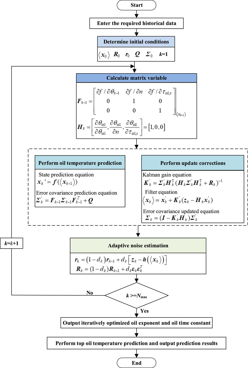
Figure 1. Flow chart of TOT prediction based on the proposed AEKF algorithm.

4 Case analysis

Two main transformers of a provincial substation are taken as the research object. Both are three-phase transformers with oil natural air natural (ONAN) cooling type. Figure 2 shows the field photo of the transformer entity. The rated voltage on the high-voltage side is 110 kV, that on the low-voltage side is 10.5 kV, and the rated capacity is 50 MVA. The transformer key parameters used in the case study are shown in Table 1. These data came from the transformer nameplate and the factory test.

Figure 2

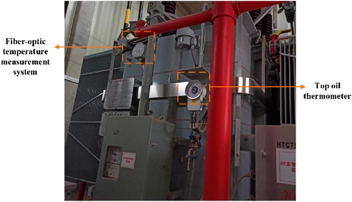
Figure 2. Field photo of the transformer entity.

Table 1

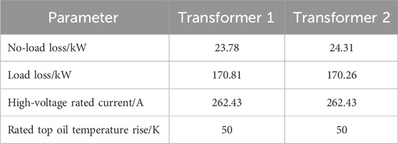
Table 1. Two transformers’ key parameters.

Historical measurements of the TOT are taken from the fiber-optic temperature measurement system installed on the transformers. The fiber optic temperature probe has a temperature range of −80–200°C and a measurement accuracy of ±1°C. The transformer load data is obtained from the Energy Management System (EMS) of the power grid, with a 15-min collection interval. The ambient temperature data is sourced from the National Meteorological Information Center. It provides ambient temperature for every hourly interval, and the temperature at the other moments in between can be achieved by an interpolation method. The algorithm is assessed with δt = 15min, and the initial values of correction parameters are set as n₀ = 0.8, τ_oil,r0 = 360, R₀ = (100)², and diag (Q) = [10⁻³, (0.005/3)², (4/3)²].

4.1 Intraday ultra-short-term prediction results for top oil temperature

The intraday ultra-short-term prediction for the TOT is carried out with the future 15 min as the time scale, which is used for the intraday fault warning and emergency optimization scheduling of the substation.

The proposed method is used to achieve the intraday ultra-short-term prediction of the TOT. Firstly, the updated iterative training on the model is performed according to the historical data set, and the Jacobian matrix is calculated after entering the ambient temperature and the current. Then, the predicted TOT value after 15 min and the measured TOT value is entered into the updated correction model to estimate the state variables (θ_oil, n and τ_oil,r). Next, the observed values and state variables are used to conduct the noise statistical parameter estimation. Subsequently, repeat the above steps to predict the TOT at the next 15-min node, and so on. The optimized values for the state variables of transformer 1 are displayed in Figure 3, where the values of n and τ_oil,r are converged to 1.05 and 540 min, respectively. For transformer 2, the corresponding estimates converge to 1.11 and 570 min, respectively.

Figure 3

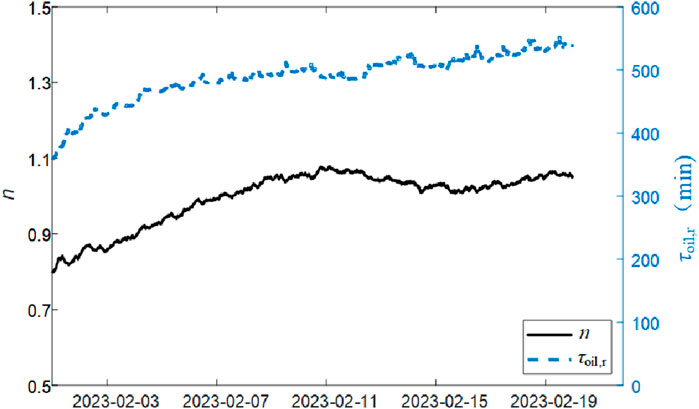
Figure 3. Iterative variation plots of parameters n and τ_oil for transformer 1.

To further reflect the differences between the proposed algorithm and the conventional thermal model, the prediction results using the proposed algorithm and the calculation results using the D. Susa thermal model are compared with the actual TOT values of transformers 1 and 2, as shown in Figure 4. It can be seen that compared with the D. Susa thermal model, the ultra-short-term prediction results by the proposed method are more consistent with the actual values.

Figure 4

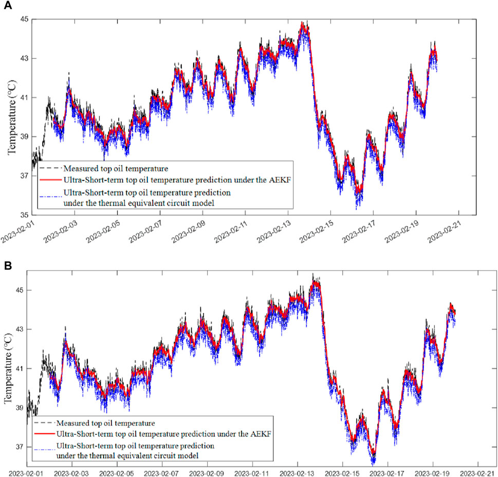
Figure 4. Comparison of intraday ultra-short-term prediction results for TOT by two methods: (A) Intraday ultra-short-term prediction results for TOT of transformer 1; (B) Intraday ultra-short-term prediction results for TOT of transformer 2.

Table 2 shows the root-mean-square errors between the two transformers’ prediction results and actual values under the two methods are calculated according to the statistical data results. It is shown that, regardless of the transformer when the D. susa thermal model is used to predict the TOT, the root-mean-square errors are higher than that of the AEKF algorithm. The main reason is that both oil exponent n and the rated oil time constant τ_oil,r used in the D. Susa thermal model are taken as an empirical value, which are not reliable. For the ONAN transformer, the empirical value of the oil exponent n is 0.25. However, according to the iteration with the AEKF algorithm, the optimized values of n for the two transformers are stable at about 1.05 and 1.11, respectively. For the rated oil time constant τ_oil,r, with the aid of the calculation method in the IEEE standard (IEEE Std C57.91, 2011), the mass and oil volume in different parts of the transformers are substituted to calculate the thermal capacity and then the τ_oil,r can be calculated, which is about 210 min. However, according to the iteration with the AEKF algorithm, the corresponding values of τ_oil,r for the two transformers are stabilized at about 540 min and 570 min, respectively.

Table 2

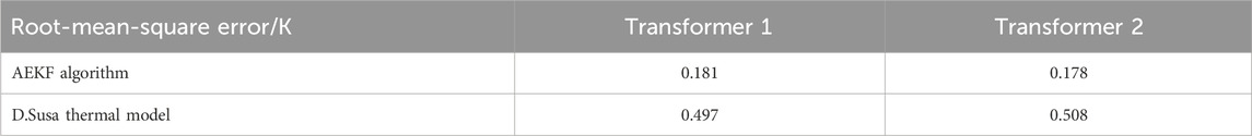
Table 2. Root-mean-square errors of intraday ultra-short-term prediction results for TOT by two methods.

When using the proposed AEKF method, the maximum error is 0.67K, the maximum error percentage is 1.67% and the average error percentage is 0.35% for transformer 1. For transformer 2, the maximum error is 0.63K, the maximum and average error percentages are 1.63% and 0.34%, respectively. The results of the intraday ultra-short-term prediction of the TOT meet the needs of practical engineering calculation.

4.2 Day-ahead short-term prediction results for top oil temperature

The short-term prediction for TOT is carried out with the future 24 h being the time scale. Compared with the intraday ultra-short-term (15 min) prediction, the day-ahead short-time prediction often involves a large error, but it is of vital practical significance for the day-ahead optimization scheduling of the power grid. The TOT short-term prediction can not only provide important data support for the subsequent transformer load state assessment work but also provide the day-ahead temperature data reference when the transformer may appear overloaded so that there will be more response time. The existing machine learning algorithms can only achieve good results in ultra-short-term prediction as they are limited to the time interval of training data and the inevitable impact of the observation noise in the data. By contrast, the method proposed in this paper uses the AEKF algorithm to optimize the model parameter and performs the adaptive estimate on the observation noise. Therefore, it enables a more accurate prediction of the day-ahead TOT.

While the model was constantly iterated and updated according to the continuous observation data, the ambient temperature and current of the next day were entered at 24:00 every day based on the trained model. It can obtain the TOT change curves on the incoming day and record the data, which lasts a total of 19 days. The prediction curves on each of these 19 days are connected to get the full-course TOT observation curve. The short-term prediction results under the proposed algorithm and those obtained using the D. Susa thermal model are compared with the actual values. Figure 5 shows the obtained TOT prediction curves as well as the measurement curves of the two transformers.

Figure 5

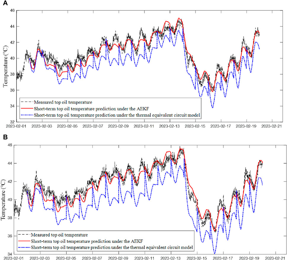
Figure 5. Comparison of day-ahead short-term prediction results for TOT by two methods: (A) Day-ahead short-term prediction results for TOT of transformer 1; (B) Day-ahead short-term prediction results for TOT of transformer 2.

The short-term prediction results are spliced from the prediction results of each day, at the beginning of each day, the TOT prediction value is changed back to the actual value, resulting in a certain fluctuation in the prediction curve, particularly significant in the short-term prediction curve by the D. Susa thermal model. Due to the unreliable thermal parameters and the parameter value being not corrected in real-time in the D. Susa thermal model, the errors gradually increase over time and deviate from the actual values. By contrast, the accuracy of the AEKF algorithm is much higher in the short-term prediction, and the corresponding prediction curve is more coherent. It is seen in Figure 5 that the results from the first several days under the AEKF algorithm are less accurate than those from the several subsequent days. This is because the model is not trained enough during the first several days. It becomes more and more stable over time, so the accuracy of predictions is getting increasingly higher.

To compare the accuracy of the short-term prediction results between the two methods more intuitively, the root-mean-square errors of the two methods are calculated according to the statistical data results, as shown in Table 3. In Table 3, the errors of the short-term prediction under the AEKF algorithm increase to a certain extent relative to the ultra-short-term prediction. For transformer 1, the error increases from 0.181K to 0.541K, with an increase of 0.36K. However, the error of the thermal equivalent circuit model increases from 0.497K in the ultra-short-term prediction to 1.74K in the short-term prediction, with an increase of 1.243K, and the growth rate is about 3.5 times that under the AEKF algorithm. The accuracy in the TOT prediction by the proposed method is superior to that of the D. Susa thermal model at a longer time scale.

Table 3

Table 3. Root-mean-square errors of day-ahead short-term prediction results for TOT by two methods.

When the AEKF method is used for the day-ahead short-term prediction of the TOT, the maximum error is 1.43 K, the maximum error percentage is 3.64%, and the average error percentage is 1.09% for transformer 1. For transformer 2, the maximum error is 1.44 K, the maximum and average error percentages are 3.59% and 1.15%, respectively. It is seen that the calculation results still meet the actual engineering requirements.

4.3 Comparison with the EKF algorithm

Compared with the existing KF algorithm for predicting the TOT, the AEKF algorithm is improved. Specifically, it contains an adaptive estimation of the unknown noise parameters in the recursion process, and then the estimated parameters are used to recurse the solution to the AEKF algorithm. It solves the problem in the original algorithm that the state migration noise and the observation noise as well as their respective covariance matrix are often unknown in the actual application process. Besides, using this method, the noise estimates can be dynamically adjusted over time to ensure the timeliness of the model, thereby further improving the accuracy and practicality of predictions.

In the improved adaptive algorithm, the estimation of the migration noise coordinate matrix Q is removed to ensure the robustness of the algorithm, with only the estimation of the observation noise covariance matrix R_k reserved. Therefore, to better reflect the difference between the AEKF algorithm and the EKF algorithm in the TOT prediction, different initial R_k values, namely, the value of R₀, are taken here to compare the accuracy results of the day-ahead predictions by the two methods. In the case of R₀ = 10², the comparison of short-term prediction results on February 19th by the AEKF algorithm and the EKF algorithm is shown in Figure 6.

Figure 6

Figure 6. Comparison of the day-ahead short-term prediction results of the AEKF and EKF algorithm.

In Figure 6, it is seen intuitively that the short-term prediction results of the AEKF algorithm are superior to those of the EKF algorithm. The root-mean-square error of the prediction curve under the AEKF algorithm is 0.305K, and the maximum error is 0.666K. Under the EKF algorithm, the root-mean-square error is 0.692K, and the maximum error is 1.394K. From these data, it shows that there will be a larger error in the EKF algorithm if the initial value of R_k is incorrectly set. By contrast, the AEKF algorithm can make an adaptive adjustment to R_k, thereby minimizing the deviation caused by the incorrect setting of the initial value. Furthermore, the day-ahead short-term prediction for the TOT is carried out on transformer 1 under the two methods with different R₀ values, the root-mean-square errors between the final results and the real values are displayed in Table 4.

Table 4

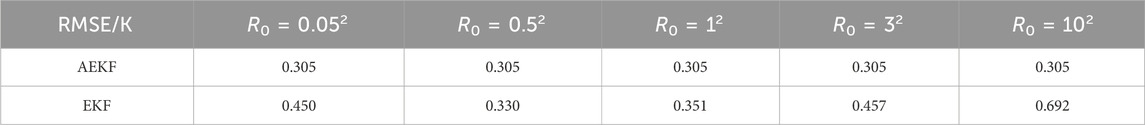
Table 4. Root-mean-square errors of day-ahead short-term prediction of two algorithms with different R₀ values.

With different R₀ values, the AEKF algorithm could always make an adaptive estimation of the noise parameters, and adjust the R_k during each iteration, so that the R_k is closer to the real value, thus ensuring the prediction model has a higher accuracy. While under the EKF algorithm, this could not be realized, the more the R₀ value deviates from the real value, the lower the accuracy of the prediction results would be.

5 Conclusion

Based on the AEKF algorithm, this paper establishes the TOT prediction model at multiple time scales for oil-immersed transformers. The oil exponent, the oil time constant, and the transformer’s TOT are taken as the state variables. The purpose is to simulate the uncertainty in the transformer quality and thermal performance of the material. The corresponding prediction results at different time scales for two transformers are compared with the measured TOT data, proving the effectiveness of the proposed algorithm. The conclusions are as follows:

1) In the intraday ultra-short-term prediction for the TOT, the root-mean-square errors of the TOT prediction curves using the proposed method are 0.181K and 0.178K, respectively, which are less than that obtained by the D. Susa thermal model. It shows that the proposed algorithm has a high accuracy in TOT prediction at a short time scale.

2) In the day-ahead short-term prediction for the TOT, the root-mean-square errors of the TOT prediction curves using the proposed method are 0.541K and 0.561K, which are far less than those obtained by the D. Susa thermal model. It shows that the proposed algorithm still has a high accuracy even in the TOT prediction at a longer time scale.

3) When the proposed AEKF method is used for the prediction of the TOT, the relative error percentage of the intraday ultra-short-term prediction results is less than 2%, and the error percentage of the day-ahead short-term prediction results is less than 4%. The calculation results under both time scales meet the actual engineering calculation requirements.

4) Compared with the EKF algorithm, the adaptive estimation of the noise parameter through the iteration process by the proposed method ensures the accuracy of the prediction model while reducing the requirements on the accuracy of the initial value of the noise parameter. In the day-ahead short-term prediction for the TOT, the accuracy of the EKF algorithm is worse than that obtained by the adaptive optimization algorithm in this paper, no matter how the initial value of the observation noise covariance R₀ of the EKF is specified. The results show that the proposed AEKF method has better robustness and adaptivity.

Data availability statement

The original contributions presented in the study are included in the article/Supplementary Material, further inquiries can be directed to the corresponding author.

Author contributions

YL: Methodology, Writing–original draft. LW: Methodology, Writing–original draft. JJ: Methodology, Writing–original draft. DL: Software, Writing–review and editing. SL: Software, Writing–review and editing. JL: Validation, Writing–review and editing. YL: Validation, Writing–review and editing. WS: Writing–review and editing. MS: Writing–review and editing.

Funding

The author(s) declare that financial support was received for the research, authorship, and/or publication of this article. This research was funded by Science and Technology Project of China Southern Power Grid Company Limited (Research on state recognition technology of power grid equipment based on advanced computing and deep learning), grant number GDKJXM20220318 (036100KK52220031). The funder was not involved in the study design, collection, analysis, interpretation of data, the writing of this article, or the decision to submit it for publication.

Conflict of interest

Authors YL, LW, JJ, SL, and MS were employed by Electric Power Research Institute of Guangdong Power Grid Co., Ltd. Authors DL, JL, and WS were employed by Guangdong Power Grid Co., Ltd. Author YL were employed by China Southern Power Grid Co., Ltd.

Publisher’s note

All claims expressed in this article are solely those of the authors and do not necessarily represent those of their affiliated organizations, or those of the publisher, the editors and the reviewers. Any product that may be evaluated in this article, or claim that may be made by its manufacturer, is not guaranteed or endorsed by the publisher.

References

Alvarez, D. L., Rivera, S. R., and Mombello, E. E. (2019). Transformer thermal capacity estimation and prediction using dynamic rating monitoring. IEEE Trans. Power Deliv. 34, 1695–1705. doi:10.1109/tpwrd.2019.2918243

CrossRef Full Text | Google Scholar

Chen, W., Pan, C., and Yun, Y. (2009). Power transformer top-oil temperature model based on thermal–electric analogy theory. Eur. Trans. Electr. Power 19, 341–354. doi:10.1002/etep.217

CrossRef Full Text | Google Scholar

Chen, W., and Su, X. (2013). Application of Kalman filter to hot-spot temperature monitoring in oil-immersed power transformer. IEEJ Trans. Electr. Electron. Eng. 8, 322–327. doi:10.1002/tee.21862

CrossRef Full Text | Google Scholar

Dong, X., Jing, L., Tian, R., and Dong, X. (2023). Prediction method of transformer top oil temperature based on LSTM model. J. Electr. Power 38, 38–45. ( in Chinese).

Google Scholar

Hartana, P. (2000). Comparison of linearized and extended Kalman filter in GPS aided inertial navigation system. Carleton University.

Google Scholar

He, Q., Si, J., and Tylavsky, D. J. (2000). Prediction of top-oil temperature for transformers using neural networks. IEEE Trans. Power Deliv. 15, 1205–1211. doi:10.1109/61.891504

CrossRef Full Text | Google Scholar

IEC 60076–7 (2017). Power transformers – Part 7: loading guide for mineral-oil-immersed power transformers, 1–89.

Google Scholar

IEEE Std C57.91 (2011). IEEE guide for loading mineral-oil-immersed transformers and step-voltage regulators. IEEE Std C5791-2011 (Revis. IEEE Std C5791-1995), 1–123.

Google Scholar

Lachman, M. F., Griffin, P. J., Walter, W., and Wilson, A. (2003). Real-time dynamic loading and thermal diagnostic of power transformers. IEEE Trans. Power Deliv. 18, 142–148. doi:10.1109/tpwrd.2002.803724

CrossRef Full Text | Google Scholar

Lai, W., Luo, H., Li, W., Cao, Y., Ye, L., and Wang, Y. (2017). “Prediction of top oil temperature for oil-immersed transformer based on Kalman filter algorithm,” in 2017 2nd international conference on power and renewable Energy (ICPRE) (IEEE), 132–136.

CrossRef Full Text | Google Scholar

Li, S., Xue, J., Wu, M., Xie, R., Jin, B., Wang, K., et al. (2021). “Prediction of transformer top oil temperature based on improved weighted support vector regression based on particle swarm optimization,” in 2021 international Conference on advanced electrical Equipment and reliable operation (AEERO) (IEEE), 1–5.

Google Scholar

Liu, Y., Li, X., Li, H., Yin, J., Wang, J., and Fan, X. (2022). Spatially continuous transformer online temperature monitoring based on distributed optical fibre sensing technology. High. Volt. 7, 336–345. doi:10.1049/hve2.12031

CrossRef Full Text | Google Scholar

Sage, A. P., and Husa, G. W. (1969). Adaptive filtering with unknown prior statistics. Jt. Autom. Control Conf. (7), 760–769.

Google Scholar

Shiravand, V., Faiz, J., Samimi, M. H., and Mehrabi-Kermani, M. (2021). Prediction of transformer fault in cooling system using combining advanced thermal model and thermography. IET Generation, Transm. Distribution 15, 1972–1983. doi:10.1049/gtd2.12149

CrossRef Full Text | Google Scholar

Sönmez, O., and Komurgoz, G. (2018). “Determination of hot-spot temperature for ONAN distribution transformers with dynamic thermal modelling,” in 2018 condition monitoring and diagnosis (CMD) (IEEE), 1–9.

Google Scholar

Susa, D., Lehtonen, M., and Nordman, H. (2005a). Dynamic thermal modelling of power transformers. IEEE Trans. Power Deliv. 20, 197–204. doi:10.1109/tpwrd.2004.835255

CrossRef Full Text | Google Scholar

Susa, D., Lehtonen, M., and Nordman, H. (2005b). Dynamic thermal modeling of distribution transformers. IEEE Trans. Power Deliv. 20, 1919–1929. doi:10.1109/tpwrd.2005.848675

CrossRef Full Text | Google Scholar

Tan, F., Zhu, C., Xu, G., Chen, H., and He, J. (2022). Method of UHV transformer top oil temperature forecasting based on decoupling analysis and Euclidean distance. High. Volt. Eng. 48, 298–306. (in Chinese).

Google Scholar

Wang, K., Zhang, H., Wang, X., and Li, Q. (2020a). “Prediction method of transformer top oil temperature based on VMD and GRU neural network,” in 2020 IEEE international conference on high voltage engineering and application (ICHVE) (IEEE), 1–4.

CrossRef Full Text | Google Scholar

Wang, L., Zhang, X., Villarroel, R., Liu, Q., Wang, Z., and Zhou, L. (2020b). Top-oil temperature modelling by calibrating oil time constant for an oil natural air natural distribution transformer. IET Generation, Transm. Distribution 14, 4452–4458. doi:10.1049/iet-gtd.2020.0155

CrossRef Full Text | Google Scholar

Wang, L., Zhou, L., Yuan, S., Wang, J., Tang, H., Wang, D., et al. (2019). Improved dynamic thermal model with pre-physical modeling for transformers in ONAN cooling mode. IEEE Trans. Power Deliv. 34, 1442–1450. doi:10.1109/tpwrd.2019.2903939

CrossRef Full Text | Google Scholar

Wu, J., Zhou, Z., Fourati, H., Li, R., and Liu, M. (2019). Generalized linear quaternion complementary filter for attitude estimation from multisensor observations: an optimization approach. IEEE Trans. Automation Sci. Eng. 16, 1330–1343. doi:10.1109/tase.2018.2888908

CrossRef Full Text | Google Scholar

Zhang, L., Luo, Y., Sheng, G., Ni, Z., and Jiang, X. (2024). Improving IEC thermal model for oil natural air natural transformers using optimised parameters based on dynamic simulation. High. Volt. 9, 217–229. doi:10.1049/hve2.12374

CrossRef Full Text | Google Scholar