Modeling the hydrodynamic wake of an offshore solar array in OpenFOAM

Offshore solar is seen as a promising technology for renewable energy generation. It can be particularly valuable when co-located within offshore wind farms, as these forms of energy generation are complementary. However, the environmental impact of offshore solar is not fully understood yet, and obtaining a better understanding of the possible impact is essential before this technology is applied at a large scale. An important aspect which is still unclear is how offshore solar affects the local hydrodynamics in the marine environment. This article describes the hydrodynamic wake generated by an offshore solar array, arising from the interaction between the array and a tidal current. A computational fluid dynamic (CFD) modeling approach was used, which applies numerical large eddy simulations (LES) in OpenFOAM. The simulations are verified using the numerical model TUDFLOW3D. The study quantifies the wake dimensions and puts them in perspective with the array size, orientation, and tidal current magnitude. The investigation reveals that wake width depends on array size and array orientation. When the array is aligned with the current, wake width is relatively confined and does not depend on the array size. When the array is rotated, the wake width experiences exponential growth, becoming approximately 30% wider than the array width. Wake length is influenced by factors such as horizontal array dimensions and current magnitude. The gaps in between the floaters decrease this dependency. Similarly, the wake depth showed similar dependencies, except for the current magnitude, and only affected the upper meters of the water column. Beneath the array, flow shedding effects occur, affecting a larger part of the water column than the wake. Flow shedding depends on floater size, gaps, and orientation.

1 Introduction

The development and utilization of concepts for energy production from renewable, clean, and sustainable sources are essential to decrease our dependency on fossil fuels (Renewables Now, 2018). Simultaneously, the easily accessible natural reserves of fossil fuels are reaching its end. As a result, substantial developments have taken place in the past years to harvest energy from solar and wind sources. Utilizing them remains a challenge, as space on land is limited and is often in conflict with other uses (Oliveira-Pinto and Stokkermans, 2020; Song et al., 2022). This all leads to a shift toward offshore energy generation, where oceans and shelf seas are perceived as an excellent opportunity to harvest untapped energy (Kumar et al., 2015).

One of these renewable energy concepts is offshore floating photovoltaics, which will be referred to as offshore solar. Offshore solar has significant potential to address the energy demand by supplying clean energy (Group and Esmap. 2019). The smaller spatial footprint of solar energy compared to offshore wind, attributed to its relatively high yield (Kumar et al., 2015), makes it suitable for co-location within offshore farms. These sources of energy are complementary (Golroodbari et al., 2021), leading to less volatile offshore energy production (Nassar et al., 2020; Zheng et al., 2020; Koundouri et al., 2021; Ruzzo et al., 2021). Hence, the potential of offshore solar is evident.

Before deploying offshore solar on a large scale, its effect on the marine ecosystem must be carefully considered (Karpouzoglou et al., 2020; Hooper et al., 2021; Mavraki et al., 2023; Vlaswinkel et al., 2023; Benjamins et al., 2024). Assessing the ecosystem impacts of offshore solar is a complex process, as it has both direct and indirect effects, which are often related. These effects may be oppositely directed (Vlaswinkel et al., 2023).

This study focuses on an offshore solar array consisting of thin rectangular floaters floating on the water surface (illustrated in Figure 1). They represent the design of offshore solar developer Oceans of Energy, which has deployed such a pilot array in the southern North Sea. A previous study on the impact of large-scale floating solar (Karpouzoglou et al., 2020) found that the hydrodynamics beneath the farm can change significantly due to wind shielding and platform friction. The foreseen effect is the generation of a hydrodynamic wake and goes along with various flow phenomena such as boundary layer development and flow shedding. These phenomena affect the shape of the hydrodynamic wake. Within the wake, flow velocity changes and affects the turbulent mixing. The interaction may disrupt the natural stratification, i.e., the vertical layering of the water column, due to density differences. The exact effect of large-scale floating solar arrays on stratification patterns is still uncertain and requires more field and modelling research studies (Karpouzoglou et al., 2020). As stratification controls the vertical distribution of algae, nutrients, and oxygen, it is one of the key abiotic factors controlling marine ecosystem functioning (Daewel et al. (2022)).

Figure 1

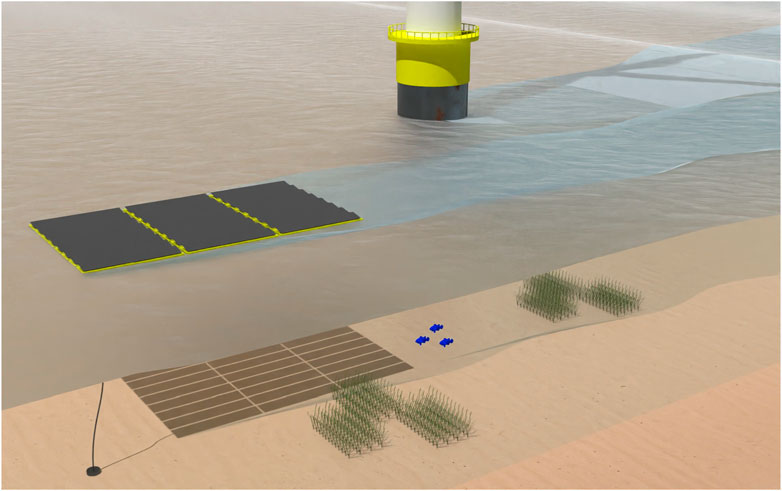
Figure 1. Hydrodynamic wake of a cluster of floaters in the current interacting with the environment: e.g., seagrasses, fish, and monopile and its wake. The hydrodynamic wake is highlighted. This article focuses on this configuration.

Despite the abundance of literature focusing on turbulent wakes produced by cylindrical objects applicable to offshore technology (Karniadakis and Triantafyllou (1992); Miles et al. (2017); Chen and Christensen (2018)), research on hydrodynamic wakes generated by thin floaters remains relatively sparse, with a primary emphasis on boundary layer theory (Schlichting and Gersten, 2016) and experimental investigations (Knisely, 1990; Hemmati et al., 2017; D’ıaz-Ojeda et al., 2019; Rostami et al., 2019). The authors are not aware of studies that consider the hydrodynamic wake of thin floaters with a relatively high size–thickness ratio and their individual rotation effects compared to the current direction.

This article aims to quantify the dimensions of a hydrodynamic wake generated by an offshore solar array and provides initial insights into the hydrodynamic wake and unsteady flow characteristics around the array, as illustrated in Figure 1. The study examines the effect of array orientation and current magnitude on the hydrodynamic wake, offering valuable insights into how these affect the wake size. These findings can be utilized for contrasting various foreseen impacts of (large-scale) offshore solar on marine ecosystems in combination with the (hydrodynamic) effects of offshore wind turbines. The outcomes can be used to address a part of the mentioned knowledge gap regarding the effect of a large-scale offshore solar array on stratification.

2 Methodology

2.1 Numerical model

The flow around the offshore solar array is modeled by using the open-source computational fluid dynamic (CFD) software package OpenFOAM (OpenCFD, 2004) version 8. Earlier work showed that this model can simulate adequately turbulent flow over a thin plate (Kim et al., 2019; Sanjay et al., 2019).

A one-phase solution is chosen for simulating the impact of the solar array on local and surrounding hydrodynamics. The fluid solver (pimpleFOAM) solves the incompressible Navier–Stokes equations for each grid cell using the finite volume discretization method. The variables pressure and velocity have a collocated arrangement. The PIMPLE algorithm is used to solve the system of equations. A forward Euler time discretization scheme is used, and in space, a second-order upwind scheme is applied. A Courant–Friedrichs–Lewy (CFL) number equal to 1.0 is chosen based on a pre-assessment to ensure numerical stability and is low enough to capture frequency-related shedding effects.

Large-scale turbulence is modeled using large eddy simulation (LES), while the smaller isotropic turbulent scales, which are smaller than the grid cell size, are modeled with the subgrid model dynamic k-equation (Kim and Menon, 1995) along with the Van Driest damping function close to the array. The LES simulations are initialized using the flow field from a precursor simulation. For this precursor simulation, a Reynolds-averaged Navier–Stokes (RANS) approach is applied. The RANS approach does not provide an as accurate turbulence representation as LES but is less computationally demanding. The RANS simulations are initialized with a turbulence intensity of 3% and are stopped until the solution reaches a steady state. The kω-SST model is used to model the turbulence for all scales, which is suitable for determining the boundary layer development on a thin plate (Sanjay et al., 2019).

The validation of the numerical results is currently not possible due to the lack of field data. An alternative numerical approach is used for comparison to allow for reflection on the obtained results. The OpenFOAM simulations are verified by comparing them with additional CFD simulations using the TUDFLOW3D model (De Wit et al., 2015; 2023), which also uses LES. Although the OpenFOAM simulations focus more on the local flow details around the array, LES with TUDFLOW3D is applied with a finer resolution in the far field. The advantage of this denser grid in the wake is an accurate estimation of the energy decay of the turbulence to smaller eddy scales. A second-order Adams–Bashforth time stepping scheme and the AV6 advection scheme for the convective term are used (de Wit and van Rhee, 2014). The one-step projection method is applied with a CFL number of 0.5. The turbulence subgrid model used is the WALE model (Nicoud and Ducros, 1999). The array is represented using an immersed boundary method.

The applied numerical software packages OpenFOAM and TUDFLOW3D have been validated for flow benchmarks where experimental data were available (De Wit, 2015).

2.2 Schematization of offshore solar arrays and boundary conditions

The offshore solar array is schematized into a series of floaters in an 8 by 3 configuration, with gaps between the individual floaters (Figure 1). The array dimensions are indicated with L, W, and d for length, width, and submerged depth, respectively. The floater length is almost 0.33 L, with the gap size 2.67% in the floater length. The array is assumed to be fixed in place. The effect of waves is not part of this study in order to reduce computational costs.

The sides and bottom of the numerical domain are confined by a smooth wall with a free-slip condition. The top consists of a rigid-lid boundary. A velocity U is uniformly imposed at the inlet, while at the outlet, a normal pressure gradient equal to 0 is imposed to reduce backward forcing in case the wake is not fully developed. No-slip conditions are applied for the array surfaces. A low-Reynolds boundary approach has been applied at the array surfaces in combination with a small grid spacing. For water, a kinematic viscosity (ν) of 1e-6 m²s⁻¹ is applied. The duration of the simulations is chosen such that the flow passes the total domain two times.

2.3 Numerical domains

Two numerical domains are used in this study, which will be further referred to as the “wide 3D” and “narrow 3D” domains. The wide 3D domain illustrated in Figure 2A is used to investigate the wake width and three-dimensional flow phenomena around the array. The narrow 3D domain in Figure 2B is used to investigate the wake length and depth and is extended in length compared to the wide 3D domain. The narrow 3D grid is the same as the cross-section of the wide 3D domain.

Figure 2

Figure 2. (A) 3D grid view: wide 3D domain. (B) Side grid view: narrow 3D domain. Domain with dimensions showing close-ups of grid resolution.

A quadrilateral grid is used as the basis to achieve an aspect ratio of 1 for each grid cell in the domain, which is preferable for LES simulations. The base grid of the wide 3D domain, which is the coarsest region, has a length of approximately 0.04 L per cell in each direction. Every refinement region is created with a factor of 2, resulting in five regions in total and a grid cell length of below 0.0015 L near the array. Similarly, the narrow 3D grid has four regions and a base cell length of 0.02 L. The third dimension has a width of 0.24 L. To solve the boundary layer with both domains, 10 prism layers with a thickness ratio of 1.3 are added, resulting in a first cell height of 2.2e-5L at the floaters. This results in a grid of 7.2 million cells for the wide 3D domain and 2.5 million cells for the narrow 3D domain.

The 3D LES simulations with TUDFLOW3D use a uniform grid with a constant spacing of 0.002 L in the horizontal direction and 0.001 L in the vertical direction. This results in a grid of 18 million cells. Numerical details on TUDFLOW3D can be found in De Wit (2015). At the array, the grid is less refined than in the model used for OpenFOAM.

2.4 Parametrization and quality assessment

In numerical modeling, ensuring independence of results from spatial and temporal discretization is crucial. Turbulent feature resolution with LES simulations is particularly sensitive to discretization. For this study, sensitivity analyses on spatial and temporal discretization have been conducted to ensure accurate results. For investigating the influence of overall spatial discretization on results, different grid resolutions are tested via time-averaging in the narrow 3D domain. A concise overview of the sensitivity and convergence study is provided in the Supplementary Material.

The grid refinement around floaters was analyzed separately to accurately capture boundary layer development and flow detachment. Grid resolution was optimized to keep the dimensionless wall distance (y⁺) below 5. Lower values for y⁺ are not needed if low-Reynolds wall functions are utilized on the floater surface. This is done to maintain resolution without inflating computational costs, even though a wall function relies on assumptions. Refinement into the semi-viscous logarithmic part of the boundary layer was necessary and has been shown to capture flow characteristics consistently. The chosen wall function takes the velocity distribution near the surface based on hydraulic rough flow into account (Dey, 2014). The roughness is within the order of the nearest grid cell size. The sensitivity of applying different wall functions, including increase in roughness, is discussed in the Supplementary Material.

As shown in Figure 2A, the gaps in between the rectangular floaters of the array are significantly smaller in comparison to the overall extent of the floaters. The effect of the gaps has been investigated to explore the necessity of detailed modeling. The LES simulations show an influence on the local velocity profile near the gap due to the smaller boundary layer thickness. The development of time-dependent turbulent features in the form of vortex shedding was affected. Consequently, the gaps have been included into further investigation.

2.5 Simulation overview

A total of 10 simulations are conducted with the LES approach, as illustrated in Table 1. The rotation of the array (α), current magnitude (U), and array length (L) for the two different numerical grids are varied among these simulations. The variation in the velocity is expressed with the dimensionless Reynolds number (Re_L = UL/ν). The verification using TUDFLOW3D has been performed for the narrow 3D cases. The submerged depth (d) of the floaters has not been varied, as the influence is expected to be small on the development of the wake in comparison to the array position and dimensions.

Table 1

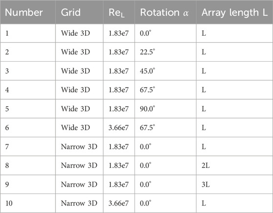
Table 1. List of simulations performed. TUDFLOW3D is performed for the narrow 3D cases.

The results of the simulations in this study are presented in contour plots based on the data averaged over 100 time frames with a frequency of 1 Hz. Therefore, the data in horizontal planes are analyzed at three different water depths, $1\frac{1}{3}$d, $2\frac{2}{3}$d, and 4 d below the water surface and plotted as contours. A vertical plane aligned with the current direction is analyzed as well.

For the wide 3D domain, the velocity is sampled along a vertical line beneath the array until a depth of $16\frac{2}{3}$d. The distribution of the probing points is arranged logarithmically. Velocity information is obtained over a total of 1,000 time frames with a frequency of 10 Hz, which is sufficient to capture time-dependent flow separation. The probe positions in the horizontal space are indicated by the green crosses in Figure 2A.

3 Results

3.1 Analytical definition of the hydrodynamic disturbed flow region and wake

In this study, the extent of the disturbed flow is defined by making use of a so-called length-averaged velocity difference U_diff. Thereby, U_diff represents the averaged velocity difference between the local velocity u and the ambient current U over the length h. These flow parameters are related by Equations 1, 2 (Garcia and Parker, 1993):

$U_{diff}h={\int }_0^{x_{\infty }}\left(U-u\right)\mathit{\text{dx}},(1)$

$U_{diff}^{2}h={\int }_0^{x_{\infty }}{\left(U-u\right)}^2\mathit{\text{dx}},(2)$

The following two regions are analyzed: the disturbed flow region beneath the array and the disturbed flow region behind the array. The latter one is defined as the hydrodynamic wake.

For the disturbed region beneath the array, the length h is representative for the determination of the depth that is disturbed beneath the array (h = d_local).

For the hydrodynamic wake, the length h is representative for the determination of the wake depth (h = d_wake) or the horizontal dimensions of the wake width (h = W_wake). The wake length L_wake is determined by following the development of U_diff for the wake depth in the positive x direction. The coordinate at which U_diff is approaching 0 defines this wake length.

Figure 3 presents the flow amplification at and around the solar array in the form of a contour plot for the depth of $1\frac{1}{3}$d below the floater’s bottom. Two figures are presented where one is the averaged field over time while the latter one indicates the vortex shedding effects at one time instance. The contour marks the velocity contour for a 5% decrease in velocity in comparison to the ambient current (U). The red markers indicate the resulting data points marking the wake width (W_wake), which are obtained after the integration described in Equations 1, 2.

Figure 3

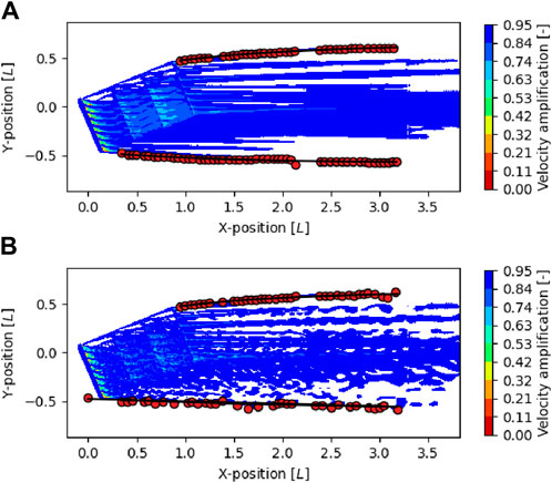
Figure 3. (A) Averaged flow amplification, averaging the shedding effect over time. (B) Instantaneous flow amplification illustrating the vortex shedding on one time instance. Contours of the velocity amplification at $1\frac{1}{3}$d below the free surface for a 22.5° orientation and Re_L = 1.83e7. The data points for the characteristic length W_wake ( ) found after the integration are included.

3.2 Disturbed flow region beneath the array

Figure 4 presents the flow field around the upstream floater of the array. The immersion of the floater results in a small area of decreased velocity upstream of the floater front and leads to flow separation and vortex shedding due to the sharp corner of the floater. After the flow is reattached, a boundary layer flow development becomes apparent. Thus, the local depth d_local of the disturbed flow beneath the solar array is affected by 1) boundary layer development and 2) turbulent features due to flow shedding.

Figure 4

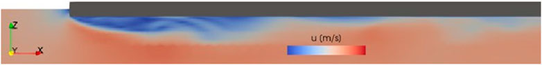
Figure 4. Flow field represented by the flow velocity magnitude u at the first floater of the solar array for an orientation of 0°.

3.2.1 Boundary layer development

The vertical velocity profiles of the flow field beneath the array are analyzed for the development of the boundary layer. These profiles are obtained at the locations defined in Figure 2A. Figure 5 presents the time-averaged flow profiles at five locations along the x-direction for the solar array with an orientation of 0°. Thereby, the flow profiles of the OpenFOAM simulations with the RANS and LES as well as the TUDFLOW3D simulations with LES are shown.

Figure 5

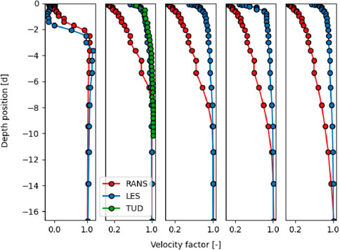
Figure 5. Velocity profile over the depth with α equal to 0° and averaged over 100 time frames. A comparison made with the TUDFLOW3D results. Five locations in the x-direction are provided starting at the front of the array: 0.03, 0.3, 0.5, 0.7, and 0.97 L.

At the first output location, all velocity profiles indicate flow separation due to the adverse velocity. With increasing distance in the x-direction, the flow reattaches, and boundary layer thickness becomes apparent. The velocity profiles obtained from the RANS and time-averaged LES simulations are significantly different where the profiles for the RANS simulation have a smaller velocity gradient in the vicinity of the floaters. Even though the chosen RANS turbulence model k-omega-SST gives accurate results for backward-facing step flow cases and boundary layer development (Sanjay et al., 2019), the total thickness of the boundary layer is significantly larger for the RANS simulations than for the LES simulations. Although the RANS velocity profile shows a boundary layer thickness of up to 16 d at the downstream end of the array, the boundary layer thickness (d_local) for the LES simulations seems to be in the order of 3 d.

The turbulence models used in RANS simulations are linear eddy viscosity models, which can sometimes overestimate boundary layer thickness due to their reliance on simplifying assumptions. When the actual conditions are more complex than these assumptions account for, the result can be significant overestimation. RANS models struggle with the anisotropy of Reynolds stresses caused by larger eddies, such as those originating from flow separation at the front of the array. Consequently, the flow predicted by the RANS model appears unaffected by the gaps between the floaters due to the increased boundary layer thickness. In contrast, the boundary layer thickness predicted by LES is comparable to the gap distance between the floaters. The TUDFLOW3D model, using a relatively coarse grid for the array, produced results similar to those obtained with LES in OpenFOAM, as shown in the second velocity profile of Figure 5.

The exact value of the depth of the disturbed flow beneath the array (h = d_local) is determined by the integration of Equations 1, 2. Beneath the array, a characteristic thickness d_local of $3\frac{1}{3}$d across all array lengths is found, as depicted in Figure 6. This aligns with turbulent boundary layer theory, which predicts a thickness of 5 d for a plate with the length L without gaps (Schlichting and Gersten, 2016). The lower value than the theoretical prediction can be caused by the presence of the gaps. The jump in U_diff at the location of the gaps indicates local flow separation. The depth after each gap decreases before building up again. Notably, the local wake depth remains relatively constant with changes in array length using OpenFOAM.

Figure 6

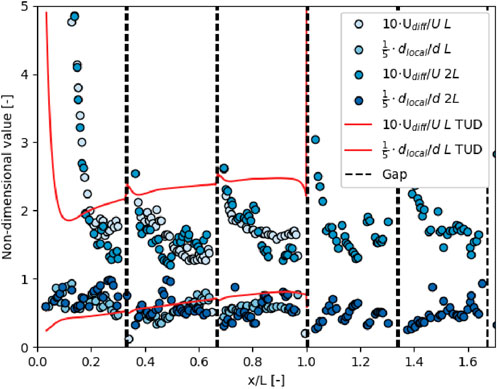
Figure 6. A Disturbed flow region beneath the array averaged for a Re_L equal to 1.83e7.

The results of TUDFLOW3D for U_diff behave more linearly as if the array is a continuous floater without gaps. Each gap in TUDFLOW3D is just four cells in length and three cells in height, which does not allow for much turbulent shedding, which is simulated on the finer OpenFOAM grid. The same is visible for the wake depth d_local and can be explained by the lower grid resolution near the array.

3.2.2 Turbulent features

Flow separation is observed at the sides of the floaters and is affected by the array orientation with respect to the flow direction. It is observed that when the array is positioned in a 0° or 90° orientation with respect to the incoming flow direction, the flow separation also develops symmetrically in the horizontal plane. In the case of an array orientation, which results in a non-symmetric position to the flow direction (22.5°, 45°, and 67.5°), the flow separation is no longer symmetrical but is affected by the alignment of the solar array sides to the flow.

Figure 7 presents the contours of the depth of the disturbed flow field beneath the array and in its wake for the instantaneous flow field. The contours are obtained for a 1% velocity difference with the ambient current U, depicted for two rotations: 22.5° and 67.5°, and illustrate the effect of the rotation on the vortex shedding.

Figure 7

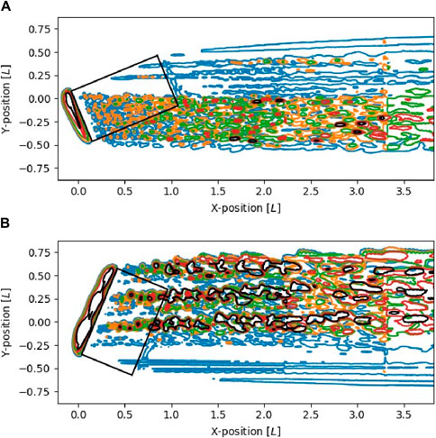
Figure 7. (A) Rotation of 22.5°. (B) Rotation of 67.5°. A disturbed flow region of one time frame and with minimal 1% velocity difference with the ambient current of the array. This is either the length L for one side or the width W for the opposed side. Thus, the wake ambient current is provided for five different water depths: ( ) $5\frac{1}{3}d$, ( ) 10 d, ( ) $13\frac{1}{3}d$, ( ) $16\frac{2}{3}d$, and ( ) 20 d. These figures do illustrate the vortex shedding at one time instance.

The contour plots show that the flow field is significantly affected, particularly at the front edge of the array. In this area, the array blocks the flow upstream, resulting in flow separation, where d_local reaches greater depths for the orientation with 67.5° than for 22.5°. Thereby, the contours indicate that the highest depth is always located at the most upstream corner of the array, while the depth decreases along the leading edge with in flow direction.

In addition, for beneath the array, the orientation with 67.5° results in the deepest disturbed flow patterns larger than 20 d. Downstream of the blockage of the floater, initially small eddies are generated beneath the array. The vortex stretching leads to an increased length of the visible turbulent eddies and a greater depth of the disturbed flow. The variation in the array orientation reveals that the depth of the disturbed flow field not only depends on the array dimensions but also on the angle of attack AoA. The angle of attack is the angle between the edge of the array and the flow direction. The governing dimension seems to be the so-called corner length (L_c), which is the distance from the front of the array to the nearest sideway corner. This could be formulated as follows: d_local = f (AoA, L_c,floater). Since this study used orientation bins of 22.5°, it is unclear if intermediate orientations would result in even greater vertical wake extents.

The depth contours beneath the array further indicate the impact of the gaps between individual floaters. Figure 7B strongly demonstrates the effect of the gaps. The positions of the gaps orthogonal to the flow direction are simultaneously the trajectories of turbulent flow feature transport and co-align with the tracks of the deepest flow disturbance in the disturbed flow region. As displayed in Figure 7A, this effect is less pronounced if the gaps are located closer to each other. In addition, here, the angle of attack and the corner length have an influence on the patterns of turbulent features.

The vortex shedding within the disturbed flow region can be described by the Strouhal number (St), which can be determined from the vortex shedding frequency f. For partially submerged thin plates, the Strouhal number is defined as St = $2\frac{\mathit{fd}}{U}$, where d is the submerged depth and U is the ambient current. The vortex shedding frequency is obtained through a Fourier analysis after removing the mean velocity signal of the velocity probes beneath the array given in Figure 2A.

Figure 8 shows the frequency of vortex shedding for Re_L = 1.83e7 from the narrow 3D domain for different locations in the x-direction.

Figure 8

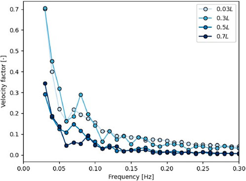
Figure 8. Fourier analysis for Re_L = 1.83e7 for different positions in the x-direction.

For all locations over the array length shown in Figure 8, the results of the Fourier analysis show two peaks. Here, the first peak is related to the mean, and the second peak corresponds to one of the shedding frequencies and in the Fourier frequency domain corresponds to approximately 0.08 Hz (between 0.07 and 0.09 Hz). This is mostly apparent at the x-location of 0.3 L. In the case of a current velocity that corresponds to Re_L = 3.66e7, the second peak emerges at frequency values of 0.08 and 0.17 Hz. The first peak corresponds with a Strouhal number of 0.06. A number in this order aligns with findings in the literature on fully submerged plates, indicating that the Strouhal number can be below 0.1 (Knisely, 1990; Rostami et al., 2019).

3.3 Wake development behind the array

3.3.1 Wake depth and length

Behind the array, the flow detaches, but the flow remains disturbed over a certain distance, as described by the wake behind the array. The vertical extent of the wake behind the array is described by the wake depth (d_wake). This should not be confused with the depth of the disturbed flow beneath the array (d_local).

The results of the wide 3D domain in Figure 7 showed that the wake depth behind the array for x/L > could extend more than 20 d due to the flow-shedding effects near the gaps and vortex stretching. The wake depth for an instantaneous flow field due to the turbulent features generated by the presence of the gaps has similar dependencies as the local depth, being dependent on the corner length and the angle of attack. As shown in Figure 7, the eddies start to dissipate within a couple of lengths L in the wake because the black-colored eddies become less pronounced.

The wide 3D domain is limited in size. To further investigate the development of the wake depth in the x-direction, the time-averaged narrow 3D domain results are used. This is done by looking at both U_diff and d_wake found by Equations 1, 2. The results of these variables are plotted in the x-direction, as shown in Figure 9, where x = 0 is the aft of the array with an orientation of 0°. The trend of U_diff behaves asymptotically, approaching 0. When it approaches 0, it means that the flow is not disturbed anymore. The d_wake seems to converge to a maximum penetration depth.

Figure 9

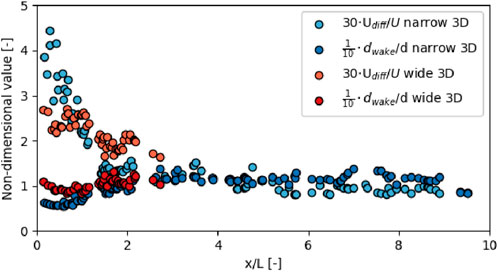
Figure 9. Vertical wake for L and an Re_L equal to 1.83e7, where x starts from the aft of the array. The wide 3D results are compared with the narrow 3D results.

The wide 3D domain, like in Figure 7, and narrow 3D domain are both plotted in Figure 9 for an orientation of 0°. The comparison is made to show that the wide 3D domain cannot provide the trend of U_diff and d_wake while the narrow 3D domain can. The magnitude of the wake depth of approximately 12 d between the two domains matches, arguing that the narrow 3D domain is representative of the wake development. As the wake is still present even at the end of the longer narrow 3D domain, fitting is used for the analysis of the wake.

A subsequent step is to consider the effect of the variations that are discussed in Table 1 on the wake development. The results for U_diff and d_wake are discussed separately. This is to make the distinction that U_diff is used to determine the L_wake when the fit approaches 0, rather than defining d_wake.

First, the effect of increasing the array length on the vertical wake size is analyzed. The results for U_diff and d_wake together with an asymptotic fit in the form of b/x^a are provided, as illustrated in Figure 10A. The legend provides information on the variation, starting with the dimensionless number on the y-axis and ending with the length of the array. In addition to the OpenFOAM LES results, the TUDFLOW3D results are shown by green lines for the verification of the grid resolution in the wake. No distinction is made between the green lines for the sake of clarity.

Figure 10

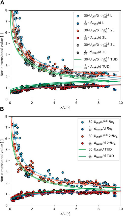
Figure 10. (A) Fit for lengthening the array. (B) Fit for the increase in the ambient current. All fits for the vertical wake for the defined variations. The legend provides information of the variation, starting with the dimensionless number on the y-axis and ending with the length of the array or the current magnitude.

The wake depth d_wake found from the OpenFOAM results is similar for the three different array lengths. In contrast to OpenFOAM, the wake depth results for TUDFLOW3D do show a slight dependency on the array length, whereas TUDFLOW3D in general resulted in a thicker wake d_wake than OpenFOAM of approximately 16 d for x/L > 10, and an increase in array length results for TUDFLOW3D in a variation of the wake depth of approximately 2 d as well. This difference in wake depth between TUDFLOW3D and OpenFOAM originates mostly from x/L = 0, which is relatable to the dependency found in the results for the local wake depth (d_local) in Figure 6. The difference in the inflow generated beneath the array and the grid resolution explains this difference in dependency for OpenFOAM and TUDFLOW3D.

The wake length L_wake is based on U_diff. The U_diff is normalized by n_fac, which represents the factor of increase in length, being 3, 2, or 1 for 3 L, 2 L, and L, respectively. The wake length does dependent on the array length: the 2 L and 3 L array lengths result in a 23% and 39% longer wake length for OpenFOAM, respectively. The U_diff plots and wake length derived from U_diff from OpenFOAM and TUDFLOW3D are close to each other, showing a similar trend for the U_diff decay behind the array. The remaining differences follow from the different start of the wake directly behind the array and the difference in the resolved presence of the gaps in the array. The differences in the dependency of n_fac for OpenFOAM and TUDFLOW3D can be explained for similar reasons.

Furthermore, the effect of increasing the ambient current U from Re_L = 1.83e7 to Re_L = 3.66e7 on the vertical wake development is analyzed. Again, the results for U_diff and d_wake together with an asymptotic fit in the form of b/x^a are provided, as illustrated in Figure 10B. The legend is built up in a similar way as for the array lengthening.

The wake depth d_wake behind the array does not depend on the ambient current. This is the case for both TUDFLOW3D and OpenFOAM results.

The depth-averaged difference velocity U_diff is comparable between OpenFOAM and TUDFLOW3D. Looking at the trend of the fits, TUDFLOW3D shows a slightly larger decay over position. This is likely caused by the denser grid resolution in the wake, which improves the estimation of vortex stretching. As a consequence, the U_diff fit found with the OpenFOAM results will last longer before it reaches near 0 and will lead to a larger estimated L_wake. The results for U_diff do show a dependency on the ambient current U. Therefore, the results for U_diff are normalized by U, where TUDFLOW3D seems to scale with U, OpenFOAM is less dependent, and U^0.8 is assumed. Again, the difference in approach and the less resolved boundary layer beneath the array by TUDFLOW3D, especially at the gaps, can result in a lower turbulent intensity and can explain the initial difference.

After understanding the scaling of U_diff and d_wake for the different variations in the setup discussed, all normalized data are combined, and a final fit to describe the vertical wake development is provided. The fits are illustrated in Figure 11.

Figure 11

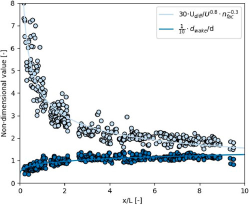
Figure 11. Final fit of all normalized data points using OpenFOAM.

Equation 3 for d_wake is the mean of the OpenFOAM fits:

${\mathit{\text{d}}}_{\mathit{\text{wake}}}=0.67x^{0.17},(3)$

where x in m and with a maximum standard deviation of the coefficients within 2%. The d_wake is continuously growing over the considered domain. In reality we do think the function will change outside the domain and is therefore not suitable for the determination of L_wake. For U_diff , the following fit is found:

$U_{\text{diff}}=0.197x^{-0.406}{U}^{0.8}{L}^{0.3},(4)$

where U and L are in m/s and m, respectively, with a maximum standard deviation of the coefficient within 2%. The fit is asymptotic, but in reality, it is expected that for a sufficiently small U_diff, the wake cuts off and is not present anymore. Verification with a longer numerical domain is required to verify this hypothesis. For the remainder, we assume that this is approximately a 5% difference in U and u.

The wake length L_wake when the velocity u reaches 95% of U is within 10 L for OpenFOAM for Re_L = 1.83e7 and length L. For TUDFLOW, for 95%, L_wake is within 7.2 L. It is worthwhile to mention that the RANS simulations resulted in a wake length being a factor of 2 smaller.

3.3.2 Horizontal wake width

The horizontal wake extent behind the array is quantified by the wake width (W_wake). The wake width W_wake is defined as the additional distance compared to the projected frontal width (W_y) of the array under different orientations, as illustrated in Figure 2A. The total wake width can be calculated by summing Wy with W_wake.

For the determination of the wake width, the time-averaged velocity fields within three horizontal planes at a regular distance in depth ($1\frac{1}{3}$d, $2\frac{2}{3}$d, and 4 d) are analyzed. The wake width is calculated using Equations 1, 2 per x-location for h = W_wake. The red dots in Figure 3A showed exemplarily a resulting time-averaged velocity contour for the plane at a depth of $1\frac{1}{3}$d for the orientation 22.5°.

Figure 12 presents the resulting data points of W_wake over the x-direction for the three water depths and an array orientation of 22.5°. The plot indicates by colors the data points which align with the red points in the figure. These data points describe the wake width in the positive and the negative y-domain. Fitting curves are included to better differentiate the trend of the individual data point sets. The wake width slightly decreases with increasing depth for the negative and the positive y-domain. However, this trend is negligible; thus, the influence of the depth on W_wake will not be considered in further analysis.

Figure 12

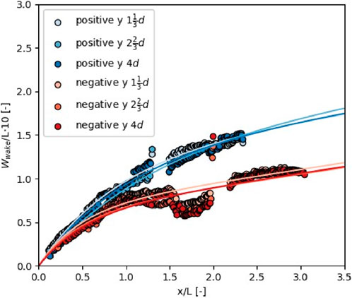
Figure 12. Horizontal wake spreading over the depth for the negative and positive y-side, including an exponential fit where the data are averaged over time with 22.5°.

In a subsequent step, the data of three water depths are combined, and the dependency of W_wake on the array size and its orientation is analyzed. The analysis of the simulations for various orientations showed that the wake width is likely to depend on the corner length (L_c) of the array, next to the angle of attack (AoA) of the current. The dependency on the angle of attack becomes apparent when, after normalizing the results by L_c, the results for the positive and negative y-domain for the orientation of 45° are on top of each other, while for 22.5° and 67.5°, it differs between the two sides of the y-domain. However, the results of both orientations of 22.5° and 67.5° matched when the angle of attack of a side was the same. The angle of attack of one side of the y-domain has a 45° difference with the angle of attack of the opposite side.

The resulting data points indicating the wake width are normalized by an ad hoc Equation 5 for the correction factor c. This factor depends on the angle of attack in radians and becomes higher than 1 when the angle of attack of one side is moderate (22.5°).

$c=\left\{\begin{array}{ll}\frac{3}{8}\pi & \mathrm{if}\hspace{0.17em}\mathit{AoA}=22.5°\\ 1\hfill & \mathrm{otherwise}.\end{array}\right.(5)$

The data are normalized by c and L_c and combined in Figures 13A, B. The data fit for the asymmetric cases in Figure 13A (rotation α between 0° and 90°) is shown to be exponential, while for the symmetric cases, as shown in Figure 13B (rotation α equal to 0° or 90°), the fit is linear. The final fit for all data combined is illustrated as a black dashed line and has the form W_wake = a ·(1 − exp (−b · x)) + f · x.

Figure 13

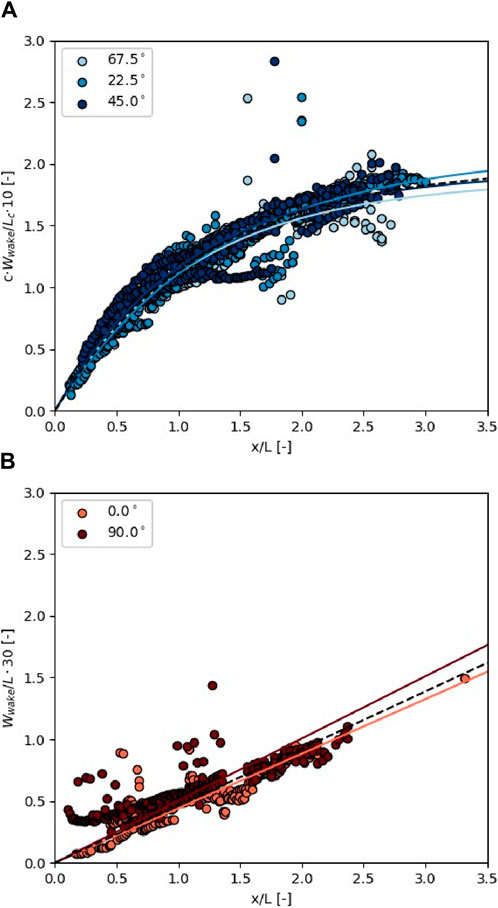
Figure 13. (A) Asymmetric cases. (B) Symmetric cases. Fit of the horizontal wake spreading for different rotation angles α.

Based on the limited data, a formulation is made for the wake width W_wake given in Equation 6:

$W_{wake}=\underset{\text{Asymmetric}}{\underbrace{\frac{39}{200}\frac{s\cdot L_c}{c}\left(1-e^{-\frac{17x}{20L}}\right)}}+\underset{\text{symmetric}}{\underbrace{\frac{23}{1500}}}x(6)$

where s (symmetry) is only equal to 1 when the array is rotated (rotation α between 0° and 90°). The distance x and L are in m.

The standard deviation of every coefficient is determined. For the linear coefficient (23/1500) of the symmetric part, the deviation is below 1%. For the remaining two coefficients of the asymmetric part, the standard deviation is below 2%.

The asymmetry of the array can result in the total wake width of 1.25 (67.5°) and 1.3 (22.5°) times the frontal width W_y. On top of that, the wake width increases linearly with 15 m after a kilometer, independent of W_y and the orientation. Notably, the linear increase in W_wake with distance x makes it rather conservative, whereas in reality, it is expected that the wake diffuses.

Similarly, for the increase in the ambient current with a factor of 2 (Re_L = 3.66e7), a fit for a rotation of 67.5° resulted in an increase in coefficient 39/200 with 15%. The exponential coefficient 17/20 becomes 20% less dominant.

4 Discussion

4.1 Large-scale application and co-location

In order to limit the space needed for offshore energy generation, offshore solar is foreseen to be co-located within offshore wind farms. This co-location will place solar arrays between the offshore wind turbines, providing three key benefits: 1) offshore solar farms, with a power density of 150–200 MW/km² compared to 5–10 MW/km² for offshore wind, fit well within the spaces of approximately 1.5–2.5 km between (modern) wind turbines; 2) solar and wind energy complement each other (Golroodbari et al., 2021; Lo’pez et al., 2020), with wind peaking in winter and harsh weather and solar in summer and calm conditions; and 3) multi-use of sea space benefits marine spatial planning, leaving more areas available for nature, recreation, fishing, and other blue economy activities.

As co-location of (bottom-fixed) wind turbines and floating solar arrays might become abundant in the future in shallow shelf seas like the North Sea, the hydrodynamic conditions in the near and far-field, both in the horizontal and vertical direction, as changed by the many bottom-fixed turbines (Sumer and Fredsøe, 2006; Schultze et al., 2020; Christiansen et al., 2023), will also affect the flow patterns that surround the floating solar farms. The flow approaching the solar arrays will be more turbulent and less consistent as assumed within this study. This could affect the wake development around the offshore solar array, but as the distance between the offshore wind turbines and the offshore solar arrays is probably equal to or larger than the wake length, this effect is likely limited.

Offshore solar is foreseen to be employed on a large scale, where arrays span up to multiple kilometers. However, in this study, we focused on a smaller array to achieve realistic computational costs, while still maintaining grid accuracy near the array. It is unclear whether or how the results of this study can be transferred to larger scales since the investigations do not cover enough scale variations to provide a stable data basis. Flow phenomena larger than the wide 3D domain are not included.

4.2 Effect of marine growth

In the presented simulations, the floaters are parameterized as rough floaters with a limited submerged depth. Herein, the roughness is approximated by consistent roughness elements, characterized by Nikuradse’s equivalent sand roughness (Nikuradse, 1933; Schlichting and Gersten, 2016). However, while this approximation is reasonable for the initial phase when the floaters and interconnectors have just been deployed, over time, the floaters will get colonized by marine biota, which introduces an increased roughness to the surface, likely affecting the hydrodynamic behavior. This is mentioned as well in the Supplementary Material.

Marine growth tends to occur in distinct layers over the water column (Degraer et al., 2012; Krone et al., 2013). In temperate climates, such as the North Sea, offshore infrastructure for oil and gas and wind turbines in the upper 1–6 m tend to be dominated by bivalves. As the floaters are restricted to the surface, these communities are expected to dominate on offshore solar arrays (Mavraki et al., 2023). The rigid shells of bivalves impact the properties of the near-surface boundary layer (Green et al., 1998). The turbulence in the vicinity of the floater surface is not only influenced by the roughness caused by the shell structures but can also be modified by the direct input of turbulence by the interaction of the bivalve feeding currents with the boundary layer flow (Van Duren et al., 2006).

The accumulation of marine growth will impact drag and add to the loads of the offshore solar array, similar to the way fouling organisms influence drag on a ship’s hull (Catipovic’ et al., 2022; Song et al., 2020). To what extent biota on the offshore solar array will impact the hydrodynamic wake remains to be seen, but based on the influence of biofouling on wake forms behind ships, we expect this effect to be limited (Newman, 2018).

4.3 Representation of local hydrodynamics

In our study, we only considered the interaction between the offshore solar array and the tidal current. This means we neglected not only other environmental processes such as waves and wind shear but also the movability of the solar array. In reality, these will also affect hydrodynamics around the array. The wave interaction will likely contribute to turbulent mixing, resulting in a decrease in wake size (Al-Yacouby et al., 2020; Schreier and Jacobi, 2021; Xu and Wellens, 2022). The same could happen due to the wind (Lee et al., 2021). The dynamic interaction is expected to mitigate the wake dimensions due to increased dissipation. The effect of the movability of the floating solar array and the influence of waves on the hydrodynamic wake development should be part of future investigations. Furthermore, an increase in marine growth can substantially affect the boundary layer thickness beneath the array and warrants further investigation in the future.

Furthermore, we assumed a uniform current over depth. This was based on a preliminary assessment of the influence of the seabed at a depth of $213\frac{1}{3}$d, which showed that it had a small influence (1.5%) on the flow velocities near the floaters. This small influence makes the assumption of using a uniform current valid.

When designing the grid, we opted for a somewhat coarser grid in the downstream area of the array. Although the grid is sufficiently fine to resolve at least 80% of the total turbulent kinetic energy, the grid cell sizes are in a similar order as the turbulent eddy size. In turn, this may reduce vortex stretching. Simulations with TUDFLOW3D, which had a finer grid resolution in the downstream area, showed that the results are similar. Thus, the grid design in the downstream area appeared to have a limited effect on our results.

5 Conclusions

Offshore solar is seen as a promising technology for renewable energy generation. The impacts of offshore solar on the surrounding environment are not fully understood yet, including how the floating structures might affect local hydrodynamics.

In this study, we aimed to quantify the dimensions of a hydrodynamic wake generated by an offshore solar array. We performed large eddy simulations (LES) using OpenFOAM, for an array in a stationary configuration, interacting with a tidal current. The hydrodynamic wake originates from flow-shedding effects and the development of a boundary layer. Simulations were run for five rotations of the array, three different array lengths, and two different ambient currents. The wake is analyzed in two stages: beneath the array and behind the array.

Beneath the array, the development of the boundary layer depends on the floater size and the gap between floaters. Flow separation occurs at these gaps, with a shedding of approximately 0.08. When the gaps between the floaters are of a similar length as the boundary layer thickness, they will likely prevent the gradual increase in the boundary layer thickness. In this case, the total array cannot be considered a thin plate. The boundary layer thickness for the given configuration, with gaps, is 33% lower than theoretical formulations for a turbulent flow along a thin plate. The size of the turbulent features due to flow separation largely depends on the angle of attack of the current and the horizontal dimensions of the floater and can increase the local depth with a factor larger than 20 times the submerged depth.

Behind the array, we consider the three wake dimensions: length, depth, and width. Wake lengths of 10 times the array length are likely and influenced by factors such as array length, current magnitude and, on top of that, the gaps in between the floaters. The dependency on the current magnitude is most prominent. The presence of gaps in the order of the boundary layer thickness reduces the dependency of the vertical wake dimensions on the array length and current.

Similarly, the wake depth showed fewer dependencies and is typically of a lower order of magnitude than the wake length and width, but up to 17 times the submerged depth of the array. The gaps between the floaters reduce the wake depth.

Wake width highly depends on both array orientation and horizontal dimensions. The local wake width has an initial size equal to the projected frontal width of the array. When the array is aligned with the current, wake width is relatively confined and increases linearly in distance. Rotating the array results in an additional exponential increase in the wake width of up to 30% more than the projected array width. The change in the wake width over depth is negligible compared to the total dimensions.

Non-dimensional formulations for wake dimensions have been derived based on our simulations. When scaling up offshore solar, these can be used as an estimate for possible hydrodynamic wakes. In turn, these insights can eventually be used to assess the impact of large-scale offshore solar on physical and biotic processes in the marine environment.

Data availability statement

The raw data supporting the conclusions of this article will be made available by the authors, without undue reservation.

Author contributions

MV: conceptualization, formal analysis, investigation, methodology, visualization, and writing–original draft. DP: conceptualization, methodology, and writing–review and editing. EH: conceptualization, project administration, and writing–review and editing. LD: investigation, methodology, and writing–review and editing.

Funding

The authors declare that financial support was received for the research, authorship, and/or publication of this article. The authors declare financial support was received for the research, authorship, and/or publication of this article. The research was carried out in the Sense-Hub project, which was funded by RVO (Rijksdienst voor Ondernemend Nederland) through grant number MOOI622002. Funding for writing this article was received from the Deltares internal strategic research budget, as provided to Deltares by the Dutch Ministry of Economic Affairs and Climate.

Acknowledgments

The authors would like to thank Oceans of Energy for the collaboration and fruitful discussions when setting up and carrying out this research. They would also like to thank Brigitte Vlaswinkel and Luca van Duren for their review of the draft manuscript. The other partners in the Sense-Hub project are acknowledged for their interest in our work and constructive feedback.

Conflict of interest

The authors declare that the research was conducted in the absence of any commercial or financial relationships that could be construed as a potential conflict of interest.

Publisher’s note

All claims expressed in this article are solely those of the authors and do not necessarily represent those of their affiliated organizations, or those of the publisher, the editors, and the reviewers. Any product that may be evaluated in this article, or claim that may be made by its manufacturer, is not guaranteed or endorsed by the publisher.

Supplementary material

The Supplementary Material for this article can be found online at: https://www.frontiersin.org/articles/10.3389/fenrg.2024.1434356/full#supplementary-material

References

Al-Yacouby, A., Halim, E. R. B. A., and Liew, M. (2020). “Hydrodynamic analysis of floating offshore solar farms subjected to regular waves,” in Advances in manufacturing engineering: selected articles from ICMMPE 2019 (Springer), 375–390.

CrossRef Full Text | Google Scholar

Benjamins, S., Williamson, B., Billing, S.-L., Yuan, Z., Collu, M., Fox, C., et al. (2024). Potential environmental impacts of floating solar photovoltaic systems. Renew. Sustain. Energy Rev. 199, 114463. doi:10.1016/j.rser.2024.114463

CrossRef Full Text | Google Scholar

Catipovic’, I., Alujevic’, N., Smoljan, D., and Mikulic’, A. (2022). “A review on marine applications of solar photovoltaic systems,” in 15th international symposium on practical design of ships and other floating structures-PRADS 2022, 1804–1820.

Google Scholar

Chen, H., and Christensen, E. D. (2018). Simulating the hydrodynamic response of a floater–net system in current and waves. J. Fluids Struct. 79, 50–75. doi:10.1016/j.jfluidstructs.2018.01.010

CrossRef Full Text | Google Scholar

Christiansen, N., Carpenter, J. R., Daewel, U., Suzuki, N., and Schrum, C. (2023). The large-scale impact of anthropogenic mixing by offshore wind turbine foundations in the shallow north sea. Front. Mar. Sci. 10, 1178330. doi:10.3389/fmars.2023.1178330

CrossRef Full Text | Google Scholar

Daewel, U., Akhtar, N., Christiansen, N., and Schrum, C. (2022). Offshore wind farms are projected to impact primary production and bottom water deoxygenation in the north sea. Commun. Earth and Environ. 3, 292. doi:10.1038/s43247-022-00625-0

CrossRef Full Text | Google Scholar

Dataset OpenCFD (2004). Openfoam programmers guide.

Google Scholar

Degraer, S., Brabant, R., and Rumes, B. (2012). Offshore wind farms in the Belgian part of the North Sea: heading for an understanding of environmental impacts. Royal Belgian Institute of Natural Sciences.

Google Scholar

De Wit, L. (2015). 3d cfd modelling of overflow dredging plumes.

Google Scholar

De Wit, L., Keetels, G., and Van Rhee, C. (2015). Turbulent interaction of a buoyant jet with crossflow. J. Hydraulic Eng. 140. doi:10.1061/(asce)hy.1943-7900.0000935

CrossRef Full Text | Google Scholar

De Wit, L., Plenker, D., and Broekema, Y. (2023). 3d cfd les process-based scour simulations with morphological acceleration.

Google Scholar

de Wit, L., and van Rhee, C. (2014). Testing an improved artificial viscosity advection scheme to minimise wiggles in large eddy simulation of buoyant jet in crossflow. Flow, Turbul. Combust. 92, 699–730. doi:10.1007/s10494-013-9517-1

CrossRef Full Text | Google Scholar

Dey, S. (2014). Fluvial hydrodynamics. Berlin, Heidelberg: Springer Berlin Heidelberg.

Google Scholar

D’ıaz-Ojeda, H. R., Huera-Huarte, F., and Gonza’lez-Gutie’rrez, L. M. (2019). Hydrodynamics of a rigid stationary flat plate in cross-flow near the free surface. Phys. Fluids 31. doi:10.1063/1.5111525

CrossRef Full Text | Google Scholar

Garcia, M., and Parker, G. (1993). Experiments on the entrainment of sediment into suspension by a dense bottom current. J. Geophys. Res. Oceans 98, 4793–4807. doi:10.1029/92jc02404

CrossRef Full Text | Google Scholar

Golroodbari, S., Vaartjes, D., Meit, J., van Hoeken, A., Eberveld, M., Jonker, H., et al. (2021). Pooling the cable: a techno-economic feasibility study of integrating offshore floating photovoltaic solar technology within an offshore wind park. Sol. Energy 219, 65–74. Special Issue on Floating Solar: beyond the. doi:10.1016/j.solener.2020.12.062

CrossRef Full Text | Google Scholar

Green, M. O., Hewitt, J. E., and Thrush, S. F. (1998). Seabed drag coefficient over natural beds of horse mussels (atrina zelandica). J. Mar. Res. 56, 613–637. doi:10.1357/002224098765213603

CrossRef Full Text | Google Scholar

Group, W. B., and Esmap, SERIS (2019). Where sun meets water Floating solar market report, 2. Washington, D.C.: World Bank Group.

Google Scholar

Hemmati, A., Wood, D. H., and Martinuzzi, R. J. (2017). “Evolution of vortex formation in the wake of thin flat plates with different aspect-ratios,” in Progress in turbulence VII: Proceedings of the iTi Conference in turbulence 2016 (Springer), 227–232.

CrossRef Full Text | Google Scholar

Hooper, T., Armstrong, A., and Vlaswinkel, B. (2021). Environmental impacts and benefits of marine floating solar. Sol. Energy 219, 11–14. doi:10.1016/j.solener.2020.10.010

CrossRef Full Text | Google Scholar

Karniadakis, G. E., and Triantafyllou, G. S. (1992). Three-dimensional dynamics and transition to turbulence in the wake of bluff objects. J. fluid Mech. 238, 1–30. doi:10.1017/s0022112092001617

CrossRef Full Text | Google Scholar

Karpouzoglou, T., Vlaswinkel, B., and Van Der Molen, J. (2020). Effects of large-scale floating (solar photovoltaic) platforms on hydrodynamics and primary production in a coastal sea from a water column model. Ocean Sci. 16, 195–208. doi:10.5194/os-16-195-2020

CrossRef Full Text | Google Scholar

Kim, M., Lim, J., Kim, S., Jee, S., Park, J., and Park, D. (2019). Large-eddy simulation with parabolized stability equations for turbulent transition using openfoam. Comput. and Fluids 189, 108–117. doi:10.1016/j.compfluid.2019.04.010

CrossRef Full Text | Google Scholar

Kim, W.-W., and Menon, S. (1995). “A new dynamic one-equation subgrid-scale model for large eddy simulations,” in 33rd aerospace sciences meeting and exhibit, 356.

CrossRef Full Text | Google Scholar

Knisely, C. W. (1990). Strouhal numbers of rectangular cylinders at incidence: a review and new data. J. fluids Struct. 4, 371–393. doi:10.1016/0889-9746(90)90137-t

CrossRef Full Text | Google Scholar

Koundouri, P., Manoussi, V., and Papadaki, L. (2021). Introduction to the oceans of tomorrow: the transition to sustainability. Ocean Tomorrow Transition Sustain. 2, 1–24. doi:10.1007/978-3-030-56847-4_1

CrossRef Full Text | Google Scholar

Krone, R., Gutow, L., Joschko, T. J., and Schro¨ der, A. (2013). Epifauna dynamics at an offshore foundation–implications of future wind power farming in the north sea. Mar. Environ. Res. 85, 1–12. doi:10.1016/j.marenvres.2012.12.004

PubMed Abstract | CrossRef Full Text | Google Scholar

Kumar, V., Shrivastava, R., and Untawale, S. (2015). Solar energy: review of potential green and clean energy for coastal and offshore applications. Aquat. Procedia 4, 473–480. doi:10.1016/j.aqpro.2015.02.062

CrossRef Full Text | Google Scholar

Lee, G.-H., Choi, J.-W., Kim, J., Seo, J.-H., and Ha, H. (2021). Numerical simulations of wind loading on the floating photovoltaic systems. J. Vis. 24, 471–484. doi:10.1007/s12650-020-00725-z

CrossRef Full Text | Google Scholar

López, M., Rodríguez, N., and Iglesias, G. (2020). Combined floating offshore wind and solar pv. J. Mar. Sci. Eng. 8, 576. doi:10.3390/jmse8080576

CrossRef Full Text | Google Scholar

Mavraki, N., Bos, O. G., Vlaswinkel, B. M., Roos, P., de Groot, W., van der Weide, B., et al. (2023). Fouling community composition on a pilot floating solar-energy installation in the coastal Dutch north sea. Front. Mar. Sci. 10. doi:10.3389/fmars.2023.1223766

CrossRef Full Text | Google Scholar

Miles, J., Martin, T., and Goddard, L. (2017). Current and wave effects around windfarm monopile foundations. Coast. Eng. 121, 167–178. doi:10.1016/j.coastaleng.2017.01.003

CrossRef Full Text | Google Scholar

Nassar, W. M., Anaya-Lara, O., Ahmed, K. H., Campos-Gaona, D., and Elgenedy, M. (2020). Assessment of multi-use offshore platforms: structure classification and design challenges. Sustainability 12, 1860. doi:10.3390/su12051860

CrossRef Full Text | Google Scholar

Newman, J. N. (2018). Marine hydrodynamics. The MIT press.

Google Scholar

Nicoud, F., and Ducros, F. (1999). Subgrid-scale stress modelling based on the square of the velocity gradient tensor. Flow, Turbul. Combust. 62, 183–200. doi:10.1023/a:1009995426001

CrossRef Full Text | Google Scholar

Nikuradse, J. (1933). Stro¨ mungsgesetze in rauhen Rohren. 361 Verein deutscher Ingenieure - Forschungsheft.

Google Scholar

Oliveira-Pinto, S., and Stokkermans, J. (2020). Marine floating solar plants: an overview of potential, challenges and feasibility. Proc. Institution Civ. Engineers-Maritime Eng. 173, 120–135. doi:10.1680/jmaen.2020.10

CrossRef Full Text | Google Scholar

Renewables Now (2018). Renewables 2018: Global Status Report, Renewable Energy Policy Network for the 21st Century. Paris, France: REN21 Publication.

Google Scholar

Rostami, A. B., Mobasheramini, M., and Fernandes, A. C. (2019). Strouhal number of flat and flapped plates at moderate Reynolds number and different angles of attack: experimental data. Acta Mech. 230, 333–349. doi:10.1007/s00707-018-2292-2

CrossRef Full Text | Google Scholar

Ruzzo, C., Muggiasca, S., Malara, G., Taruffi, F., Belloli, M., Collu, M., et al. (2021). Scaling strategies for multi-purpose floating structures physical modeling: state of art and new perspectives. Appl. Ocean Res. 108, 102487. doi:10.1016/j.apor.2020.102487

CrossRef Full Text | Google Scholar

Sanjay, S., Sundararaj, S., and Thiagarajan, K. B. (2019). Numerical simulation of flat plate boundary layer transition using openfoam®. In AIP conference proceedings AIP Publishing, vol. 2112

CrossRef Full Text | Google Scholar

Schlichting, H., and Gersten, K. (1979). Boundary-layer theory 7th ed. New York, NY: McGraw-hill.

Google Scholar

Schreier, S., and Jacobi, G. (2021). Experimental investigation of wave interaction with a thin floating sheet. Int. J. Offshore Polar Eng. 31, 435–444. doi:10.17736/ijope.2021.mk76

CrossRef Full Text | Google Scholar

Schultze, L., Merckelbach, L., Horstmann, J., Raasch, S., and Carpenter, J. (2020). Increased mixing and turbulence in the wake of offshore wind farm foundations. J. Geophys. Res. Oceans 125, e2019JC015858. doi:10.1029/2019jc015858

CrossRef Full Text | Google Scholar

Song, J., Kim, J., Lee, J., Kim, S., and Chung, W. (2022). Dynamic response of multiconnected floating solar panel systems with vertical cylinders. J. Mar. Sci. Eng. 10, 189. doi:10.3390/jmse10020189

CrossRef Full Text | Google Scholar

Song, S., Demirel, Y. K., Muscat-Fenech, C. D. M., Tezdogan, T., and Atlar, M. (2020). Fouling effect on the resistance of different ship types. Ocean. Eng. 216, 107736. doi:10.1016/j.oceaneng.2020.107736

CrossRef Full Text | Google Scholar

Sumer, B. M., and Fredsøe, J. (2006). Hydrodynamics around cylindrical structures, Advanced series on ocean engineering (Singapore and London: World Scientific Publishing), revised ed. edn.

Google Scholar

Van Duren, L. A., Herman, P. M., Sandee, A. J., and Heip, C. H. (2006). Effects of mussel filtering activity on boundary layer structure. J. Sea Res. 55, 3–14. doi:10.1016/j.seares.2005.08.001

CrossRef Full Text | Google Scholar

Vlaswinkel, B., Roos, P., and Nelissen, M. (2023). Environmental observations at the first offshore solar farm in the north sea. Sustainability 15, 6533. doi:10.3390/su15086533

CrossRef Full Text | Google Scholar

Xu, P., and Wellens, P. R. (2022). Fully nonlinear hydroelastic modeling and analytic solution of large-scale floating photovoltaics in waves. J. Fluids Struct. 109, 103446. doi:10.1016/j.jfluidstructs.2021.103446

CrossRef Full Text | Google Scholar

Zheng, X., Zheng, H., Lei, Y., Li, Y., and Li, W. (2020). An offshore floating wind–solar–aquaculture system: concept design and extreme response in survival conditions. Energies 13, 604. doi:10.3390/en13030604

CrossRef Full Text | Google Scholar