Abstract
Energy system optimization is needed for optimal sustainable net-zero electricity (NZE) mix even at regional/local scales because of the energy storage needs for addressing the intermittency of renewable energy supply. This study presents a novel regional/local energy planning model for optimum sustainable NZE mix under spatiotemporal climate/meteorological and electrical load demand constraints. A generic robust non-linear constrained mathematical programming (NLP) algorithm has been developed for energy system optimization; it minimizes the levelized cost and greenhouse gas emissions while maximizing reliability against stored energy discharge analysis (RADA). Reliability, defined as the ratio of excess stored renewable power discharge to unmet load demand, is a measure of the extent of unmet load demand met by the excess stored renewable power. Coupled with the NLP, the RADA and energy storage evaluations are used to determine the seasonal energy storage (SES) conditions and realistic renewable proportions for NZE. The significance of the proposed framework lies in determining the maximum hours of viable electrical energy storage beyond which the reliability enhancement is infinitesimal. The significant observations of this work include 96 h of maximum viable electrical energy storage beyond which the reliability enhancement is infinitesimal. While this observation is robust based on previous reports for the case of the United States, a realistic NZE mix for Southern United Kingdom is obtained as follows. Direct wind and solar sources can meet 63%, 62%, and 55% of the electricity demands in the southwest, Greater London, and southeast regions of the United Kingdom, respectively; further, battery energy storage systems can increase the renewable proportions by 21%, 22%, and 13% in these three regions. The unmet demands can be met by renewable electricity through SES. Compressed air energy storage (CAES) and pumped hydro storage offer viable SES. Following these, natural gas with carbon capture and storage (CCS), bioenergy, and hydrogen SES are the choices based on increasing cost per lifecycle climate impact potential to meet the electricity demands.
1 Introduction
The complex intrinsic interactive nature of a net-zero electricity (NZE) system considering renewable, bioenergy, and carbon capture and storage (CCS) as well as energy storage (hourly and seasonal) and transmission systems entails whole-system optimization of the distributed/centralized design choices based on a myriad of options. Such optimization problems are pervasive in whole-energy and power systems, energy storage design, scheduling, control strategies, climate data analyses for geophysical constraints on wind and solar power reliability, behavior change interventions for demand-side management, and low-carbon NZE for local/regional to national and planetary scales. Interconnecting these problems through optimization for robust long-term sustainable design is a complex and high-dimensional post-COP26 challenge.
Directly dispatchable wind and solar power generation systems have the least lifecycle greenhouse gas emissions (GHGs), making them leading choices for NZE systems (Sadhukhan, 2021). Their lower costs compared to other renewable options, hydropower and geothermal sources, carbon-neutral bioenergy, natural gas combined cycle or power plants with CCS (gas with CCS), and nuclear power mark them as minimal-cost choices for NZE systems (Bogdanov et al., 2019; Bogdanov et al., 2021). Further, solar and wind power costs are expected to decline at staggering rates than other renewable and low-carbon energy options owing to their learning curve effects. Most studies on power or energy system analyses suggest high wind and solar proportions in the NZE mix (Lund and Vad Mathiesen, 2009; Lu et al., 2021). NZE requires carbonless fossil-independent renewable energy generation systems. Hence, wind and solar power generation hold considerable proportions in the NZE mix despite their interannual variabilities (Perez-Arriaga and Batlle, 2012; Zhou et al., 2018).
Realistic models with geophysical constraints influencing the availability of wind speed and solar radiation underscore the need for several weeks’ worth of energy storage (Shaner et al., 2018; Houssainy and Livingood, 2021; Sadhukhan et al., 2022). Pumped hydro storage (PHS), compressed air energy storage (CAES), and hydrogen energy storage (HES) systems constitute the seasonal energy storage (SES) category. GHGs accounting for battery energy storage systems (BESSs) (Sadhukhan and Christensen, 2021) are aligned with economic observations compelling readily available dispatchable power options that are more attractive than extra wind and solar capacities with energy storage (Bogdanov et al., 2019; Bogdanov et al., 2021). Therefore, robust energy storage evaluations are essential for local and regional authorities planning to deploy wind and solar power heavily for NZE to avoid unintended costs or GHG consequences. Technology-driven studies have considered state-of-the-art options that provide a few hours of battery energy storage (Yao et al., 2011; Al-Ghussain et al., 2018), while climate-driven studies have suggested several weeks of energy storage requirements as the direction for future developments (Lund and Vad Mathiesen, 2009; Shaner et al., 2018; Bakhtvar et al., 2021). When the stored electricity dispatch time exceeds a few hours to a few weeks, seasonal storage is required in the form of CAES, PHS, and HES. After a few hours of battery energy storage, the unmet load is often met by carbon-efficient dispatchable power, bioenergy, and gas with CCS rather than renewable SES because of the higher cost implications of the SES options (Denholm and Margolis, 2007; Yousif et al., 2019; Dowling et al., 2020). However, the sequence in which the various energy storage systems should be deployed to enhance NZE should be governed by a holistic systemic-optimization-based analysis, which is not available in existing works (Denholm and Margolis, 2007; Yousif et al., 2019; Dowling et al., 2020).
Holistic, systemic, and systematic optimization-based analyses are required to objectively inform not only the least-cost but also minimum-GHG NZE mix. Some of the research questions in the planning model for the NZE that remain unresolved are as follows: 1) Is it practical to meet all electricity demands through renewable self-generation, especially wind and solar types, with minimal cost and GHG that may need seasonal storage? 2) What is the optimal energy storage duration for maximum reliability, which is the extent of excess renewable power utilization in meeting the unmet load demand, beyond which the increases in reliability are infinitesimally small? These questions underscore the need for a powerful robust whole-system optimization-based framework for multiscale energy system planning, which defines the aims of this study. Hence, this study provides a novel framework for optimal energy storage choices and duration for maximum-reliability renewable NZE.
There are a few available optimization models for energy system planning targeted to achieve large-scale NZE. The principal methodologies include linear constrained optimization studies (Dorfner, 2016; Brown et al., 2018) and statistical analyses (Shaner et al., 2018; Tong et al., 2021) that evaluate the minimum-cost electricity mix from local (Weber and Shah, 2011; Gil et al., 2021) to national or regional (Brouwer et al., 2016; Zeyringer et al., 2018) to global (Tong et al., 2021) scales. These approaches span annual (Sameti and Haghighat, 2018) to multiyear (Zhang, 2014) and multidecade (Shaner et al., 2018) considerations, with resolutions of a few minutes (Zhang, 2014; Safaei and Keith, 2015) to hourly (Monforti et al., 2014). A few studies explicitly consider energy storage conditions when defining the optimization constraints (Khalid et al., 2016; Watson et al., 2017; Anoune et al., 2018; Mazzeo et al., 2018). Energy system planning models using deterministic mathematical programming, particularly linear or mixed-integer linear programming, optimize the quantities of interest, installed capacities of the system components (Aboumahboub et al., 2010; Prebeg et al., 2016), energy mixes (Weijermars et al., 2012; Augutis et al., 2015; Thangavelu et al., 2015; Wierzbowski et al., 2016; Nirbheram et al., 2023), wind and solar penetrations in the energy mix (Franco and Salza, 2011; Nikolakakis and Fthenakis, 2011; Zappa and van den Broek, 2018; Ullah et al., 2021), storage system characterizations (Terlouw et al., 2019; Rahbari et al., 2021), meteorological data analyses (Firatoglu and Yesilata, 2004; Jane et al., 2020), as well as supply-side and demand-side managements (Atzeni et al., 2012; Tan et al., 2016).
On the contrary, power systems engineering with lower dimensionality at the distributed/mini-grid scale tends to use stochastic optimization methods (Niaei et al., 2022; Sadeghi et al., 2022). Another review based on 550 articles on solar and wind electricity systems reported that the most frequently used optimization algorithms were the particle swarm optimization and genetic algorithms (Mazzeo et al., 2021a). Moreover, artificial neural networks are trending in the application of artificial intelligence for sizing and simulating energy systems, including energy storage (Mazzeo et al., 2021b). However, it is noted that the high-dimensional optimization model presented in this article is meant for large-scale energy planning (national or regional level), where stochastic optimization has not been applied yet. A handful of studies are also available on the detailed evaluations of energy storage options (Razmi and Janbaz, 2020; Alirahmi et al., 2021; Li et al., 2023). Such detailed models are not needed in large-scale high-level planning. Although the methodological framework presented herein is generic and includes further storage options, such as thermal energy storage, the case study only includes BESS with CAES, PHS, and HES as the SES options to enhance the proportion of renewable electricity in the mix.
The optimization formulations for large-scale high-dimensional energy system planning for NZE comprise constraints such as the mathematical models of the components, bounds on their capacities, climatological and demand time series, and objective functions to minimize the total costs (Bogdanov et al., 2021; Sadhukhan et al., 2022). A significant constraint in the optimization model formulation is the energy balance at the time resolution. The smaller the time resolution step (e.g., hourly) and longer the total duration of the supply–demand time series (e.g., multidecade) considered during optimization, the less likely it is to achieve convergence and a robust reproducible solution. To overcome these obstacles, large-scale high-dimensional energy system planning optimization algorithms often consider linear and mixed-integer linear programming (Bogdanov et al., 2021). Our earlier work involved non-linear constrained mathematical programming (NLP) to optimize the NZE system (Sadhukhan et al., 2022); however, this work only considered BESSs for energy storage. The present work is a pioneering effort at incorporating SES in an NLP-based optimization analysis for a large-scale high-dimensional energy system planning model. Herein, a novel approach coupling NLP, reliability against stored energy discharge analysis (RADA), and energy storage evaluations is developed to maximize the renewables in the NZE mix for minimum cost and GHG emissions under high-resolution spatiotemporal climate meteorological and electrical load demand constraints. The remainder of this paper is structured as follows. The methodologies discuss the NLP, RADA, and energy storage system models. Then, a case study focusing on an energy-intensive region (South of the United Kingdom) is used to demonstrate the efficacy of the framework. The results, discussion, and conclusions of the study are provided thereafter.
2 Materials and methods
The NLP model minimizes the total cost accounting for all new investment, variable, fixed, resource, GHG, upgrading, and decommissioning costs (Sadhukhan et al., 2022). The optimization problem can be defined as a multiobjective optimization problem, with cost and GHG minimization as the two objectives. However, the cost and GHG minimization objectives are not in conflict with each other because the two primary renewable technologies (wind and solar) are the cheapest and minimal-GHG options among all plausible systems for NZE. Considering the GHG cost in the optimization objective function allows choosing the minimum-cost and minimum-GHG options as the optimal solution. It is noted that GHG implies that the lifecycle global warming potential is considered in terms of the carbon dioxide equivalent of cradle-to-grave of each technological system under consideration. The lifecycle stages of the technologies for the lifecycle global warming potential, i.e., GHG in this work, include the operation phases of the technologies. Consistent literature sources have been used to collect the GHG impact data on the technologies. For example, literature based on Ecoinvent as the lifecycle inventory data source and IPCC methodology for the lifecycle global warming potential impact calculations and authoritative reports are considered as trusted sources. These sources have a global consensus and no conflicts in the systemic choices for the technological GHG impact calculations. The optimization model thus remains valid even when the input data are changed. The storage options are relevant for electrical energy storage. The complete set of NLP model equations and nomenclatures are shown in the Supplementary Material. Figure 1 illustrates a whole-energy system planning model comprising NLP interacting with RADA and energy storage evaluations for a minimum-cost GHG and maximum-reliability solution obtained from the weather (climatology) and demand time series as well as technical, environmental, and economic parameter inputs.
FIGURE 1

The whole energy system planning model.
The multiscale mathematical models of bioenergy and renewable energy systems (wind, solar, hydro, and geothermal) from hourly weather and design configuration data are calibrated across the temporal and spatial scales. The interdisciplinary data platforms seek climatology, design configuration, technical, cost, and environmental parameters along with the load demand constraints as inputs. Models are developed for renewable generation as well as supply chain logistics including storage, bioenergy, and gas CCS systems. Mathematical programming is used to calculate the optimal capacities for installing various technologies for a given objective, e.g., minimum-cost GHG. The multiobjective optimization technique offers Pareto solutions, i.e., optimal proportions of technologies for the best tradeoffs between the objectives. However, the cost and GHG minimization objectives are aligned in the case of NZE. Thus, by accounting for the GHG costs, the optimization problem can be formulated and solved as a single-objective NLP to minimize the overall cost.
The objective of this work is minimization of a complete NZE system’s total cost over a given time scale, e.g., annual or decadal or multidecadal. The total cost comprises the weighted average capital, fixed, variable, resource, pollution including GHG, upgrading, and decommissioning costs of the individual components in the entire energy system within the given time scale. The cost parameters, such as unit costs of the processes, can vary over time and across the spatial scale. Such spatiotemporal variations in the parameters can be captured via linear regression equations, leading to non-linear equations. The capacity-factor-based wind and solar power generations are also non-linear equations. These non-linear correlation constraints make the optimization problem an NLP consideration. The other constraints are the upper and lower bounds of each unit capacity in the entire energy system and energy balance equations at each of the lowest time resolutions. Detailed equations and explanations are provided in the Supplementary Material. Here, the wind and solar power generations as well s energy balance equations are discussed, which influence the energy storage choices.
Wind and solar power generations are calculated from the weather data at the individual smallest spatiotemporal resolutions via their capacity factors. The capacity factors are defined as the extents of installed power utilizations dependent on the availabilities of wind speed and solar radiation (provided by climatology), as shown in Eqs (1a, 1b, 2).Here, is the power output of a wind or solar system and is calculated from the wind speed () and solar radiation (), as shown in Eqs (1a, 1b, 2), respectively (Sadhukhan et al., 2022). Eq. (1a) shows of a wind turbine as a function of the density of air (), area swept by the turbine blades (), wind speed (), and capacity factor of the wind turbine (). Eq. (1b) is valid for a wind speed of 4–25 m/s and shows the dependency of the capacity factor on ; here, , , , and are the cut-in and cut-out speeds, scale parameters, and shape parameters of the wind turbine, respectively.
Equation (2) shows that is the power output of the solar system, which is the product of its area (), solar radiation (), and capacity factor (); here, is scaled between 0.025 and 0.21 for the UK-based case study based on annual variations over the past 5 years (Sadhukhan et al., 2022) to represent the minimum solar radiation () and maximum solar radiation ().
The energy supply comprises the energy stored in the previous time step and energy generation by the operational processes in the present time step () (right-hand side of Eq. (3a)). The energy demand, transmission loss, and energy stored are added to obtain the total energy output [left-hand side of Eq. 3a] to balance the energy input at the given time step. Eq. (3b) reinforces that the deficit between demand and supply over a total time duration () for a region must be less than a small value, so a self-sustainable regional NZE system can be obtained ().Here, is the demand of the region at time . In the case of the United Kingdom, the nationally available demand data, has hourly time resolution; thus, is 1 h and there would be 8,760 demand data instances per year (. is the transmission energy loss of (logistics) in region at time . are the energy capacities of new, existing, and upgraded energy storage systems . are the power generations of the new, existing, and upgraded energy systems .
The NLP model also has the cost correlations as well as upper and lower limits of various units as constraints (Sadhukhan et al., 2022). The NLP modeling equations along with the complete nomenclature are shown in the Supplementary Material. The solution of the NLP model is the minimal-cost GHG capacities of the various units relevant to NZE. Equation (3a, 3b) is the most crucial condition of optimization that determines the speed and efficacy of the solution. Setting sufficiently high energy storage capacities would result in fast solutions and balanced supply–demand profiles. The analysis then focuses on wind and solar generations along with the demand profiles and SES evaluations, in accordance with the high proportions of wind and solar generations achieved by the fast-converging NLP solution.
After the wind and solar power (or renewable) generation profiles are obtained by solving the NLP, each of the smallest time resolutions are analyzed to study their effects on directly usable wind and solar power, stored and spilt renewable power, surplus renewable power, and reliability. Reliability is the ratio of the excess wind and solar (or renewable) power discharge to the unmet load demand that indicates the extent of excess renewable power utilization in meeting the unmet load demand. The RADA analyses signify distinct stored energy dispatch time zones with reliability. Thus, the meteorological and demand data uncover the feasible stored energy discharge times. Figure 2 shows the logical flow of RADA to balance the dispatchable energy supply and demand at the smallest time step () across all time steps over the given duration (). and are the wind plus solar power (or total renewable including also hydro, geothermal, etc.) supply and electricity demand vectors at various , respectively. At each , the supply is compared with a future demand after a randomly chosen storage time within a specified upper bound (); the energy transfer () at for a randomly chosen unique storage time () is the supply ) if the supply is less than the demand () or demand ) for vice versa (). The supply and demand are updated for the next iteration as and + or + and 0 (note that the absolute values of the demands are considered). The iterations are carried out until all unique storage times are exhausted, i.e., 0 . If is already met, the next unique is selected until all are exhausted for 0 . The calculations are performed for each time step over the entire duration . Thus, the output from the RADA algorithm in Figure 2 is a matrix with the energy transfer amounts and durations () at each , . is the reliability matrix for all and . The algorithm rigorously extracts all potential reliability data to enable comprehensive calculation of the required energy storage duration. Furthermore, SES systems like the PHS, CAES, and HES are evaluated for costs, GHG, and cost per unit GHG savings for comparison against readily dispatchable carbon-efficient power generation options via bioenergy and gas with CCS to confirm the NZE choices and feasible energy storage durations.
FIGURE 2

Reliability against stored energy discharge analysis (RADA) algorithm resulting in energy transfer or reliability measure at each of the smallest time resolution steps and for all storage durations.
3 Renewable and bioenergy generation and storage system analyses
The optimization framework (Figure 1) needs technical, cost, and GHG data inputs in addition to the climate analysis data inputs. This subsection shows the generic cost correlations, GHG, and technical performance indicators of the relevant renewable, bioenergy, and storage systems. Figure 3 conceptually illustrates the components and targets of the complete energy system (Sadhukhan, 2022).
FIGURE 3

Whole net-zero energy system conceptualization offering sustainability benefits (beyond energy).
The complete net-zero energy system components are broadly categorized into the Earth’s primary resources, conversion technologies, storage and logistic systems as ewll as the end uses, sustainability, and policy objectives. Wind, solar radiation, water, and land are the alternative primary resources available on the Earth. The most common NZE technologies include wind turbines, solar photovoltaics (PVs), hydropower, geothermal, and bioenergy. Biomass (waste or secondary carbon-based material resources) is the only alternative carbon-efficient or carbon-neutral resource to fossil resources. Thus, biomass can be the key feedstock for all chemical and material manufacturing sectors as a displacement for fossil resources. Biomass must be utilized in circular biorefinery or bioeconomy configurations to provide all carbon-based products and services to displace fossil resources. In this context, a circular bioeconomy with carbon capture storage (BECCS) must be included. Nuclear and gas with CCS are not shown as they are not renewable options; however, they may feature in the NZE to meet the deficiency. Energy storage is essential due to intermittencies in the renewable supply; these comprise batteries that offer only a few hours of storage, in addition to PHS, CAES, and HES for SES. PHS stores excess available renewable electricity by pumping water from a lower-level reservoir to a height in an upper-level reservoir, transforming electrical energy to potential energy, and generating electricity by releasing the water from the upper- to lower-level reservoirs during electrical load demand times. CAES is made up of a generator and compressor that use excess available renewable electricity to compress air, storage of this compressed air (underground or underwater), and a turbine and generator expanding this compressed air to generate electricity during times of peak electrical load demands. HES utilizes electrolyzers to produce hydrogen from water using excess available renewable electricity, storage of this hydrogen produced (gaseous or liquid), and fuel cells to regenerate electricity using this hydrogen during times of electrical load demands. The end-use objectives of NZE are extensive, comprising heating/cooling, electricity production and utilization, transportation, water/sanitation, food/health, and biodiversity, in accordance with the United Nations Sustainable Development Goals. The economic, environmental, and technical performances of the critical systems are as follows.
Among the NZE generation options, solar and wind technologies incur the lowest power generation costs and show steep cost declines. The levelized costs of solar and wind electricity are expected to reduce from $82/MWh and $138/MWh in 2020 to $36/MWh and $108/MWh by 2050, respectively (Bogdanov et al., 2019; Bogdanov et al., 2021; Sadhukhan et al., 2022). Compared to these costs, the levelized cost of hydropower remains flat at $346/MWh (Bogdanov et al., 2019; Bogdanov et al., 2021; Sadhukhan et al., 2022). The levelized costs of geothermal and bioenergy were $512/MWh in 2020, which are expected to reduce to $396/MWh and $406/MWh by 2050, respectively (Bogdanov et al., 2019; Bogdanov et al., 2021; Sadhukhan et al., 2022). The electricity from gas with CCS costs $250/MWh (Bogdanov et al., 2019; Bogdanov et al., 2021; Sadhukhan et al., 2022). Equation (4) shows the cost correlations of the relevant systems for NZE (Sadhukhan et al., 2022).
The cost correlations in Eq. (4) were deduced by the linear regression method (Sadhukhan et al., 2022) based on the available data (Bogdanov et al., 2019; Bogdanov et al., 2021), which result in an R2 value of 0.99–1, indicating a high-accuracy model. Equation (4) captures the unit cost variations of renewable and bioenergy generations and battery storage systems over 2020–2050 in intervals of 5 years for a total of seven instances (2020, 2025, 2030, 2035, 2040, 2045, and 2050), where x is 1, 2, 3, … , 7. The PHS, CAES, and HES systems have widely varying capital costs of $500–4,600/kW, $400–800/kW, and $500–10000/kW, respectively (Argyrou et al., 2018).
Globally, the GHG variations are between 0.012 and 0.082 kg CO2 equivalent kWh-1 (0.021 kg CO2 equivalent kWh-1 for the United Kingdom (Sadhukhan et al., 2021)) for wind and between 0.05 and 0.12 kg CO2 equivalent kWh-1 (0.076 kg CO2 equivalent kWh-1 for the United Kingdom (Sadhukhan et al., 2021)) for solar, after hydropower (Sadhukhan, 2021). PHS and CAES have GHG values of 0.211 and 0.117–0.368 kg CO2 equivalent kWh-1, respectively (AlShafi and Bicer, 2021). The GHG value of CAES varies from the lowest level for underwater to the highest level for underground systems. The GHGs for HES arise from the electrolyzer, hydrogen storage, and fuel cell, totaling 0.008 kg CO2 equivalent kWh-1 (Sadhukhan et al., ). Battery energy storage results in GHGs of 0.044 kg CO2 equivalent kWh-1 (Sadhukhan and Christensen, 2021). Figure 4 shows a comparison of the GHG emissions between NZE-relevant energy system components. It is noted that all GHGs are shown in terms of the lifecycle, material acquisition, manufacturing, use, and resource circulation. For the NZE system components (conversion and storage in Figure 3), the main source of GHGs is material acquisition, contrary to conversion in the fossil-based systems (range: 0.514–1.277 kg CO2 equivalent kWh-1 for gas, coal, and crude oil based power generations in the United Kingdom (Sadhukhan et al., 2021)). Gas with CCS has higher GHG emissions than renewable and bioenergy systems but lower GHGs than fossil-based systems, at 0.103 kg CO2 equivalent kWh-1 (Sadhukhan et al., 2021); its GHGs are also lower than those of CAES and PHS.
FIGURE 4

Greenhouse gas (GHG) emission comparisons between renewable and bioenergy generation as well as seasonal energy storage systems, with data extracted from previous works (Sadhukhan and Christensen, 2021; Sadhukhan et al., 2021; AlShafi and Bicer, 2021; Available ata).
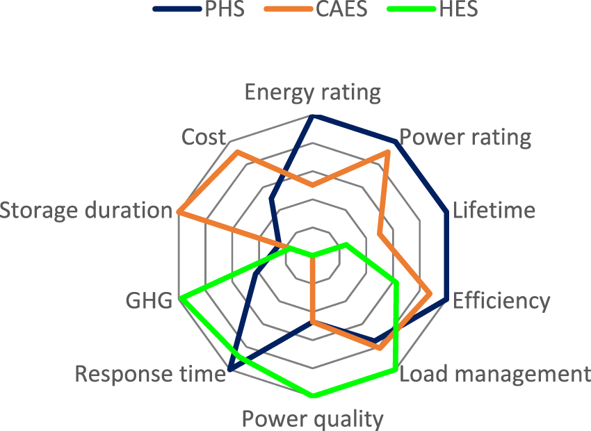
PHS, CAES, and HES are SES options offering storage durations of 6 months, >1 year, and a few months, respectively. There are ten performance indicators for these energy storage systems. These are the energy rating (0.01–10 GWh), power rating (1–1000 MW), lifetime (15–60 years), efficiency (50%–80%), load management (60%–80%), power quality (40%–85%), response time (30 ms to 15 min), GHGs (8–368 g CO2e/kWh), storage duration (months to years), and cost ($400–10000/kW). A comparison between their performance indicators is shown in Figure 5; their dimensionless ratios with respect to the maximum values are scaled to 100 as . For the response time, GHG, and cost, it is more desirable to have lower values. For these three indicators, is applied to scale the values to show consistently higher performing systems at the higher scale. Thus, a system having an outer bound (100) for the indicator is the best, and a system with a lower bound (0) for the indicator is the worst performing system in the radar diagram shown in Figure 5. Thus, PHS has the highest performance in terms of energy and power ratings, lifetime, efficiency, and response time. In terms of storage duration and cost, CAES has the best and HES has the worst performances. HES has the highest load management, power quality, and GHG performances. Load management refers to the extent of load leveling, in which cheap electricity is used during off-peak hours for charging, while discharging takes place during the peak hours to provide cost savings to the operators. Electrical power quality refers to the extent of voltage, frequency, and waveform specifications achieved by a power supply system. Furthermore, PHS and CAES are mature systems, while HES has only started to become available. PHS and CAES have stationary applications, while HES can be used in both stationary and mobile applications.
FIGURE 5
Comparison of the performance indicators between PHS, CAES, and HES.
4 Results of the case study for the energy-intensive southern region of the United Kingdom
The southern part of UK is selected for this case study because it is a demand-intensive temperate region. This region is split into three regions, namely southwest, Greater London, and southeast. The southern region is chosen because it represents UK’s high renewable supply with medium-to-high demand (southwest), low supply with medium demand (Greater London), and high supply with high demand (southeast) scenarios (Sadhukhan et al., 2022). There are fifteen weather stations identified in these three regions, from which hourly wind speed and solar radiation data are compiled (Figure 6). The input data for the optimization model comprises time-series weather data (wind speed and solar radiation) and demand profiles (Figure 1). The hourly-resolution annual wind speed and solar radiation data of the weather stations are obtained from the Centre for Environmental Data Analysis (Available atb; Available atc). The southwest region also has equally sparse hourly weather data and area mean approximations. Some concentrated weather stations collect hourly data around the Greater London region.
FIGURE 6

Locations of the (A) weather stations with (B) hourly wind speed and solar radiation heat maps for the case study.
4.1 Climatology
Hourly weather data from the Centre for Environmental Data Analysis (CEDA) were analyzed for the energy-intensive United Kingdom South region from 2017 onwards with the most complete and consistent datasets. These datasets were fed into the NLP model. The hourly wind and solar generation profiles obtained from the NLP solution (Python-Pyomo IPOPT-GAMS optimizer) were then analyzed along with the demand profiles of benchmark energy storage discharge time by RADA, beyond which the costs and GHGs increase rapidly for the highest electricity-consuming region of United Kingdom South.
The hourly wind speed and solar radiation data were analyzed from fifteen weather stations from 2017 onwards (Available atb; Available atc). The wind and solar power generation models are climate-dependent (wind speed and solar radiation) non-linear models rendering the power system optimization as an NLP problem. The hourly weather data from the various weather stations were complete from 2017. Datasets prior to 2017 have lower spans, high uncertainties, and data gaps at the subnational levels and were thus omitted from the representative average calculations. The data protection policy by CEDA allows statistical representations rather than raw data presentations for educational and research purposes. Thus, the average annual hourly wind speed and solar radiation data analysis results are shown herein. The data source is an ftp server maintained by CEDA. A Visual Studio Code requests CSV files with a regex pattern for this purpose (Available atd). This code recursively downloads the CEDA climate data for the local destination; the time, wind speed, and solar radiation data can thus be accessed through a script for analyzing the climate data. Further, automated data cleaning omits locations for which the data availability is too sparse. Fifteen locations were thus chosen for the South of the United Kingdom, and clean granular wind speed and solar radiation datasets were curated for the most complete data collection years from 2017 onwards.
The study focuses on areas in the South of the United Kingdom, which are split into three regions as southwest, Greater London, and southeast, which had populations of 5.7 million, 9 million, and 9.2 million, respectively, as of 2020. The southeast region had the highest average electricity consumption of 3,984 kWh/m, exceeding the 4,600 kWh/m of Greater London and 3,800 kWh/m of the southwest region (Available ate). The South of the United Kingdom has the highest annual electricity demand at 80 TWh, accounting for 27% of the consumption by the United Kingdom. The southwest, Greater London, and southeast regions consumed 25, 17, and 38 TWh, respectively. Eight weather stations span the southwest region having an area of 31,119 km2 spanning 51.8767° N to 50.2° N latitude and 5.33° W to 1.7247° W longitude. There are four and three weather stations each in the southeast and Greater London regions, which have areas of 23,265 km2 and 4,707 km2, respectively, spanning 1.3703° E to the Eastern coast of the UK.
The hourly wind speeds and solar radiation of the three regions are presented in two ways. The histograms of the wind speeds for each of the four seasons (first quarter: Jan–Mar, second quarter: Apr–Jun, third quarter: Jul–Sep, and fourth quarter: Oct–Dec) for each region are shown in Figure 7 (Available atf). The median, 50th percentile, and 95th percentile daily solar radiation cycles for each of the four seasons for each region are shown in Figure 8 (Available atg). The critical characteristics of the two types of energy systems (wind and solar) are best analyzed with the seasonal variations and seasonal–daily cycles, respectively. Wind speed has seasonal variations, unlike solar radiation, which is only available 50% of the time based on the daily mean.
FIGURE 7

Frequency distributions for wind speeds during the four quarters in the three regions. The red bars indicate the probabilities of the cut-in wind speeds less than 4 m/s.
FIGURE 8

Seasonal daily solar radiation cycles during the four quarters in the three regions. The darker areas show the data coverage within the 50th percentile. The outer lighter areas show the data coverage within the 95th percentile.
The cut-in speed () for wind power generation is 4 m/s. Wind power generation was unavailable (wind speed < 4 m/s) for approximately 185, 775, and 450 h in the first quarter; 350, 1,030, and 300 h in the second quarter; 350, 1,000, and 400 h in the third quarter; and 340, 700, and 200 h in the fourth quarter. Thus, the probability of no wind power generation was the highest for Greater London. The observations were pretty similar between the second and third quarters and between the first and fourth quarters, except for the southwest region, where the observations were identical except for the first quarter. Above 13.5–17, 9–10, and 13–16 m/s wind speeds in the southwest, Greater London, and southeast regions occurred for less than 100 h in each quarter. The cut-out speed () for wind power generation is 25 m/s. The maximum probability (above 4 m/s) occurs for wind speeds of up to 10, 7, and 9 m/s in the three regions. The UK’s prevailing winds are from the southwest region, which manifest with a broad wind speed distribution above the mean value. The extreme West (latitude: 50° 12′ 45.972″ N and longitude: 5° 17′ 41.19″ W) and East (51.3458° N, 1.3703° E) locations have average wind speeds of 10.33 m/s and 7.71 m/s, respectively. The North (51.8767° N, 1.7247° W) also has some of the highest average recorded value of 10 m/s.
October to March show significantly shorter durations of solar radiation and lower radiation intensities. Nearly 50% of the solar radiation received in these months is less than 1,000 kJ/m2 between 8:00 and 16:00 h. The maximum solar radiation is in the second quarter, with values between 1,000 and 2,500 kJ/m2. In the second and third quarters, between 11:00 and 15:00 h, the median solar radiation values are above 1,000 kJ/m2 for the three regions. The solar radiation decreases in order during the second, third, first, and fourth quarters. Solar radiation makes a difference for power generation from 7:00 and 9:00 h during the second–third and first–fourth quarters, respectively. The solar radiation maximum is post-noon and starts diminishing from 23:00 and 20:00 h during the second–third and first–fourth quarters, respectively.
Wind speeds are significant during October–March, while solar radiation is significant over April–September. The median solar radiation is zero for October–March. Thus, wind electricity dominates during October–March, and solar electricity is more significant than wind electricity during April–September. Solar radiation has several thousand manifolds higher variances than wind speed in every way, seasonally and in the three geographic study regions. The variances for wind speed are the least for the Greater London region. The southwest, southeast, and Greater London regions have decreasing wind speeds and solar radiation, in that order. Greater London has the weakest wind speed, with a median value of <6 m/s. Wind speed is higher and fluctuates more in the southwest and southeast regions.
4.2 Demand time-series
The hourly electricity demand profiles (annual hourly resolution) are available for the United Kingdom only at the national level (Available atg). The hourly electricity demands are needed for the hourly electricity and total balance in Eq. (3a, 3b). The subnational annual total electricity demands are publicly available data (Available ate). The yearly mean electricity demands of the regions are calculated based on the weighted area averages of the annual local demands. Then, the electricity demand profiles (hourly resolution) are generated for the regions by downscaling the national electricity demand profiles (hourly resolution) for the calculated annual local mean demands. The data analytics and visualization of the subnational electricity demand profiles are discussed in the following section on electricity (wind plus solar) supply and demand analyses.
5 Results and discussion
The NLP model in Figure 1 and Supplementary Material were created with Visual Studio Code (Available ath) and can be implemented on a standard computer; the solution in terms of the optimal electricity mix is obtained in less than 1 min on a Dell Latitude E5570 device. Figure 9 (Available atf) shows the resulting monthly wind and solar electricity generations along with the superimposed electricity demand and wind plus solar power profiles from the NLP model (Available ath) in the three regions. Combining wind and solar generations is beneficial in many ways. The seasonal variations of wind speed and daily cycles of solar radiation can complement each other to a certain extent. Night-time electricity demands can be met by wind power when there is no solar generation. The low solar generation during the first and fourth quarters can be complemented by wind generation. Their individual and combined generations were analyzed with the electricity load demand in spatiotemporal resolution to characterize the combined energy storage discharge regimes.
FIGURE 9

Monthly wind and solar power generation and superimposed electricity demand and generation based on wind plus solar sources. The darker areas show the data coverage within the 50th percentile. The outer lighter areas show the data coverage within the 95th percentile.
The seasonal variations of wind speed and daily cycles of solar radiation impact wind and solar power generation. Figure 9 includes the 50th and 90th percentile data spreads of electricity usage. Solar power peaks at more than 2,000 MWh between 8:00 and 13:00 h, when 50% of the wind power is less than 5,000 MWh. Unlike wind speed, wind power has higher variance than solar power. The total of wind and solar generation has a higher proportion of wind power than solar power. The median wind power and its variance are lowest for the Greater London region. The median and variance values of electricity demand are also the lowest for the Greater London region. southeast region has the highest electricity demand (38 TWh), which is over 2.2 times that of Greater London (17 TWh) and about 1.6 times that of the southwest region (25 TWh). The highest electricity demand in the southeast region explains why wind plus solar power cannot fulfill the higher electricity demand in this region. The combined wind and solar power may be excess from March to September in the southwest and Greater London regions. In the case of the southeast region, the combined wind and solar generation data spread mostly falls under the demand profile; this suggests that lower amounts of wind and solar power generated can directly reduce demand without energy storage. The demand dataset has a narrower distribution than the combined wind and solar generation datasets.
Figure 10 shows the daily median electricity demand and wind plus solar electricity generation profiles over the four quarters in the three regions. The Greater London region accounts for lower demand and lower supply than the two other regions. Between 8:00 and 16:00 h over Oct–Mar, the demand (less than 4,000 MWh) is less than supply for the Greater London and southwest regions, while the southeast region has a demand exceeding 4,000 MWh. The combined wind and solar power cannot fully meet the electricity demands over Oct–Mar. The surplus energy available for storage is insignificant, and the energy storage duration required to meet the demand is significant. Demand is greater than supply every day in each quarter, except between April and September (second and fourth quarters). The demand peaks between 17:00 and 19:00 h and is steadily high at other times after 7:00 h for all quarters in the three regions. The gap between demand and wind plus solar electricity supply (i.e., deficit) is highest around 19:00 h; this is the time when the after-work domestic electricity usage is maximum. The electricity demand is higher in Oct–Mar than Apr–Sep because the lights are on longer and some houses use electricity for heating due to the low solar radiation. The only time when the combined wind and solar supply is greater than demand is during mid-day and afternoon in the second and third quarters, when energy storage is needed to store the excess energy in the case of the southwest and Greater London regions. For the southeast region, the combined wind and solar supply is still insufficient to meet the electricity load in Apr–Sep, and power may be dispatched to reduce the demand directly without energy storage. In Apr–Sep, the solar power contribution is dominant; the availability of solar power makes a difference in the electricity output between 9:00 and 15:00 h. This excess electricity can support the transportation sector that primarily uses fossil-based fuels in the absence of adequate SES.
FIGURE 10

Daily median electricity demands as well as combined wind and solar electricity generation profiles over the four quarters in the three regions. The darker areas show the data coverage within the 50th percentile. The outer lighter areas show the data coverage within the 95th percentile.
The load demands have median values (in MW) of 3,043, 2,453, 2,399, and 2,930 (southwest); 2,218, 1,788, 1,749, and 2,136 (Greater London); and 4,864, 3,922, 3,835, and 4,684 (southeast) for the Jan–Mar, Apr–Jun, Jul–Sep, and Oct–Dec quarters, respectively. Their variances (summation of the squared variations between the individual sample points and their mean, divided by one less than the number of sample points) are 332,234, 142,236, 151,027, and 386,686 (southwest); 183,314, 75,560, 80,229, and 205,418 (Greater London); and 881,677, 363,416, 385,875, and 987,987 (southeast) for the Jan–Mar, Apr–Jun, Jul–Sep, and Oct–Dec quarters, respectively, as detailed in Sadhukhan et al. (2022).
5.1 Energy storage dispatch durations from surplus and deficit power profile analyses
Figure 11 (top) shows the surplus and deficit electricity values after balancing the combined wind and solar generations with the electricity load demand every hour for each region. These profiles show the non-coincident surplus and deficit power without energy storage. The deficit electricity is shown as a negative profile to differentiate it from the surplus. Other renewable and carbon-efficient technologies can meet the electricity deficit. Surplus electricity can displace other forms of energy, such as transport fuels providing electrification for the transportation sector. It is noted that the agricultural (Martinez-Hernandez et al., 2013; Martinez-Hernandez et al., 2014; Martinez-Hernandez et al., 2022), aviation (Sadhukhan et al., 2014; Sadhukhan and Sen, 2021), and heavy industry (Sadhukhan et al., 2004; Sadhukhan et al., 2017; Shemfe et al., 2018) sectors (whole lifecycle systems) are the toughest to electrify owing to their high-quality heating/fuel requirements. However, energy storage is inevitable for the excess wind and solar power generated because of interseasonal and interannual variabilities. Figure 11 (bottom) shows the surplus and deficit electricity profiles after the feasible stored energy transfer reduces demand for each region.
FIGURE 11

For each region, the annual electricity surplus and deficit profiles are shown after balancing supply and demand every hour without energy storage (top) along with the electricity surplus and deficit profiles with energy storage (bottom).
The surplus electricity over a given hour is zero if it is less than the demand over that hour; this means that the available wind and solar power are completely dispatched at the given time and that the demand may still not be met. Otherwise, the surplus electricity is the difference between the supply and demand (supply > demand). The deficit electricity over a given hour is zero if it is less than the supply over the same hour; otherwise, the deficit electricity is the difference between the demand and supply (demand > supply). These operations are performed by generating the energy storage duration () randomly within any given storage duration, 0 < < , for each time resolution step () until all time resolution steps are exhausted (by applying the RADA calculations shown in Figure 3).
After deploying the stored energy, the second and third quarters have surplus wind and solar electricity, whereas the first and fourth quarters have a deficit of wind and solar electricity. Solar radiation primarily impacts the shapes and sizes of these profiles. Remarkably, because of the highest electricity demand in the southeast region, all surplus wind and solar electricity can be utilized to reduce the demand deficit after applying energy storage, and there will still be unmet load demand, for which other forms of dispatchable power supply must be sought.
Figure 12 shows the relationship for reliability (percentage of electricity demand met by excess wind and solar or other renewable power in each discharge time or the ratio between combined wind and solar non-coincided power discharge and total demand) against the stored energy discharge time. These profiles have some common characteristics as follows: the highest slope within the first 4 h of stored energy dispatch time, a lower slope over 4–87 h of discharge time, and almost no improvement in the percentage reliability above 96 h of stored energy discharge time. Based on the fractional values of reliability, these slopes are 0.014–0.025 h-1, 0.0008–0.0014 h-1, and 0.00009–0.0002 h-1 for <4 h, 4–87 h, and 87–168 h of energy storage, respectively. Beyond 168 h of energy storage, the reliability shows only an infinitesimal increment. BESSs offer such energy storage durations (Sadhukhan and Christensen, 2021).
FIGURE 12

Percentage reliability against stored energy discharge time.
5.2 Seasonal storage evaluation mapping for integration with wind and solar generation and comparison against bioenergy and gas with CCS
About 63%, 62%, and 55% of the annual electricity demands (25, 17, and 38 TWh annually) can be met directly with dispatchable wind and solar power without energy storage in the southwest, Greater London, and southeast regions, respectively. Further, stored energy can provide 21%, 22%, and 13% of the current electricity demands after 4 days of storage (13.5 TWh out of the total demand of 80 TWh annually in the South of the United Kingdom). The greater the demand, the less is the electricity demand met by energy storage. Thus, wind and solar power can meet 15.8 TWh, 10.5 TWh, and 20.9 TWh of energy demands in the southwest, Greater London, and southeast regions, respectively, without energy storage. Further, BESSs can store 5.3 TWh, 3.7 TWh, and 4.9 TWh of wind and solar energy up to a feasible storage duration of 1 week in these three regions, as shown in Section 4.1. The unmet demands in the three regions would then be 4 TWh, 2.7 TWh, and 12.2 TWh. Figure 13 illustrates the annual electricity demands met by direct wind and solar power, wind and solar with battery energy storage, and the unmet demand.
FIGURE 13

Directly dispatchable wind and solar energy, battery energy storage, and unmet electricity demand distributions in the three regions of the United Kingdom South.
The remaining electricity demands can be met by non-coincident wind and solar power through the incorporation of SES systems like PHS, CAES, and HES. The unmet demands can be met by these SES systems or directly by dispatchable power from bioenergy and gas with CCS systems (nuclear energy is not considered here because of its waste disposal cost implications). Thus, all these options need to be compared for costs (using Eq. (4)) and GHGs (based on Figure 4), as shown in Figure 14.
FIGURE 14

(top) Costs, (middle) GHG, and (bottom) cost per unit GHG to meet the 4 TWh, 2.7 TWh, and 12.2 TWh of electricity demands in the three regions through various options: PHS, CAES, HES, gas with CCS, bioenergy, and wind and solar integrated with PHS, CAES, and HES.
The suitable systems based on increasing order of costs are CAES < gas with CCS < PHS < bioenergy < HES (Figure 14 (top)). The solar or wind power (at $36/MWh and $108/MWh in Figure 4) integrated CAES is still the minimal cost choice. The systems based on increasing order of GHGs are HES < bioenergy < gas with CCS < CAES < PHS (Figure 14 (middle)). The systems based on increasing order of cost per GHG (EURO/kg CO2e) are solar + CAES < wind + CAES < solar + PHS < wind + PHS < gas with CCS < bioenergy < solar + HES < wind + HES (Figure 14 (bottom)). As the minimum cost choice, CAES also has the least cost per GHG when integrated with solar and wind electricity. Gas with CCS is a better option than bioenergy and HES with solar or wind electricity based on the cost per GHG. The UK’s NZE by 2035 can thus be met predominantly by renewable self-generation, first through coincided renewable power and then by non-coincided solar and wind power through battery energy storage, followed by non-coincided solar and wind power through SES options like CAES and PHS. Dispatchable wind and solar energy can meet 63%, 62%, and 55% (15.8, 10.5, and 20.9 TWh) of the electricity demands in the southwest, Greater London, and southeast regions, respectively. Further, BESSs can increase the wind and solar energy in the NZE mix in the three regions by 5.3, 3.7, and 4.9 TWh. The proportions of wind and solar electricity availabilities are 65:35, 62:38, and 66:34 in these three regions. The remaining demand of 4, 2.7, and 12.2 TWh can be met by solar + CAES < wind + CAES < solar + PHS < wind + PHS < gas with CCS < bioenergy < solar + HES < wind + HES based on increasing order of cost per GHG of 0.33, 0.69, 0.84, 1.13, 2.18, 5.89, 8.54, and 26.97 EURO/kg CO2e, respectively. However, owing to the infinitesimal increment in reliability beyond 96 h of energy storage provided by BESSs, gas with CCS or bioenergy is likely to meet the balance load demand (4, 2.7, and 12.2 TWh).
A value analysis diagram (Sadhukhan et al., 2003; Sadhukhan et al., 2004; Sadhukhan et al., 2008; Sadhukhan et al., 2014) is shown in Figure 15, which is a plot of the levelized cost of electricity in EURO/MWh along the y axis versus annual electrical energy supply in TWh along the x axis. Figure 15 shows the electrical energy contributions from direct solar and wind, indirect solar and wind with BESS, and indirect solar and wind with CAES systems at various levelized costs of electricity. For example, direct solar electrical energy supply is 16.5 TWh at the levelized cost of electricity of 32.4 EURO/MWh. The area bounded by the direct solar energy (parallel line to the x axis) and x axis is the total cost incurred by the direct solar electrical energy supply, i.e., million EURO. Direct wind provides or 30.7 TWh of electrical energy at the levelized cost of electricity of 97.2 EURO/MWh. Next, solar and wind electrical energy supply with BESS accounts for or 4.9 TWh and or 9 TWh at the levelized costs of electricity of 41.1 and 105.9 EURO/MWh, respectively. Thereafter, the least-cost solar and wind electrical energy supply with CAES from among all the SES options accounts for or 6.5 TWh and or 12.4 TWh at the levelized costs of electricity of 95.2 and 160 EURO/MWh, respectively. Thus, the total solar and wind electrical energy contributions from direct, indirect BESS, and indirect CAES systems are 47.2 TWh, 13.9 TWh, and 8.9 TWh at the levelized costs of electricity of 75, 83, and 138 EURO/MWh, respectively. The resulting overall levelized cost of electricity is 91 EURO/MWh, which is less than the previously obtained levelized cost of electricity (Sadhukhan et al., 2022). The cost contributions (million EURO/year) are as follows: direct solar: 536, direct wind: 2,981, indirect solar with BESS: 201, indirect wind with BESS: 953, indirect solar with CAES: 622, and indirect wind with CAES: 1978; these account for costs of 3,517, 1,154, and 2,600 for the direct, indirect with BESS, and indirect with CAES options, respectively. Thus, an overall cost of 7.3 billion EURO/year will be incurred to achieve NZE for the South of UK.
FIGURE 15

Levelized cost of electricity (EURO/MWh) versus annual electrical energy contributions (TWh) for the individual components (green), total direct, indirect with BESS, indirect with CAES (red), and overall (grey) cases.
Because of the infinitesimal increment in reliability beyond 96 h of energy storage needing SES, gas with CCS or bioenergy could be likely candidates for meeting the balance load demands (4, 2.7, and 12.2 TWh in the three regions). Gas with CCS and bioenergy can increase the overall levelized cost of electricity by 112 and 145 EURO/MWh, i.e., 9–11 billion EURO/year in costs, which is an increase from 7.3 billion EURO/year for CAES to meet the balance load demands for NZE for UK South.
Our NLP optimization model suggests the following optimal electricity mix: 55% wind, 29% solar, 0.5% hydro, 0.4% geothermal, and 1% bioenergy (high supply with medium-to-high demand); 52% wind, 32% solar, 0.5% hydro, 0.5% geothermal, and 1% bioenergy (low supply with medium demand); 45% wind, 23% solar, 0.7% hydro, 0.7% geothermal, and 10% bioenergy (high supply with high demand) (Sadhukhan et al., 2022). The resulting least levelized cost of electricity was 120 EURO/MWh (Sadhukhan et al., 2022). The NZE projections for the whole of United Kingdom would be wind: 40 GW, solar: 21 GW, bioenergy and other renewables: 5 GW, nuclear: 6 GW, and gas with CCS: 5 GW by 2050, which mirrors the government’s NZE plan for the entire United Kingdom, with 670 TWh or 77 GW in the high-innovation scenario (Sadhukhan et al., 2022). With the CAES integration proposed in this work, there is an expected annual savings of 19.5 billion EURO (i.e., 29 EURO/MWh) by displacing gas with CCS, bioenergy, and nuclear sources in the previous study for the NZE of the whole of United Kingdom (670 TWh or 77 GW in the high-innovation scenario (Sadhukhan et al., 2022)).
The cost and Ecoinvent-based GHG parameters for the energy storage systems are derived from reliable as well as universally accepted and respected sources (Bogdanov et al., 2019; Bogdanov et al., 2021; Sadhukhan, 2021). Their temporal variations could still occur, especially with the learning curve effects (Sadhukhan et al., 2004). However, decisions made by models are less sensitive to the absolute values of these parameters than relative values, which are unlikely to change. Hence, the conclusions are less likely to change, as seen in other studies (Lund and Vad Mathiesen, 2009; Bogdanov et al., 2019; Bogdanov et al., 2021). The spatial variations of the cost parameters are less likely as the market is global. This work employs the NLP approach for optimization of the NZE system. This approach is comprehensive, as it accounts for various costs (capital, fixed, variable, resource, pollution, upgrading, and decommissioning), capacity-factor-based wind and solar power generations, and levelized parameters. The comprehensive model with the right level of complexity remains practical and interpretable. The methodological framework presented herein is generic and may be extended to include further energy storage options and other geographic regions.
6 Conclusion
A novel framework integrating NLP, RADA, and SES performance evaluations is used herein to maximize the technoeconomic and environmentally feasible NZE mix. Spatiotemporal climate/geophysical/meteorological and electrical load demand data are used to constrain the optimization problem. The total cost objective, including the weighted average capital, fixed, variable, resource, pollution (including GHG), upgrading, and decommissioning costs, over a designated time scale (e.g., annual, decadal, or multidecadal) is formulated, and the spatiotemporal variations of the energy storage systems are captured using non-linear regression equations. The constraints include upper and lower bounds of each unit capacity in the entire energy system and energy balance equations at the finest time resolution. Adherence to the energy balance principles is ensured while accounting for power generation, storage, losses, and load requirements.
The UK’s NZE by 2035 can thus be met predominantly by renewable self-generation, first by coincided renewable power and then by non-coincided solar and wind power through battery energy storage, followed by non-coincided solar and wind power through SES like CAES and PHS. Dispatchable wind and solar energy can meet 63%, 62%, and 55% (15.8, 10.5, and 20.9 TWh) of the electricity demands in the southwest, Greater London, and southeast regions, respectively. Further, BESSs increased the wind and solar energy portions in the NZE mix by 5.3, 3.7, and 4.9 TWh for the above three regions. Correspondingly, the proportions of wind and solar electricity availabilities are 65:35, 62:38, and 66:34 in these three regions. The balance demands (4, 2.7, and 12.2 TWh) can be met by solar + CAES < wind + CAES < solar + PHS < wind + PHS < gas with CCS < bioenergy < solar + HES < wind + HES based on increasing order of cost per GHG as 0.33, 0.69, 0.84, 1.13, 2.18, 5.89, 8.54, and 26.97 EURO/kg CO2e, respectively. However, given the infinitesimal increment in reliability beyond the 96 h of energy storage provided by BESS, gas with CCS or bioenergy can likely meet the balance load demands (4, 2.7, and 12.2 TWh). Policymakers, investors, and power system operators are thus provided with actionable insights to facilitate informed decision-making regarding energy infrastructure investments and policy formulation.
Statements
Data availability statement
The datasets presented in this study can be found in online repositories. The names of the repositories and accession numbers can be found below: https://github.com/sohumsen/power_systems_optimization.
Author contributions
JS: Conceptualization, Data curation, Formal analysis, Funding acquisition, Investigation, Methodology, Project administration, Resources, Software, Supervision, Validation, Visualization, Writing–original draft, Writing–review and editing. SS: Data curation, Formal analysis, Software, Validation, Visualization, Writing–review and editing. TR: Software, Visualization, Writing–review and editing.
Funding
The authors declare that financial support was received for the research, authorship, and/or publication of this article. The authors acknowledge research support from the University of Surrey.
Acknowledgments
The UKRI (BB/Y008456/1, EP/Y005600/1, BB/X011372/1, BB/X011615/1, BB/S009795/1 and TS/X017648/1) has been acknowledged to support this research.
Conflict of interest
The authors declare that the research was conducted in the absence of any commercial or financial relationships that could be construed as a potential conflict of interest.
Publisher’s note
All claims expressed in this article are solely those of the authors and do not necessarily represent those of their affiliated organizations or those of the publisher, editors, and reviewers. Any product that may be evaluated in this article or claim that may be made by its manufacturer is not guaranteed or endorsed by the publisher.
Supplementary material
The Supplementary Material for this article can be found online at: https://www.frontiersin.org/articles/10.3389/fenrg.2024.1430413/full#supplementary-material
References
1
Aboumahboub T. Schaber K. Tzscheutschler P. Hamacher T. (2010). Optimization of the utilization of renewable energy sources in the electricity sector. Renew. Energy Resour.11, 13–14.
2
Al-Ghussain L. Ahmed H. Haneef F. (2018). Optimization of hybrid PV-wind system: Case study Al-Tafilah cement factory, Jordan. Sustain Energy Technol. Assess.30, 24–36. 10.1016/j.seta.2018.08.008
3
Alirahmi S. M. Razmi A. R. Arabkoohsar A. (2021). Comprehensive Assessment and Multi-Objective Optimization of A Green Concept Based on a Combination of Hydrogen and Compressed Air Energy Storage (CAES) Systems. Renew. Sustain. Energy Rev.142, 110850. 10.1016/j.rser.2021.110850
4
AlShafi M. Bicer Y. (2021). Life Cycle Assessment of compressed air, Vanadium Redox Flow Battery, and Molten Salt Systems for Renewable Energy Storage. Energy Rep.7, 7090–7105. 10.1016/j.egyr.2021.09.161
5
Anoune K. Laknizi A. Bouya M. Astito A. Abdellah A. B. (2018). Sizing a PV-Wind Based Hybrid System Using Deterministic Approach. Energy Conv. Manage169, 137–148. 10.1016/j.enconman.2018.05.034
6
Argyrou M. C. Christodoulides P. Kalogirou S. A. (2018). Energy Storage for Electricity Generation and Related Processes: Technologies Appraisal and Grid Scale Applications. Renew. Sustain Energy Rev.94, 804–821. 10.1016/j.rser.2018.06.044
7
Atzeni I. Ordóñez L. G. Scutari G. Palomar D. P. Fonollosa J. R. (2012). Demand-Side Management Via Distributed Energy Generation and Storage Optimization. IEEE Trans. Smart Grid4, 866–876. 10.1109/TSG.2012.2206060
8
Augutis J. Martišauskas L. Krikštolaitis R. (2015). Energy mix optimization from an energy security perspective. Energy Conv. Manag.90, 300–314. 10.1016/j.enconman.2014.11.033
9
Available at: https://www.nrel.gov/docs/fy04osti/35404.pdf.
10
11
12
Available at: ftp.ceda.ac.uk.
13
14
Available at: https://github.com/tsinampoizina/wind_solar_energy.
15
Available at: https://www.gridwatch.templar.co.uk/download.php.
16
Available at: https://github.com/sohumsen/power_systems_optimization.
17
Bakhtvar M. Al H. A. El Moursi M. S. Albadi M. H. (2021). A Vision of Flexible Dispatchable Hybrid Solar-Wind-Energy Storage Power Plant. IET Renew. Power Gener.15, 2983–2996. 10.1049/rpg2.12234
18
Bogdanov D. Farfan J. Sadovskaia K. Aghahosseini A. Child M. Gulagi A. et al (2019). Radical Transformation Pathway Towards Sustainable Electricity Via Evolutionary Steps. Nat. Commun.10, 1077–1116. 10.1038/s41467-019-08855-1
19
Bogdanov D. Ram M. Aghahosseini A. Gulagi A. Oyewo A. S. Child M. et al (2021). Low-cost Renewable Electricity as the Key Driver of the Global Energy Transition Towards Sustainability. Energy227, 120467. 10.1016/j.energy.2021.120467
20
Brouwer A. S. van den Broek M. Zappa W. Turkenburg W. C. Faaij A. (2016). Least-Cost Options for Integrating Intermittent Renewables in low-Carbon Power Systems. Appl. Energy161, 48–74. 10.1016/j.apenergy.2015.09.090
21
Brown T. Schlachtberger D. Kies A. Schramm S. Greiner M. (2018). Synergies of Sector Coupling and Transmission Reinforcement in a Cost-Optimised, Highly Renewable European Energy System. Energy160, 720–739. 10.1016/j.energy.2018.06.222
22
Denholm P. Margolis R. M. (2007). Evaluating the Limits of Solar Photovoltaics (PV) in electric Power Systems Utilizing Energy Storage and Other Enabling Technologies. Energy Policy35 (9), 4424–4433. 10.1016/j.enpol.2007.03.004
23
Dorfner J. (2016). Open source modelling and optimisation of energy infrastructure at urban scale. Technische Universität München. Doctoral dissertation.
24
Dowling J. A. Rinaldi K. Z. Ruggles T. H. Davis S. J. Yuan M. Tong F. et al (2020). Role of long-duration energy storage in variable renewable electricity systems. Joule4 (9), 1907–1928. 10.1016/j.joule.2020.07.007
25
Firatoglu Z. A. Yesilata B. (2004). New approaches on the Optimization of Directly Coupled PV Pumping Systems. Sol. Energy77, 81–93. 10.1016/j.solener.2004.02.006
26
Franco A. Salza P. (2011). Strategies for Optimal penetration of Intermittent Renewables in Complex Energy Systems Based on Techno-Operational Objectives. Renew. Energy36, 743–753. 10.1016/j.renene.2010.07.022
27
Gil G. O. Chowdhury J. I. Balta-Ozkan N. Hu Y. Varga L. Hart P. (2021). Optimising renewable energy integration in new housing developments with low carbon technologies. Renew. Energy169, 527–540. 10.1016/j.renene.2021.01.059
28
Houssainy S. Livingood W. (2021). Optimal Strategies for a Cost-Effective and Reliable 100% Renewable Electric Grid. J. Renew. Sustain Energy13, 066301. 10.1063/5.0064570
29
Jane R. Parker G. Vaucher G. Berman M. (2020). Characterizing Meteorological Forecast Impact on Microgrid Optimization Performance and Design. Energies13, 577. 10.3390/en13030577
30
Khalid M. Ahmadi A. Savkin A. V. Agelidis V. G. (2016). Minimizing the Energy Cost For Microgrids Integrated With Renewable Energy Resources And Conventional Generation Using Controlled Battery Energy Storage. Renew. Energy97, 646–655. 10.1016/j.renene.2016.05.042
31
Li Z. Zhi X. Wu Z. Qian G. Jiang R. Wang B. et al (2023). Role of different energy storage methods in decarbonizing urban distributed energy systems: A case study of thermal and electricity storage. J. Energy Storage73, 108931. 10.1016/j.est.2023.108931
32
Lu B. Blakers A. Stocks M. Do T. N. (2021). Low-cost, Low-Emission 100% Renewable Electricity in Southeast Asia Supported by Pumped Hydro Storage. Energy236, 121387. 10.1016/j.energy.2021.121387
33
Lund H. Vad Mathiesen B. (2009). Energy System Analysis of 100% Renewable Energy Systems—The Case of Denmark in Years 2030 and 2050. Energy34, 524–531. 10.1016/j.energy.2008.04.003
34
Martinez-Hernandez E. Ibrahim M. H. Leach M. Sinclair P. Campbell G. M. Sadhukhan J. (2013). Environmental Sustainability Analysis of UK Whole-Wheat Bioethanol and CHP Systems. Biomass Bioenergy50, 52–64. 10.1016/j.biombioe.2013.01.001
35
Martinez-Hernandez E. Martinez-Herrera J. Campbell G. M. Sadhukhan J. (2014). Process Integration, Energy and GHG Emission Analyses of Jatropha-Based Biorefinery Systems. Biomass Conv. Bioref4, 105–124. 10.1007/s13399-013-0105-3
36
Martinez-Hernandez E. Sadhukhan J. Aburto J. Amezcua-Allieri M. A. Morse S. Murphy R. (2022). Modelling to Analyse the Process and Sustainability Performance of Forestry-Based Bioenergy Systems. Clean. Tech. Environ. policy24, 1709–1725. 10.1007/s10098-022-02278-1
37
Mazzeo D. Herdem M. S. Matera N. Bonini M. Wen J. Z. Nathwani J. et al (2021b). Artificial intelligence application for the performance prediction of a clean energy community. Energy232, 120999. 10.1016/j.energy.2021.120999
38
Mazzeo D. Matera N. De Luca P. Baglivo C. Congedo P. M. Oliveti G. (2021a). A literature Review And Statistical Analysis Of Photovoltaic-Wind Hybrid Renewable System Research by Considering The Most Relevant 550 Articles: An Upgradable Matrix Literature Database. J. Clean. Prod.295, 126070. 10.1016/j.jclepro.2021.126070
39
Mazzeo D. Matera N. Oliveti G. (2018). Interaction between a Wind-PV-Battery-Heat Pump Trigeneration System and Office Building Electric Energy Demand Including Vehicle Charging. IEEE Int Conf Environ Electr. Eng IEEE Ind Commer. Power Syst. Eur. (EEEIC/I&CPS Europe), 1–5. 10.1109/EEEIC.2018.8493710
40
Monforti F. Huld T. Bódis K. Vitali L. D'isidoro M. Lacal-Arántegui R. (2014). Assessing complementarity of wind and solar resources for energy production in Italy. A Monte Carlo approach. Renew. Energy63, 576–586. 10.1016/j.renene.2013.10.028
41
Niaei H. Masoumi A. Jafari A. R. Marzband M. Hosseini S. H. Mahmoudi A. (2022). Smart Peer-To-Peer And Transactive Energy Sharing Architecture Considering Incentive-Based Demand Response Programming Under Joint Uncertainty and Line Outage Contingency. J. Clean. Prod.363, 132403. 10.1016/j.jclepro.2022.132403
42
Nikolakakis T. Fthenakis V. (2011). The Optimum Mix of Electricity From Wind-And Solar-Sources in Conventional Power Systems: Evaluating The Case For New York State. Energy Policy39, 6972–6980. 10.1016/j.enpol.2011.05.052
43
Nirbheram J. S. Mahesh A. Bhimaraju A. (2023). Techno-Economic Analysis of grid-Connected Hybrid Renewable Energy System Adapting Hybrid Demand Response Program and Novel Energy Management Strategy. Renew. Energy2023, 1–16. 10.1016/j.renene.2023.05.017
44
Perez-Arriaga I. J. Batlle C. (2012). Impacts of Intermittent Renewables on Electricity Generation System Operation. Econom. Energy Environ. Policy1, 3–18. 10.5547/2160-5890.1.2.1
45
Prebeg P. Gasparovic G. Krajacic G. Duic N. (2016). Long-term Energy Planning of Croatian Power System Using Multi-Objective Optimization With Focus on Renewable Energy and Integration Of Electric Vehicles. Appl. Energy184, 1493–1507. 10.1016/j.apenergy.2016.03.086
46
Rahbari H. R. Arabkoohsar A. Nielsen M. P. Mathiesen B. V. Lund H. (2021). Quantification of Realistic Performance Expectations from Trigeneration CAES-ORC Energy Storage system in Real Operating Conditions. Energy Conv. Manag.249, 114828. 10.1016/j.enconman.2021.114828
47
Razmi A. R. Janbaz M. (2020). Exergoeconomic Assessment with Reliability Consideration of A Green Cogeneration System Based on Compressed Air Energy Storage (CAES). Energy Convers. Manag.204, 112320. 10.1016/j.enconman.2019.112320
48
Sadeghi D. Ahmadi S. E. Amiri N. Marzband M. Abusorrah A. Rawa M. et al (2022). Designing, Optimizing and Comparing Distributed Generation Technologies as A Substitute System for Reducing Life Cycle Costs, CO2 Emissions, And Power Losses In Residential Buildings. Energy253, 123947. 10.1016/j.energy.2022.123947
49
Sadhukhan J. (2021). Net Zero Electricity Systems in Global Economies by Life Cycle Assessment (LCA) considering Ecosystem, Health, Monetization, and Soil CO2 Sequestration Impacts. Renew. Energy184, 960–974. 10.1016/j.renene.2021.12.024
50
Sadhukhan J. (2022). Net-Zero Action Recommendations for Scope 3 Emission Mitigation Using Life Cycle Assessment. Energies15 (15), 5522. 10.3390/en15155522
51
Sadhukhan J. Christensen M. (2021). An in-Depth Life cycle assessment (LCA) of Lithium-ion Battery for Climate Impact Mitigation Strategies. Energies14, 5555. 10.3390/en14175555
52
Sadhukhan J. Joshi N. Shemfe M. Lloyd J. R. (2017). Life Cycle Assessment of Sustainable Raw Material Acquisition for Functional Magnetite Bionanoparticle Production. J. Environ. Manag.199, 116–125. 10.1016/j.jenvman.2017.05.048
53
Sadhukhan J. Mustafa M. A. Misailidis N. Mateos-Salvador F. Du C. Campbell G. M. (2008). Value Analysis Tool for feasibility studies of Biorefineries Integrated with value added production. Chem. Eng. Sci.63 (2), 503–519. 10.1016/j.ces.2007.09.039
54
Sadhukhan J. Ng K. S. Martinez-Hernandez E. (2014). “Biorefineries and Chemical Processes: Design,” in Integration and Sustainability Analysis. Wiley. 10.1002/9781118698129
55
Sadhukhan J. Sen S. (2021). A novel mathematical Modelling Platform for Evaluation of a Novel Biorefinery Design With Green Hydrogen Recovery to Produce Renewable Aviation Fuel. Chem. Eng. Res. Des.175, 358–379. 10.1016/j.cherd.2021.09.014
56
Sadhukhan J. Sen S. Gadkari S. (2021). The Mathematics of life cycle sustainability assessment. J. Clean. Prod.309, 127457. 10.1016/j.jclepro.2021.127457
57
Sadhukhan J. Sen S. Randriamahefasoa T. M. S. Gadkari S. (2022). Energy System Optimization for Net-Zero Electricity. Digit. Chem. Eng.3, 100026. 10.1016/j.dche.2022.100026
58
Sadhukhan J. Zhang N. Zhu X. X. (2003). Value analysis of complex systems and industrial application to refineries. Ind. Eng. Chem. Res.42 (21), 5165–5181. 10.1021/ie020968z
59
Sadhukhan J. Zhang N. Zhu X. X. (2004). Analytical optimisation of industrial systems and applications to refineries, petrochemicals. Chem. Eng. Sci.59, 4169–4192. 10.1016/j.ces.2004.06.014
60
Safaei H. Keith D. W. (2015). How Much Bulk Energy Storage is Needed to Decarbonize Electricity?Energy Environ. Sci.8, 3409–3417. 10.1039/c5ee01452b
61
Sameti M. Haghighat F. (2018). Integration of Distributed Energy Storage Into Net-Zero Energy District Systems: Optimum Design and Operation. Energy153, 575–591. 10.1016/j.energy.2018.04.064
62
Shaner M. R. Davis S. J. Lewis N. S. Caldeira K. (2018). Geophysical Constraints on the Reliability of Solar and Wind Power in the United States. Energy Environ. Sci.11, 914–925. 10.1039/c7ee03029k
63
Shemfe M. B. Gadkari S. Sadhukhan J. (2018). Social Hotspot Analysis and Trade Policy Implications of the use of Bioelectrochemical Systems for Resource recovery from Wastewater. Sustainability10, 3193. 10.3390/su10093193
64
Tan W. N. Gan M. T. Tan Z. L. (2016). Optimization models for demand-side and supply-side scheduling in smart grids. IEEE 16th Int. Conf. Environ. Electr. Eng., 1–5. 10.1109/EEEIC.2016.7555476
65
Terlouw T. AlSkaif T. Bauer C. Van Sark W. (2019). Multi-Objective Optimization of Energy Arbitrage In Community Energy Storage Systems Using Different Battery Technologies. Appl. Energy239, 356–372. 10.1016/j.apenergy.2019.01.227
66
Thangavelu S. R. Khambadkone A. M. Karimi I. A. (2015). Long-term Optimal Energy Mix Planning Towards High Energy Security and Low GHG emission. Appl. Energy154, 959–969. 10.1016/j.apenergy.2015.05.087
67
Tong D. Farnham D. J. Duan L. Zhang Q. Lewis N. S. Caldeira K. et al (2021). Geophysical Constraints on the Reliability of solar and Wind Power Worldwide. Nat. Commun.12, 6146–6212. 10.1038/s41467-021-26355-z
68
Ullah K. Hafeez G. Khan I. Jan S. Javaid N. (2021). A multi-Objective Energy Optimization in Smart Grid With High Penetration Of Renewable Energy Sources. Appl. Energy299, 117104. 10.1016/j.apenergy.2021.117104
69
Watson J. D. Watson N. R. Lestas I. (2017). Optimized dispatch of Energy Storage Systems in Unbalanced Distribution Networks. IEEE Trans. Sustain Energy9, 639–650. 10.1109/TSTE.2017.2752964
70
Weber C. Shah N. (2011). Optimisation based design of a district Energy System for an Eco-town in the United Kingdom. Energy36, 1292–1308. 10.1016/j.energy.2010.11.014
71
Weijermars R. Taylor P. Bahn O. Das S. R. Wei Y. M. (2012). Review of Models And Actors In Energy Mix Optimization–Can Leader Visions and Decisions Align With Optimum Model Strategies for Our Future Energy Systems?Energy Strategy Rev.1, 5–18. 10.1016/j.esr.2011.10.001
72
Wierzbowski M. Lyzwa W. Musial I. (2016). MILP Model for Long-term Energy Mix Planning With Consideration of Power system Reserves. Appl. Energy169, 93–111. 10.1016/j.apenergy.2016.02.003
73
Yao D. L. Choi S. S. Tseng K. J. Lie T. T. (2011). Determination of Short-Term Power Dispatch Schedule For a Wind Farm Incorporated With Dual-Battery Energy Storage Scheme. IEEE Trans. Sustain Energy3, 74–84. 10.1109/TSTE.2011.2163092
74
Yousif M. Ai Q. Wattoo W. A. Jiang Z. Hao R. Gao Y. (2019). Least cost combinations of solar power, wind power, and energy storage system for powering large-scale grid. J. Power Sources412, 710–716. 10.1016/j.jpowsour.2018.11.084
75
Zappa W. van den Broek M. (2018). Analysing the Potential of Integrating Wind and Solar Power in Europe Using Spatial Optimisation Under Various Scenarios. Renew. Sustain Energy Rev.94, 1192–1216. 10.1016/j.rser.2018.05.071
76
Zeyringer M. Price J. Fais B. Li P. H. Sharp E. (2018). Designing Low-Carbon Power Systems for Great Britain in 2050 that are robust to the Spatiotemporal and Inter-Annual Variability of Weather. Nat. Energy3, 395–403. 10.1038/s41560-018-0128-x
77
Zhang X. (2014). A Statistical Approach for Sub-Hourly Solar Radiation Reconstruction. Renew. Energy71, 307–314. 10.1016/j.renene.2014.05.038
78
Zhou S. Wang Y. Zhou Y. Clarke L. E. Edmonds J. A. (2018). Roles of Wind and Solar Energy in China’s Power Sector: Implications of Intermittency Constraints. Appl. Energy213, 22–30. 10.1016/j.apenergy.2018.01.025
Summary
Keywords
energy system optimization, energy planning, battery, pumped hydro storage, compressed air energy storage, hydrogen energy storage
Citation
Sadhukhan J, Sen S and Randriamahefasoa TMS (2024) Framework for optimal energy storage duration for maximum-reliability renewable electricity. Front. Energy Res. 12:1430413. doi: 10.3389/fenrg.2024.1430413
Received
09 May 2024
Accepted
02 July 2024
Published
13 August 2024
Volume
12 - 2024
Edited by
Dibyendu Roy, Durham University, United Kingdom
Reviewed by
Mahmood Reaz Sunny, Uttara University, Bangladesh
Sukhdev Joshi, Sardar Vallabhbhai National Institute of Technology Surat, India
Pradip Mondal, Indian Institute of Engineering Science and Technology, India
Sayan Das, Karlsruhe Institute of Technology (KIT), Germany
Updates
Copyright
© 2024 Sadhukhan, Sen and Randriamahefasoa.
This is an open-access article distributed under the terms of the Creative Commons Attribution License (CC BY). The use, distribution or reproduction in other forums is permitted, provided the original author(s) and the copyright owner(s) are credited and that the original publication in this journal is cited, in accordance with accepted academic practice. No use, distribution or reproduction is permitted which does not comply with these terms.
*Correspondence: Jhuma Sadhukhan, j.sadhukhan@surrey.ac.uk, jhumasadhukhan@gmail.com
Disclaimer
All claims expressed in this article are solely those of the authors and do not necessarily represent those of their affiliated organizations, or those of the publisher, the editors and the reviewers. Any product that may be evaluated in this article or claim that may be made by its manufacturer is not guaranteed or endorsed by the publisher.