Low-carbon optimization operation of integrated energy system considering comprehensive demand response under improved carbon trading mechanism

The integrated energy system considering comprehensive demand response can realize cascade utilization of energy and reduce carbon emissions. However, few studies explore the operation of Integrated energy system considering the coupling markets of electricity and carbon trading. Based on the characteristics and specific needs of the integrated energy system, this paper establishes the mathematical model of each energy supply equipment, and studies the optimal energy supply method of the system. First, demand response is categorized into price and substitution types based on load response characteristics. Second, the price demand response models are established utilizing the price elasticity matrix, and substitution demand response models are developed considering the mutual conversion of electric and heat energy on the user-side. Subsequently, a baseline method is employed to allocate carbon emission quotas to the system without charge with considering the actual carbon emissions from gas turbines and gas boilers. This results in the formulation of an improved carbon trading mechanism tailored for integrated energy system. Finally, a low-carbon optimization operational model for integrated energy system is constructed with the multi-objective functions. The results of numerical case studies are presented to validate the performance of the proposed control method.

1 Introduction

Integrated energy system (IES) has garnered increased attention as a highly efficient method for the comprehensive utilization of various energy systems, encompassing electricity, heat, and natural gas (Zhou et al., 2019). Various IES communities worldwide have exemplified the practical implementation of combined heat and power (CHP) as well as power-heat-gas systems to optimize the utilization of energy resources more effectively (Fang et al., 2018).

The carbon trading mechanism optimizes the allocation of system resources and promotes energy conservation and emissions reduction (Li et al., 2018). In Saboori and Hemmati (2016), initial carbon emission rights are distributed free of charge based on the actual output of nuclear power units, heat power units, and wind power (WP) units. The calculation of carbon trading costs takes into account the actual carbon emissions of heat power units, and economic and low-carbon benefits are balanced. In Yang et al. (2019), a carbon trading mechanism is integrated into a virtual power plant. By employing the baseline methodology and considering the output of renewable energy units, initial carbon quotas are allocated freely as carbon sources. This approach enhances the overall absorption capacity for renewable energy. Demand Response (DR) is a method enabling flexible modulation of the demand side load of IES, thereby enhancing the effectiveness of communication between the supply and demand sides. Stemming from the actual demands on the user-side, DR can facilitate the flexible adjustments on the user-side, thus coordinating the economic operation of IES. In Ceseña and Mancarella (2019), a price elasticity matrix is introduced to describe DR behavior, and the effectiveness of DR in alleviating peak load pressure on the system is analyzed. In Clegg and Mancarella (2016), a DR model for electricity and gas loads is developed using the price elasticity matrix method. Additionally, a heat load DR model is formulated and validated, taking into account the fuzzy perception and time-delay characteristics of heat loads. This model aims to enhance energy utilization efficiency. In Li et al. (2017), the modeling approach for traditional DR to electric loads was applied to heat and cooling loads, achieving integrated scheduling and operation of multiple loads, including electric, heat, and cooling.

The existing literature either exclusively analyzes carbon trading mechanisms or solely considers demand response, which is detrimental to the coordination of system low-carbon characteristics and economic efficiency (Shang and Li, 2024). In the context of IES, the introduction of carbon trading mechanisms can transform carbon emission rights into economically valuable and dispatchable resources. The consideration of DR has the potential to exploit demand-side flexibility (Khani and Farag, 2018), thereby achieving a system-wide low-carbon economic operation. In Chen et al. (2018), a comparative analysis is conducted on the overall operational costs and curtailed wind and solar power generation for systems under different electric and heat load comfort levels. The study ensures user comfort while realizing the synergistic integration of multiple energy sources, reducing operational costs, and enhancing the integration of new energy sources. However, the DR for electric loads is only modeled for interruptible and shiftable loads, simplifying the modeling process. In Fang et al. (2018), the price transmission mechanisms of both the electricity market and the carbon trading market are incorporated to convert renewable energy generation, such as wind and solar, into emission reductions. The study proposes a comprehensive demand-side response solution for multi-energy systems, which includes the operation of combined cooling, heating, and power units, as well as energy storage control strategies. This approach achieves economically efficient operation of multi-energy systems, although a detailed model for the load side is not constructed (Li et al., 2018). It is worth noting that the aforementioned studies, while providing valuable insights, overlook the consideration of improved carbon trading mechanism associated with DR. Therefore, a comprehensive analysis incorporating environmental implications is warranted.

This paper proposes an optimized operation model for an improved carbon trading mechanism considering comprehensive DR in an IES. First, consider the combined influence of a ladder carbon trading mechanism, CHP units, and the operational scenarios of DR on IES. Second, an optimization scheduling scheme is formulated with the objective of minimizing the sum of energy procurement cost, carbon trading cost, and operation and maintenance cost. Finally, the scheme is subsequently solved using CPLEX, and multiple optimized scheduling scenarios are compared and analyzed to validate the economic and low-carbon characteristics of the model. This provides a reference for the low-carbon economic operation of IES. The contributions of this paper can be summarized as follows:

The load is transferred from high electricity price periods to low electricity price periods, realizing mutual substitution of user-side electric energy and heat energy, and smoothing the load curve.

A low-carbon optimization model of the IES that takes into account DR under the improved carbon trading mechanism is proposed based on the impact of the carbon trading mechanism to the IES.

Based on the low-carbon optimization model of the comprehensive energy system considering DR under the improved carbon trading mechanism, the operating cost of the system is reduced.

2 IES framework

2.1 IES architecture

The IES achieves complementary synergy between electric and heat energy, enhancing energy utilization efficiency while ensuring a sustained and reliable power supply for diverse user demands in a cascaded energy utilization manner (Saboori and Hemmati, 2018). This paper establishes an IES architecture incorporating DR, as illustrated in Figure 1. Electric energy and gas energy are supplied by the upper-level electric grid, photovoltaic energy (PV), and the gas network. The acquired gas from the upper-level gas network is utilized for the supply of CHP and gas boiler (GB), with surplus electric energy available for sale to the higher-level electric grid. Energy coupling devices include CHP, heat pump (HP), and GB, enabling bidirectional flow of electric and heat energy (Li et al., 2020). The CHP comprises a gas turbine (GT), waste heat boiler (WHB), and a low-temperature waste heat power (WHP) generation unit based on the Organic Rankine Cycle (ORC) (Cheng et al., 2019). The operational mode is characterized by heat-electric decoupling, providing adaptability to various system operating conditions. The HP (mainly ground source heat pumps) and GB assimilate renewable energy and bear a portion of the heat load. The introduction of DR serves to mitigate load curve fluctuations, facilitating interactive coupling of electric and heat energy, peak shaving, and cost reduction in operation.

Figure 1

Figure 1. IES structure.

2.2 B. DR Model

User-side participation in grid interaction involves changing their energy usage patterns based on current electricity prices and relevant incentive mechanisms, thereby achieving peak shaving and valley filling in the load curve and improving the operational efficiency of the IES (Shang et al., 2022). Based on the response characteristics of the load, it can be divided into basic load, curtailable load (CL), shiftable load (SL), and replaceable load (RL) (Wang et al., 2020). The basic load belongs to uncontrollable load and does not participate in DR.

2.2.1 Analysis and modeling of CL characteristics

The primary function of CL operates during periods of high energy demand, aiming to influence user energy consumption patterns through price factors. That is, users voluntarily decide whether to reduce their energy consumption at that specific moment by comparing electricity prices before and after DR. The DR characteristics of CL are represented by Eq. 1.

$A_{CL}=\left[\begin{array}{cccc}{a}_{1,1}& a_{1,2}& \cdots & a_{1,k}\\ a_{2,1}& e_{2,2}& \cdots & a_{2,k}\\ ⋮& ⋮& ⋮& ⋮\\ a_{k,1}& a_{k,2}& \cdots & a_{n,k}\end{array}\right](1)$

CL determines its load curtailment based on the comparison of electricity price variations before and after DR. In this paper, k is set to 24. The elements of the elasticity matrix $A_{\text{CL}}\left(i,j\right)$, where the element in the ith row and jth column represents the elasticity coefficient of the load at time i to the electricity price at time j, is represented by Eq. 2.

$a_{i,j}=\frac{\Delta Q_i/Q_i^0}{\Delta p_j/p_j^0}(2)$

where $\Delta Q_i$ represents the variation in load at time i subsequent to DR, $Q_i^0$ represents the initial load at time i, $\Delta p_j$ represents the change in electricity price at time j following DR, and $p_j^0$ represents the initial electricity price at time j. The CL variation at time i following DR, represented as $\Delta Q_{\text{CL},i}$, is represented by Eq. 3.

$\Delta Q_{\text{CL},i}=Q_{\text{CL},i}^0\left[{\displaystyle \sum _{j=1}^k}{A}_{\text{CL}}\left(i,j\right)\frac{p_j-p_j^0}{p_j^0}\right](3)$

where $Q_{\text{CL},i}^0$ represents the initial CL at time i, $A_{\text{CL}}\left(i,j\right)$ represents the matrix of price demand elasticity for CL, characterized as a diagonal matrix, and $p_j$ represents the electricity price at time j.

2.2.2 Analysis and modeling of SL characteristics

The concept of SL refers to users responding to electricity prices based on their individual demands, enabling flexible adjustments to workload during working hours (Liotta et al., 2016). Utilizing peak-valley time-of-use electricity prices as signals, users can be guided to shift their peak-load demand to off-peak periods. Employing a price demand elasticity matrix to describe DR characteristics, the change in transferable load at time i after DR, represented as $\Delta Q_{\text{SL},i}$, is represented by Eq. 4.

$\Delta Q_{\text{SL},i}=Q_{\text{SL},i}^0\left[{\displaystyle \sum _{j=1}^k}{A}_{\text{SL}}\left(i,j\right)\frac{p_j-p_j^0}{p_j^0}\right](4)$

where $Q_{\text{SL},i}^0$ represents the initial SL quantity at time i, and $A_{\text{SL}}\left(i,j\right)$ represents the matrix of price demand elasticity for SL.

2.2.3 Analysis and modeling of RL characteristics

The concept of RL refers to heat loads directly supplied with heat or electric energy. During periods of low electricity prices, electric energy can be consumed, while during periods of high electricity prices, heat energy can be directly utilized to fulfill its own demands, thereby achieving mutual substitution of electric and heat energy (Correa-Posada and Sanchez-Martin, 2015). This paper focuses on replaceable heat loads. In the operational process of IES, the energy consumption characteristics of users are subject to uncertainties arising from user preferences and energy costs. To accurately assess the replaceability of heat loads, this paper comprehensively considers user demand preferences and energy consumption costs, and establishes a model for RL. The RL model characteristics are represented by Eq. 5.

$\left\{\begin{array}{l}\Delta Q_{\text{RL},i}^{\mathrm{e}}=-{\theta }_{\mathrm{e},\mathrm{h}}\Delta Q_{\text{RL},i}^{\mathrm{h}}\\ {\theta }_{\mathrm{e},\mathrm{h}}=\frac{{\alpha }_{\mathrm{e}}{\beta }_{\mathrm{e}}}{{\alpha }_{\mathrm{h}}{\beta }_{\mathrm{h}}}\end{array}\right.(5)$

where $\Delta Q_{\text{RL},i}^{\mathrm{e}}$ and $\Delta Q_{\text{RL},i}^{\mathrm{h}}$ represent the substitutable electric load and the corresponding replaced heat load, ${\theta }_{\mathrm{e},\mathrm{h}}$ represents the electric-heat substitution coefficient, ${\alpha }_{\mathrm{e}}$ and ${\alpha }_{\mathrm{h}}$ represent the unit calorific values of electric energy and heat energy, ${\beta }_{\mathrm{e}}$ and ${\beta }_{\mathrm{h}}$ represent the energy utilization efficiencies of electric energy and heat energy. In (4), the negative sign represents that the reduction in substitutable electric load corresponds to an increase in the replaced heat load. For this category of loads, it is imperative to consider constraints on the maximum RL, are represented by Eq. 6.

$\left\{\begin{array}{c}\Delta Q_{\min }^{\text{RL},\mathrm{e}}⩽\Delta Q_i^{\text{RL},\mathrm{e}}⩽\Delta Q_{\max }^{\text{RL},\mathrm{e}}\\ \Delta Q_{\min }^{\text{RL},\mathrm{h}}⩽\Delta Q_i^{\text{RL},\mathrm{h}}⩽\Delta Q_{\max }^{\text{RL},\mathrm{h}}\end{array}\right.(6)$

where $\Delta Q_{\min }^{\text{RL},\mathrm{e}}$ and $\Delta Q_{\max }^{\text{RL},\mathrm{e}}$ represent the minimum and maximum replaceable electric load, $\Delta Q_{\min }^{\text{RL},\mathrm{h}}$ and $\Delta Q_{\max }^{\text{RL},\mathrm{h}}$ represent the minimum and maximum replaceable heat load.

2.3 Carbon trading model

The ladder carbon trading mechanism model is divided into three parts: the initial carbon emission quota model, the actual carbon emission model, and the ladder carbon trading cost calculation model.

2.3.1 Carbon emission quota model

In this IES, carbon emission sources include GT, GB, upper-level power purchases, and DR on the demand side. The initial carbon emission quota model is represented by Eq. 7.

$\left\{\begin{array}{l}{Q}_{IES}=Q_{GT}+Q_{GB}+Q_{buy}+Q_{gas}\\ Q_{GT}={\epsilon }_g{\displaystyle \sum _{t=1}^T}\left(P_{GT,e}\left(t\right)+P_{GT,h}\left(t\right)\right)\\ Q_{GB}={\epsilon }_g{\displaystyle \sum _{t=1}^T}{P}_{GB,h}\left(t\right)\\ Q_{bu\mathrm{y}}={\epsilon }_e{\displaystyle \sum _{t=1}^T}{P}_{buy}\left(t\right)\\ Q_{gas}={\epsilon }_g{\displaystyle \sum _{t=1}^T}{P}_{gas}\left(t\right)\end{array}\right.(7)$

where $Q_{IES}$, $Q_{GT}$, $Q_{GB}$, $Q_{buy}$ and $Q_{gas}$ represent the gratuitous carbon emission quotas for the comprehensive energy system, gas turbine, gas boiler, electricity purchased from the upper level, and gas load on the demand side, ${\sigma }_{\mathrm{e}}$ and ${\sigma }_{\mathrm{h}}$ represent the gratuitous carbon emission quotas obtained per unit of electricity and heat generated, ${\epsilon }_g$ and ${\epsilon }_e$ represent the carbon emission quotas per unit of heat for GT or GB and per unit of electricity purchased from the upper grid, $P_{GT,e}$ and $P_{GT,h}$ represent the supply of electric power and heat power from the GT during time period t, $P_{GB,h}$ represents the supply of heat power from the GB during time period t, $P_{buy}$ represents the power purchased from the upper level by the system during time period t, $P_{gas}$ represents the consumption of gas load on the demand side during time period t, T represents the scheduling period.

2.3.2 Actual carbon emission model

The estimation of actual carbon emissions $Q_{IES}^{*}$ in the system requires a comprehensive consideration of externally purchased electricity, CHP, the operation status of GB equipment, and the gas load on the demand side. The actual carbon emission model is represented by Eq. 8 (Zhou et al., 2018).

$\left\{\begin{array}{l}{Q}_{IES}^{*}=Q_{GT}^{*}+Q_{GB}^{*}+Q_{buy}^{*}+Q_{gas}^{*}\\ Q_{GT}^{*}={\alpha }_g{\displaystyle \sum _{t=1}^T}\left(P_{GT,e}\left(t\right)+P_{GT,h}\left(t\right)\right)\\ Q_{GB}^{*}={\alpha }_g{\displaystyle \sum _{t=1}^T}{P}_{GB,h}\left(t\right)\\ Q_{buy}^{*}={\alpha }_e{\displaystyle \sum _{t=1}^T}{P}_{buy}\left(t\right)\\ Q_{gas}^{*}={\alpha }_g{\displaystyle \sum _{t=1}^T}{P}_{gas}\left(t\right)\end{array}\right.(8)$

where $Q_{IES}^{*}$ represents the actual total carbon emissions of IES, $Q_{GT}^{*}$, $Q_{GB}^{*}$, $Q_{buy}^{*}$ and $Q_{gas}^{*}$ represent the actual carbon emissions of gas turbines, gas boilers, electricity purchased from upper grid systems, and demand side gas load, ${\alpha }_e$ represents the carbon emission coefficient for electricity purchased from higher-level systems, ${\alpha }_g$ represents the carbon emission coefficient during the operation of CHP and GB.

2.3.3 Ladder carbon trading cost calculation model

The carbon emission trading volume that IES can participate in is the carbon emission trading amount $Q$, the difference between the actual carbon emissions and the carbon emission quota is represented by Eq. 9.

$Q=Q_{IES}^{*}-Q_{IES}(9)$

The ladder carbon trading mechanism initially establishes the length of carbon emission intervals, wherein the greater the carbon emissions generated by IES, the higher the corresponding carbon emission quota price within the respective interval. Therefore, the cost of ladder carbon trading, denoted as $C_{C{O}_2}$, is represented by Eq. 10.

$C_{C{O}_2}=\left\{\begin{array}{l}\mu QQ\le m\\ \mu \left(1+\delta \right)\left(Q-m\right)+\mu mm\le Q\le 2m\\ \mu \left(1+2\delta \right)\left(Q-2m\right)+\mu \left(2+\delta \right)m2m\le Q\le 3m\\ \mu \left(1+3\delta \right)\left(Q-3m\right)+\mu \left(3+3\delta \right)m3m\le Q\le 4m\\ \mu \left(1+4\delta \right)\left(Q-4m\right)+\mu \left(4+6\delta \right)m4m\le Q\end{array}\right.(10)$

where $\mu$ represents the carbon trading base price, $\delta$ represents the price escalation rate, and $m$ represents the length of the carbon emission interval.

3 IES optimization operation model

3.1 Objective function

This paper adopts the total operating cost C of IES as the objective function, which comprises energy purchase cost $C_{buy}$, carbon trading cost $C_{C{O}_2}$, and equipment maintenance cost $C_{eq}$, is represented by Eq. 11.

$C_{\min }=\left(C_{buy}+C_{C{O}_2}+C_{eq}\right)(11)$

1) Energy purchase cost is represented by Eq. 12.

The system can conduct electricity transactions with the upper-level power grid (Shao et al., 2017). When the power generation cannot meet its own needs, it purchases power from the upper-level power grid. Correspondingly, when the power generation is surplus, the excess power is sold to the upper-level power grid. In addition, the system needs to purchase natural gas to maintain the operation of CHP and GB. The energy purchase cost is obtained by (12).

$C_{buy}={\displaystyle \sum _{t=1}^T}\left({\alpha }_t{P}_{buy}^e\left(t\right)-{\beta }_t{P}_{sell}^e\left(t\right)+{\gamma }_t{Q}_{buy}^g\left(t\right)\right)(12)$

where T $P_{buy}^e\left(t\right)$, $P_{sell}^e\left(t\right)$ and $Q_{buy}^g\left(t\right)$ represent the purchased electricity quantity, sold electricity quantity, and purchased gas quantity during time period t, ${\alpha }_t$, ${\beta }_t$ and ${\gamma }_t$ represent the purchase electricity price, selling electricity price, and gas price during time period t.

2) Carbon trading cost is represented by Eq. 10.

3) Equipment maintenance cost is represented by Eq. 13.

$C_{eq}={\displaystyle \sum _{\iota =1}^T}{\displaystyle \sum _{i=1}^N}{\omega }_i{P}_{i,t}(13)$

where N represents the total number of maintenance equipment, ${\omega }_i$ represents the operation and maintenance coefficient of equipment i, $P_{i,t}$ represents the output of equipment i.

3.2 Constraints

The IES optimization operation constraints that consider DR under the carbon trading mechanism include: energy balance constraints, CHP constraints, and user electricity usage satisfaction constraints.

1) PV output constraint is represented by Eq. 14.

Considering the influence of ambient temperature, solar radiation intensity, and the limitation of energy conversion efficiency, the system is often unable to absorb all the PV, and the actual PV output is less than the predicted output.

$0⩽P_{\text{PV},t}⩽P_{\text{PV},t}^{\max }(14)$

where $P_{\text{PV},t}$ and $P_{\text{PV},t}^{\max }$ represent the actual PV output and predicted output at time t.

2) GB constraints are represented by Eq. 15.

$\left\{\begin{array}{l}{P}_{GB,t}^h={\rho }_{GB}{P}_{GB,t}^{\mathrm{g}}\\ P_{GB,\min }^g\le P_{GB,t}^{\mathrm{g}}\le P_{GB,\max }^g\end{array}\right.(15)$

where ${\rho }_{GB}$ represents the power conversion rate of GB to heat energy, $P_{GB,t}^{\mathrm{g}}$ represents the power of natural gas input to GB at time t, $P_{GB,\max }^g$ and $P_{GB,\min }^g$ represent the upper and lower limits of the input power to GB.

3) CHP constraints are represented by Eq. 16.

The electricity generation in CHP comprises two components: GT electricity generation and ORC electricity generation. The heat generation in CHP corresponds to the heat generation in the WHB.

$\left\{\begin{array}{l}{P}_{\text{CHP},\iota }^{\mathrm{e}}=P_{\text{GT},t}^{\mathrm{e}}+P_{\text{ORC},\iota }^{\mathrm{e}}\\ P_{\text{GT},\iota }^{\mathrm{e}}=Q_{\text{CHP},t}^{\mathrm{g}}{\tau }_{\text{GT}}^{\mathrm{e}}{V}_{\mathrm{g}}\\ P_{\text{ORC},\mathrm{t}}^{\mathrm{e}}=P_{\text{GT},\mathrm{t}}^{\mathrm{h}}{\alpha }_t{\delta }_{\text{ORC}}\\ P_{\text{CHP},t}^{\mathrm{h}}=P_{\text{GT},\iota }^{\mathrm{h}}{\beta }_t{\tau }_{\text{WHB}}\\ {\alpha }_{\iota }+{\beta }_{\iota }=1;0⩽{\alpha }_{\iota },{\beta }_{\iota }⩽1\end{array}\right.(16)$

where $P_{\text{ORC},\iota }^{\mathrm{e}}$ represents the electric power generated by the low-temperature waste heat recovery device, ${\beta }_t$ represents the proportion of waste heat generated by the GT at time t allocated to the WHB for heat production, ${\tau }_{\text{WHB}}$ represents the heat conversion efficiency of the WHB, ${\tau }_{\text{GT}}^{\mathrm{e}}$ and ${\tau }_{\text{GT}}^{\mathrm{h}}$ represent the gas-to-electricity and gas-to-heat efficiency of the GT, V_g represents the calorific value of natural gas, ${\alpha }_t$ represents the proportion of waste heat generated by the GT at time t allocated to the waste heat power generation device, ${\delta }_{\text{ORC}}$ represents the electric generation efficiency of the waste heat power generation device.

4) Electric power balance constraint is represented by Eq. 17.

$P_{\text{buy},t}^{\mathrm{e}}+P_{\text{PV},t}^{\mathrm{e}}+P_{\text{CHP},t}^{\mathrm{e}}+P_{\text{ES},t}^{\mathrm{e},\text{out}}=P_{\mathrm{L},t}^{\mathrm{e}0}+P_{sell}^e+P_{\text{HP},t}^{\mathrm{e}}+P_{\text{ES},t}^{\mathrm{e},\text{in}}+\Delta Q_i^{\text{RL},\mathrm{e}}(17)$

where $P_{\text{ES},t}^{\mathrm{e},\text{out}}$ and $P_{\text{ES},t}^{\mathrm{e},\text{in}}$ represent the discharging and charging power of the battery at time t, $P_{\mathrm{L},t}^{\mathrm{e}0}$ represents the electric load up to time t before DR, $P_{\text{HP},t}^{\mathrm{e}}$ represents the power consumption of the HP at time t.

5) Heat power balance constraint is represented by Eq. 18.

$P_{\text{GB},t}^{\mathrm{h}}+P_{\text{CHP},t}^{\mathrm{h}}+P_{\text{HP},t}^{\mathrm{h}}+P_{\text{HS},t}^{\mathrm{h},\text{out}}=P_{\text{HS},t}^{\mathrm{h},\text{in}}+P_{\mathrm{L},t}^{\mathrm{h}0}+\Delta Q_i^{\text{RL},\mathrm{h}}(18)$

where $P_{\text{CHP},t}^{\mathrm{h}}$ represents the heat power generation of the CHP system at time t, $P_{\text{HP},t}^{\mathrm{h}}$ represents the heat power generation of the HP system at time t, $P_{\text{HS},t}^{\mathrm{h},\text{dis}}$ and $P_{\text{HS},t}^{\mathrm{h},\text{ch}}$ represent the heat release and heat power stored in the heat storage tank at time t, $P_{\mathrm{L},t}^{\mathrm{h}0}$ represents the heat load at time t prior to DR.

6) Gas power balance constraint is represented by Eq. 19.

$Q_{buy}^g=Q_{\text{CHP},t}^{\mathrm{g}}+Q_{\text{GB},t}^{\mathrm{g}}(19)$

where $Q_{\text{GB},t}^{\mathrm{g}}$ represents the gas consumption of GB at time t.

7) User electricity usage satisfaction constraints are represented by Eq. 20.

Consider the constraints on user satisfaction with electricity usage (Good and Mancarella, 2019):

$\left\{\begin{array}{l}{I}_{\min }⩽I⩽1\\ I=1-\frac{{\displaystyle \sum _{t=1}^T}\left|P_{\mathrm{L},t}^{\mathrm{e}0}+\Delta Q_{\text{CL},i}+\Delta Q_{\text{SL},i}+\Delta Q_i^{\text{RL},\mathrm{e}}\right|}{{\displaystyle \sum _{t=1}^T}{P}_{\mathrm{L},t}^{\mathrm{e}0}}\end{array}\right.(20)$

where $I$ and $I_{\min }$ represent the user’s satisfaction with electricity usage and the minimum value of satisfaction.

3.3 Solution method

This paper addresses a mixed-integer linear programming problem. Firstly, an analysis is conducted on the demand response of both price and substitution components, resulting in the derivation of the load curve post-demand response. Subsequently, a carbon trading mechanism is introduced, with the carbon trading cost under this mechanism incorporated as a constituent of the objective function. Finally, considering constraints such as energy balance, CHP, and user satisfaction with electricity consumption, the problem is formulated and solved utilizing the CPLEX solver invoked on the MATLAB platform.

4 Case analysis

Taking an industrial park in winter in Liaoning Province, China as the research object, 24 h is taken as an operation cycle, and the unit operation time is 1 h. The installed equipment in the system includes CHP, HP, and GB composed of GT, WHB and ORC-based low-temperature waste heat power generation (Fang et al., 2018). The parameters are shown in Table 1, the time-of-use electricity price are shown in Table 2.

Table 1

Table 1. Parameters of devices.

Table 2

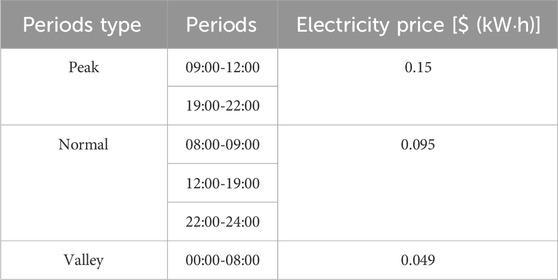
Table 2. Time-of-use price.

To verify the rationality of the proposed model, this article conducts a comparative analysis of the following four cases.

Case 1: Only consider the carbon trading mechanism.

Case 2: Consider DR under the carbon trading mechanism.

Case 3: Only consider DR.

Case 4: Carbon trading mechanism is not considered and DR is not considered.

The optimization results of electric power output for each unit in case 1 are depicted in Figure 2, while the optimization results for heat power output are illustrated in Figure 3. Figure 2 indicates that during the periods (0:00-9:00) and (19:00-24:00), CHP contributes a substantial amount of electricity. In the interval (9:00-16:00), PV contributes significantly, and during (12:00-15:00), the electricity sales volume of the IES increases due to a higher output from CHP and PV. Consequently, the electric energy supplied by WHP is relatively low during the aforementioned time periods, with an increase in WHP output during (19:00-23:00) when CHP and PV outputs are reduced. Figure 3 demonstrates that during the periods (0:00-11:00) and (19:00-24:00), CHP provides a substantial amount of heat power. In the interval (9:00-17:00), owing to the higher output of CHP and PV, GB dominates in providing heat power, serving as a means to absorb excess CHP and PV.

Figure 2

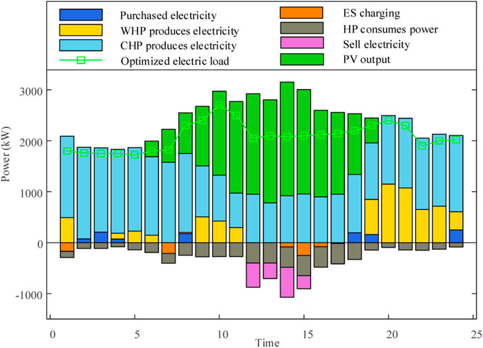
Figure 2. Electric power output in Case 1.

Figure 3

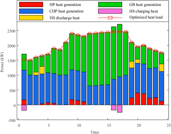
Figure 3. Heat power output in Case 1.

Taking into account CHP, PV output, economic costs, and carbon emissions, the output and costs of each unit are comprehensively considered in Case 2. The optimization results of electric and heat power outputs for each unit during the scheduling period are depicted in Figure 4 and Figure 5. During low-price periods (00:00–08:00), the system relies on CHP, WHP output, and purchased electricity from the higher-level grid to meet the demands of HP, HS charging, and electric loads, maintaining power balance during this period. The heat load is supplied by HP, GB, and HS, achieving heat power balance. ES charges during low-price periods and discharges during high-price periods, while HS operates inversely, enhancing system flexibility. Prioritizing CHP output helps reduce overall operational costs. In Cases where CHP output alone cannot meet the system’s electric load demands and electricity prices are low, the cost of purchasing electricity from the higher-level grid is lower than the cost of purchasing gas from the higher-level gas grid. In cases where HP cannot fully meet the heat load demands, and WHP is inactive during this period, GB is employed for heating during flat electricity price periods (08:00-09:00, 12:00-19:00, 22:00-24:00). During these periods, the system relies on CHP, PV, and WHP output to meet HP and electric load demands, with the heat load supplied by HP and WHP. The electricity prices are relatively higher during these periods, with the cost of purchasing electricity from the higher-level grid exceeding the cost of purchasing gas from the higher-level gas grid. In high-price periods (09:00-12:00, 19:00-22:00), the system relies on CHP, WHP output, and HS discharge to meet HP and electric load demands, with HP and GB supplying the heat load and HS providing heat storage. During these periods, the electricity prices are relatively higher, and purchasing gas from the higher-level gas grid is cheaper than purchasing electricity from the higher-level grid.

Figure 4

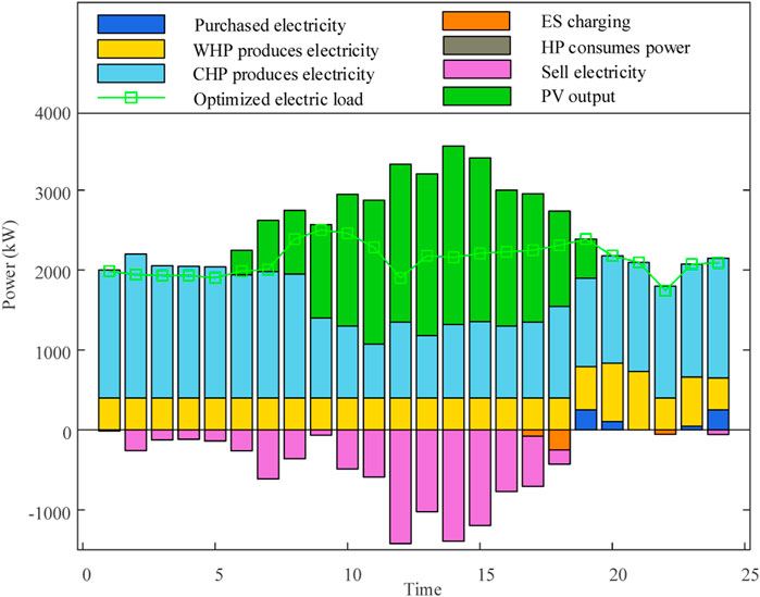
Figure 4. Electric power output in Case 2.

Figure 5

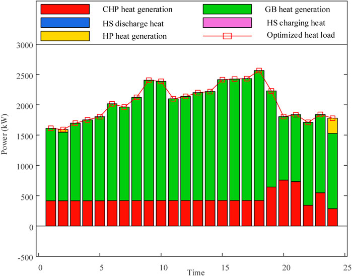
Figure 5. Heat power output in Case 2.

Figure 6 indicates that during the periods of (0:00-8:00) and (19:00-24:00), the IES electric load is primarily supplied by GT, with a lower output from WHP. During the period of (9:00-17:00), the system’s electric load is mainly supported by PV and WP, with no contribution from CHP. During the period of (12:00-15:00), due to the higher output of PV generation, there is surplus system electricity generation, leading to an increase in electricity sales. During the period of (19:00-23:00), when PV generation is inactive, CHP electricity output increases to meet the system’s power demand. Figure 7 illustrates that during the periods of (0:00-10:00) and (18:00-24:00), the GB and HP provide a higher heat power, with lower heat power output from CHP. During the period of (11:00-17:00), due to the higher PV output, there is an abundance of system electricity generation during this period, resulting in a predominant role of HP in producing heat power to absorb excessive PV power.

Figure 6

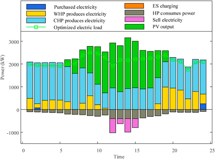
Figure 6. Electric power output in Case 3.

Figure 7

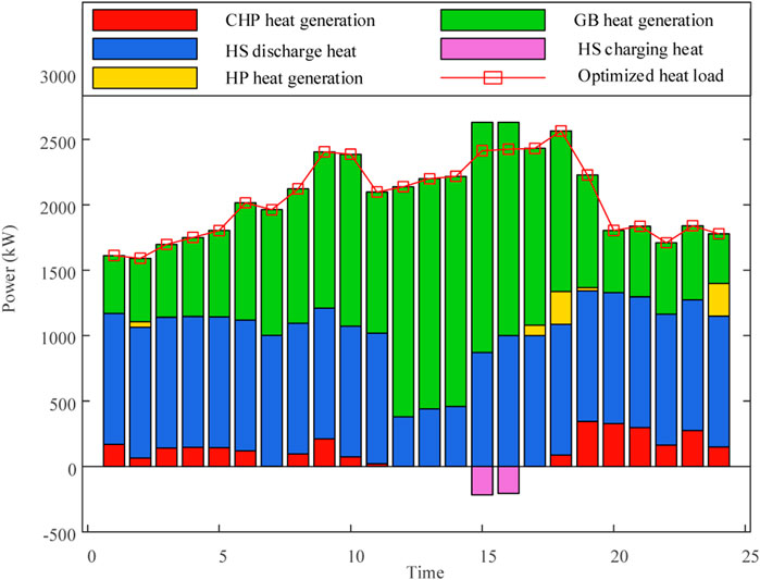
Figure 7. Heat power output in Case 3.

In Case 4, without considering the carbon trading mechanism and DR, depicts the electric and heat outputs of various devices as illustrated in Figure 8 and Figure 9. Figure 8 indicates that, during the period (0:00-5:00), the electric load of the IES is predominantly supplied by CHP, with limited output from ES, necessitating the procurement of electricity from the higher-level grid. In the period (8:00-18:00), the system’s electric load is primarily supported by PV and CHP, with minimal output from CHP. During the period (19:00-24:00), when PV generation is inactive, CHP electric output increases significantly to meet the system’s power demand, leading to a notable increase in purchased electricity. Figure 9 illustrates that, during the period (2:00-11:00), GB and HS contribute a substantial amount of heat power, while CHP heat power output is relatively low. In the period (12:00-17:00), the system’s heat power is mainly borne by GB and HS, with HS contributing the majority of the heat production.

Figure 8

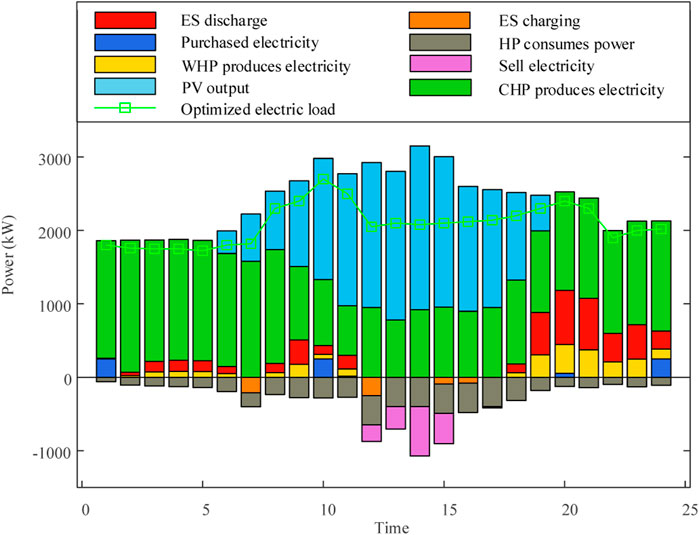
Figure 8. Electric power output in Case 4.

Figure 9

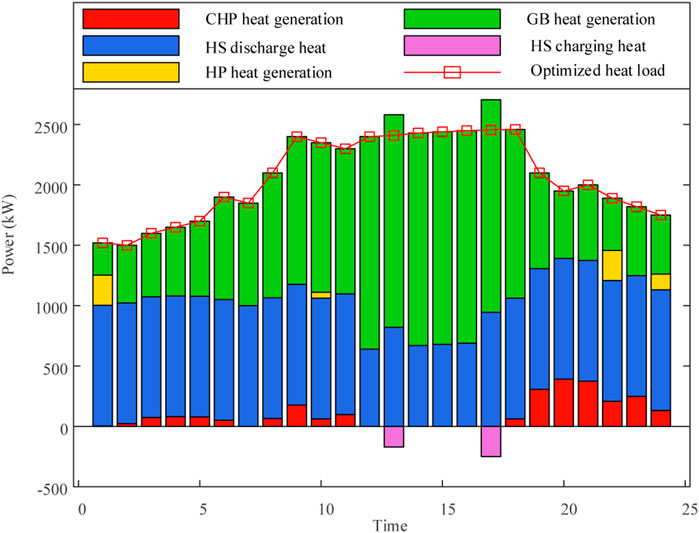
Figure 9. Heat power output in Case 4.

The costs and actual carbon emissions of each scenario are shown in Table 3. Compared with Case 4, the carbon emission cost of Case 1 has decreased by 77.89%, with an actual reduction in carbon emissions of 4877.08 kg. This outcome is attributed to the consideration of a carbon emission mechanism in Case 1, which endows the system with initial carbon emission quotas, thereby offsetting a portion of the carbon emission costs. In contrast, Case 4 necessitates the consideration of the total cost associated with the actual carbon emissions. In comparison to Case 4, the energy procurement cost in Case 3 has decreased by 10.25%. This reduction is attributed to the incorporation of DR, which reduces peak electricity demand while increasing off-peak electricity demand. Consequently, the system can opt for a more economical energy procurement method. Compared with Cases 1 and 2, Case three exhibits higher total operational costs, lower energy procurement costs, and higher carbon trading costs and actual carbon emissions. This observation underscores the promotive role of carbon trading mechanisms in energy conservation and emission reduction. Case 2 demonstrates lower total operational costs, energy procurement costs, carbon trading costs, operational maintenance costs, and actual carbon emissions than Case 1. This outcome is attributed to the consideration of DR under the carbon trading mechanism, which not only shifts a portion of the load from high electricity price periods to low electricity price periods but also reduces energy consumption during certain load conditions. Furthermore, the mechanism facilitates the mutual substitution of electric and heat energy on the consumer side, smoothing the load curve. Consequently, the system, by comparing the costs of purchasing electricity and gas at different time periods and the outputs of GT and GB, selects an economically and environmentally favorable operational mode. This approach effectively coordinates the economic efficiency and low-carbon nature of the system’s operation.

Table 3

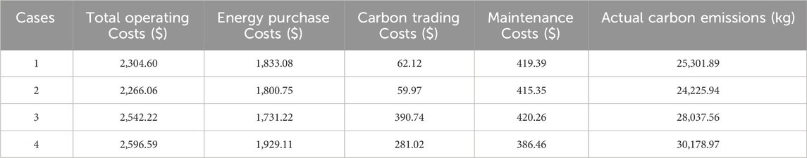
Table 3. Daily operation cost in 4 cases.

5 Conclusion

This study establishes an optimized operational model considering DR under the carbon trading mechanism for integrated energy systems. The impact of carbon trading prices on system operation is investigated with set four cases. The conclusions are as follows.

1) Under the carbon trading mechanism, considering DR not only shifts a portion of the load from high electricity price periods to low electricity price periods and reduces load energy consumption but also achieves the mutual substitution of electric and heat energy on the user side, smoothing the load curve.

2) Considering that the ladder carbon trading mechanism system with an initial carbon emission allowance, the operating cost of the system is reduced.

Data availability statement

The data analyzed in this study is subject to the following licenses/restrictions: To confidentiality requirements, the dataset will not be made public. Requests to access these datasets should be directed to JL, jing20180806@163.com.

Author contributions

JL: Writing–original draft, Conceptualization. XG: Writing–review and editing, Data curation. DG: Writing–review and editing, Investigation. JX: Writing–review and editing, Project administration. ZJ: Writing–review and editing, Resources. YW: Writing–review and editing, Supervision.

Funding

The author(s) declare that financial support was received for the research, authorship, and/or publication of this article. This work was supported by Science and Technology Project of State Grid Liaoning Electric Power Supply Co., Ltd. (SGLNYX00DFJS2310107). The funder was not involved in the study design, collection, analysis, interpretation of data, the writing of this article, or the decision to submit it for publication.

Conflict of interest

The authors declare that this study received funding from State Grid Liaoning Electric Power Supply Co., Ltd.. The funder was not involved in the study design, collection, analysis, interpretation of data, the writing of this article, or the decision to submit it for publication.

Publisher’s note

All claims expressed in this article are solely those of the authors and do not necessarily represent those of their affiliated organizations, or those of the publisher, the editors and the reviewers. Any product that may be evaluated in this article, or claim that may be made by its manufacturer, is not guaranteed or endorsed by the publisher.

References

Ceseña, E., and Mancarella, P. (2019). Energy systems integration in smart districts: robust optimisation of multi-energy flows in integrated electricity, heat and gas networks. IEEE Trans. Smart Grid 10 (1), 1122–1131. doi:10.1109/tsg.2018.2828146

CrossRef Full Text | Google Scholar

Chen, X., Lv, J., McElroy, M. B., Han, X., Nielsen, C. P., and Wen, J. (2018). Power system capacity expansion under higher penetration of renewables considering flexibility constraints and low carbon policies. IEEE Trans. Power Syst. 33 (6), 6240–6253. doi:10.1109/tpwrs.2018.2827003

CrossRef Full Text | Google Scholar

Cheng, Y., Zhang, N., Wang, Y., Yang, J., Kang, C., and Xia, Q. (2019). Modeling carbon emission flow in multiple energy systems. IEEE Trans. Smart Grid 10 (4), 3562–3574. doi:10.1109/tsg.2018.2830775

CrossRef Full Text | Google Scholar

Clegg, S., and Mancarella, P. (2016). Integrated electrical and gas network flexibility assessment in low-carbon multi-energy systems. IEEE Trans. Sustain. Energy 7 (2), 718–731. doi:10.1109/tste.2015.2497329

CrossRef Full Text | Google Scholar

Correa-Posada, C. M., and Sanchez-Martin, P. (2015). Integrated power and natural gas model for energy adequacy in short-term operation. IEEE Trans. Power Syst. 30 (6), 3347–3355. doi:10.1109/tpwrs.2014.2372013

CrossRef Full Text | Google Scholar

Fang, J., Zeng, Q., Ai, X., Chen, Z., and Wen, J. (2018). Dynamic optimal energy flow in the integrated natural gas and electrical power systems. IEEE Trans. Sustain. Energy 9 (1), 188–198. doi:10.1109/tste.2017.2717600

CrossRef Full Text | Google Scholar

Good, N., and Mancarella, P. (2019). Flexibility in multi-energy communities with electrical and thermal storage: a stochastic, robust approach for multi-service demand response. IEEE Trans. Smart Grid 10 (1), 503–513. doi:10.1109/tsg.2017.2745559

CrossRef Full Text | Google Scholar

Khani, H., and Farag, H. E. Z. (2018). Optimal day-ahead scheduling of power to-gas energy storage and gas load management in wholesale electricity and gas markets. IEEE Trans. Sustain. Energy 9 (2), 940–951. doi:10.1109/tste.2017.2767064

CrossRef Full Text | Google Scholar

Li, F., Qin, J., and Kang, Y. (2020). Closed-loop hierarchical operation for optimal unit commitment and dispatch in microgrids: a hybrid system approach. IEEE Trans. Power Syst. 35 (1), 516–526. doi:10.1109/tpwrs.2019.2931293

CrossRef Full Text | Google Scholar

Li, G., Zhang, R., Jiang, T., Chen, H., Bai, L., and Li, X. (2017). Security-constrained bi-level economic dispatch model for integrated natural gas and electricity systems considering wind power and power-to-gas process. Appl. Energy 194, 696–704. doi:10.1016/j.apenergy.2016.07.077

CrossRef Full Text | Google Scholar

Li, Y., Liu, M., Wen, W., Wen, F., Wang, K., and Huang, Y. (2018). Optimal operation strategy for integrated natural gas generating unit and power-to-gas conversion facilities. IEEE Trans. Sustain. Energy 9 (4), 1870–1879. doi:10.1109/tste.2018.2818133

CrossRef Full Text | Google Scholar

Liotta, G., Kaihara, T., and Stecca, G. (2016). Optimization and simulation of collaborative networks for sustainable production and transportation. IEEE Trans. Ind. Inf. 12 (1), 417–424. doi:10.1109/tii.2014.2369351

CrossRef Full Text | Google Scholar

Saboori, H., and Hemmati, R. (2016). Considering carbon capture and storage in electricity generation expansion planning. IEEE Trans. Sustain. Energy 7 (4), 1371–1378. doi:10.1109/tste.2016.2547911

CrossRef Full Text | Google Scholar

Saboori, H., and Hemmati, R. (2018). Considering carbon capture and storage in electricity generation expansion planning. IEEE Trans. Sustain. Energy 7 (4), 1371–1378. doi:10.1109/tste.2016.2547911

CrossRef Full Text | Google Scholar

Shang, Y., and Li, S. (2024). FedPT-V2G: security enhanced federated transformer learning for real-time V2G dispatch with non-IID data. Appl. Energy 358, 122626. doi:10.1016/j.apenergy.2024.122626

CrossRef Full Text | Google Scholar

Shang, Y., Yu, H., Shao, Z., and Jian, L. (2022). Achieving efficient and adaptable dispatching for vehicle-to-grid using distributed edge computing and attention-based LSTM. IEEE Trans. Ind. Inf. 18 (10), 6915–6926. doi:10.1109/tii.2021.3139361

CrossRef Full Text | Google Scholar

Shao, C., Wang, X., Shahidehpour, M., Wang, X., and Wang, B. (2017). An MILP-based optimal power flow in multicarrier energy systems. IEEE Trans. Sustain. Energy 8 (1), 239–248. doi:10.1109/tste.2016.2595486

CrossRef Full Text | Google Scholar

Wang, Y., Qiu, J., Tao, Y., and Zhao, J. (2020). Carbon-oriented operational planning in coupled electricity and emission trading markets. IEEE Trans. Power Syst. 35 (4), 3145–3157. doi:10.1109/tpwrs.2020.2966663

CrossRef Full Text | Google Scholar

Yang, J., Zhang, N., Yao, H., Kang, C., and Xia, Q. (2019). Modeling the operation mechanism of combined P2G and gas-fired plant with CO₂ recycling. IEEE Trans. Smart Grid 10 (1), 1111–1121. doi:10.1109/tsg.2018.2849619

CrossRef Full Text | Google Scholar

Zhou, B., Xu, D., Cao, Y., Chan, K. W., Xu, Y., et al. (2018). Multiobjective generation portfolio of hybrid energy generating station for mobile emergency power supplies. IEEE Trans. Smart Grid 9 (6), 5786–5797. doi:10.1109/tsg.2017.2696982

CrossRef Full Text | Google Scholar

Zhou, Y., Wei, H., Yong, M., and Dai, Y. (2019). Integrated power and heat dispatch considering available reserve of combined heat and power units. IEEE Trans. Sustain. Energy 10 (3), 1300–1310. doi:10.1109/tste.2018.2865562

CrossRef Full Text | Google Scholar

Nomenclature