A stochastic power flow-based static security assessment under uncertain scenarios

With the gradual increase in the grid-connected capacity of renewable energy sources, the uncertainty in the operation of power systems has increased, posing challenges to static security assessment considering N-1 contingency scanning. To address this, this article first establishes a static security calculation model based on stochastic power flow. Then, it proposes stochastic component-level safety indexes and system-level safety indexes. Finally, using the analytic hierarchy process to analyze the obtained weighting coefficients, the article establishes a system of static security assessment indexes for power systems. A data-driven simulation method based on extreme gradient boosting (XGBoost) is proposed to tackle the high time consumption of multi-scenario static security assessment, which brings difficulties in model debugging and application. Case studies based on the IEEE 39-bus system demonstrate the effectiveness of the proposed model and the rapidity of the data-driven approach.

1 Introduction

As the operational environment of the power grid evolves, the system faces increasing random disturbances, leading to more complex and variable conditions. However, the traditional static security assessment (SSA) for N-1 contingency scanning has difficulty dealing with the increasing uncertainties (Čepin, 2011; Chen et al., 2015; Meegahapola et al., 2020; Qian et al., 2022). To ensure the system’s safety and stability, it is crucial to develop a stochastic-based SSA method.

The primary feature of an electrical power system is to ensure the reliability, cost-effectiveness, and quality of the power supply, providing continuous and uninterrupted energy to users (Das, 2007; Schavemaker and Van der Sluis, 2017). Power system safety analysis is categorized into static and dynamic safety analyses. SSA assumes that the power system transitions directly from a pre-disturbance static state to a post-disturbance static state without considering the intermediate transient processes. This analysis is used to verify whether various constraints are satisfied following a disturbance (Prabhakar et al., 2022). Dynamic safety analysis, on the other hand, examines the power system’s ability to maintain stability during the transient process from a pre-disturbance static state to a post-disturbance static state (Rao et al., 2009).

By considering the randomness of wind power and PV power generation, the accuracy of the static safety evaluation method can be improved, thereby providing a more reliable safety reference and ensuring that the system can cope with emergencies and failures. Accurate static safety evaluation can assist decision makers in formulating more effective scheduling strategies and emergency plans to improve the reliability and safety of the power system. Power system static security assessments have been widely investigated in previous studies. The existing methods can be classified as i) model based, ii) signal-based, and iii) artificial intelligence (AI) (Wu, 2015). The model-based methods use a mathematical expression of the power system to analyze the security status (Jing, 2014). The main disadvantages of model-based methods are that it is difficult to provide an accurate model for the power system in most cases, and models are unsuitable for real-time assessment based on accurate modeling. Signal-based methods have better calculation accuracy, but they depend on a predefined threshold and are notably sensitive to the completeness of the information about the power system’s status. AI-based methods require historical data to assess the power system security status. The main methods include random forest (Wang et al., 2016), multi-class support vector machine (SVM) (Meegahapola et al., 2020), core vector machine (Mohammadi et al., 2010), etc. These methods are restricted in terms of extracting the comprehensive features in complex and nonlinear systems such as power networks.

Load flow analysis is crucial for power system SSA; it can address the load uncertainties from forecasting errors and operational conditions, particularly with renewable energy integration (Kalyani and Swarup, 2010; Afrasiabi et al., 2019). Stochastic load flow offers statistical insights into node voltages and branch powers, facilitating the evaluation of random factors and probability distributions at specific operational points (Shirasaki and Uchida, 2010). There are three general methods used for stochastic power flow calculation: simulation, analytical, and approximate approaches (Su, 2005; Wang et al., 2008; Ghiasi, 2018). Monte Carlo simulation generates a stochastic process to approximate solutions by analyzing statistical properties (Binder et al., 1992; Conti and Raiti, 2007; Thomopoulos, 2012; Graham and Talay, 2013). The analytical method uses simplified DC and AC load flow equations with convolution techniques to calculate output distributions based on input variables, effectively modeling stochastic behavior under varying conditions (Hu and Wang, 2007; Kiruthika and Bindu, 2020; Han et al., 2021). The approximate method estimates system state variables’ statistical characteristics from input variables’ statistical features, reducing computational demands. It is ideal for quick assessments (Morales and Perez-Ruiz, 2007). These methods are essential for power generation planning, network planning, SSA, real-time operational state analysis, optimal load flow calculations, and risk assessments, especially as power systems face rising uncertainties.

In summary, the prevailing research on N-1 security scanning predominantly utilizes deterministic load flow analysis, which does not adequately account for the stochastic variations introduced by wind and solar energy sources. By taking uncertainties into account, the article proposes a novel static security assessment methodology that leverages stochastic load flow simulation and incorporates a data-driven acceleration algorithm, addressing the complexities of static security assessment in the face of stochastic variations effectively.

The organization of the subsequent sections of this article is as follows: Section 2 establishes a static security index system that considers stochasticity and develops a stochastic load flow model based on simulation methods. Section 3 introduces a data-driven method for stochastic static security assessment. Section 4 provides a case study analysis based on the IEEE 39-bus system. Section 5 concludes the article.

2 Model formulation

The model formulation process is as follows: Initially, it establishes probability distribution models for load, photovoltaic (PV), and wind power, generating random scenarios with uncertainty. Then, it calculates the DC optimal power flow, using the result as the base case for power flow. Following the base case flow, the Newton–Raphson method is employed to compute the stochastic load flow for the generated probability distribution scenarios. Finally, it utilizes a kernel density estimation (KDE) algorithm to fit the results of the stochastic load flow calculations.

2.1 Stochastic power flow model

2.1.1 Model for uncertainty sources

(1) Load Probability Model

In most stochastic load flow studies, load uncertainty is assumed to be normally distributed, with the power injections at nodes being either independent or linearly related (Tuinema et al., 2020). Based on this, this article develops a stochastic model for the active and reactive power of system loads that adhere to a normal distribution.

There is always a deviation in load forecasting, expressed as: $P_D=\overline{P_D}+\Delta P_D$, where $\Delta P_D$ is the load forecast error random variable. $\overline{P_D}$ is the load forecast error. $\Delta P_D$ is the load forecast deviation, which follows a normal distribution with a mean of 0 and a variance of ${\sigma }_D^2$. The calculation formula for the variance is:

${\sigma }_D^2=\frac{\overline{P_D}\zeta }{100}$

The probability density function of the load forecast error random variable as follows:

$f=\frac{1}{\sqrt{2\pi }\sigma }\cdot \mathit{exp}\left[-\frac{{\left(P-\mu \right)}^2}{2{\sigma }^2}\right]$

where $\sigma$ represents the standard deviations of active and reactive power; $\mu$ represents the means of active and reactive power.

(2) Photovoltaic and Wind Power Plant Probability Model

We can describe the uncertainty of PV and wind power output by superimposing the forecast error $\epsilon$ onto the predicted value $P$ (Al-Sumaiti et al., 2019). The PV and wind power output can be represented as:

$P^{*}=P+\epsilon$

The standard deviation of power forecast error $\epsilon$ is normally distributed. It has a mean of zero. The standard deviation is $\sigma$, and its probability density function is:

$f\left(\epsilon \right)=\frac{1}{\sqrt{2\pi }\sigma }\cdot \mathit{exp}\left[-\frac{{\epsilon }^2}{2{\sigma }^2}\right]$

where $\sigma$ is proportional to the predicted output.

2.1.2 Stochastic power flow model

The article initially addresses the solution of the DC optimal power flow, employing the outcome as the base case for power flow. Thereafter, the Newton–Raphson method is utilized to compute the system’s stochastic load flow, establishing the stochastic power flow model.

For a combined generation and transmission system with $n$ nodes and $b$ lines, the DC optimal power flow model can be written as follows:

$f_P=min\left\{{\displaystyle \sum _{i\in NL}}{P}_{Ci}\right\}$

The following constraints should be satisfied:

${\displaystyle \sum _{i\in NG}}{\displaystyle \sum _j}{P}_{G_{ij}}+{\displaystyle \sum _{i\in NL}}{P}_{C_i}={\displaystyle \sum _{i\in NL}}{P}_{L_i}$

$P_G+P_C-P_L=-Y\theta$

$P_{bi}=\frac{{\theta }_{s\left(i\right)}-{\theta }_{e\left(i\right)}}{x_i}\left(i\in NT\right)$

$\left|P_b\right|\le \overline{P_b}$

${\underset{¯}{P_G}}_{ij}\le {P_G}_{ij}\le \overline{{P_G}_{ij}}$

$P_C\le P_L$

$P_C\ge 0$

$-P_r^{\mathit{max}}\left(t\right)\le P\left(t\right)-P\left(t-1\right)\le P_r^{\mathit{max}}\left(t\right)$

${\displaystyle \sum _{i\in NL}}{R}_i\left(t\right)\ge R_S\left(t\right)$

$0\le R_i\left(t\right)\le \overline{R_i}$

where $f_P$ is the objective function value in optimization calculation, and $P_{Ci}$ and $P_{L_i}$ are the active power load cut and active power load at bus $t$. ${P_G}_{ij}$, $\overline{{P_G}_{ij}}$ and $\underset{\_}{{P_G}_{ij}}$ represent the active power output, the upper limit, and the lower limit of the active power output for the jth unit at the ith generator bus. $P_G$, $P_C$, $P_L$, and $\theta$ is an n-dimensional column vector. It includes elements for active power injections at independent nodes, active power load shed, active power load, and node voltage angles. Matrix $Y$ is the node admittance matrix. It is built using the inverse of line reactance as branch admittances. $P_b$ is a b-dimensional column vector. Its elements $P_{bi}$ represent the active power flow in line $i$. $s\left(i\right)$ and $e\left(i\right)$ are the node numbers of the starting and ending nodes of line $i$, and $x_i$ is the reactance of line $i$. $\overline{P_b}$ is a b-dimensional column vector. Its elements represent the active power capacity of lines. Sets $NL$, $NG$, and $NT$ represent the load bus set, generation bus set, and line set. $P_r^{\mathit{max}}\left(t\right)$ denotes the maximum ramp-up or ramp-down power of the unit per hour. $R_i\left(t\right)$ is the spinning reserve provided by load bus $i$ at time $t$. $R_s\left(t\right)$ is the spinning reserve requirement of the system at time $t$. $\overline{R_i}$ is the maximum spinning reserve that generation bus $i$ can provide.

The stochastic load flows have been calculated based on the solved DC base case power flow. The probability distribution models for node voltage $U$ and branch power flow $Z$ are as follows:

$\begin{array}{c}U=g\left(S\right)\\ Z=h\left(S\right)\end{array}$

where $g$ and $h$ represent the node voltage function and branch power flow function.

Subsequently, the Newton–Raphson method is used to solve the stochastic load flow based on the generated probability distribution models. This approach yields the system power flow distribution results for each random case. Further, the KDE algorithm is used to fit the probability distribution of output data.

Given $d$ load data samples from $n$ hours at load nodes, the load vector for the ith hour can be represented as $X_i={\left[X_{i1},X_{i2},...,X_{in}\right]}^T$. If we choose the Gaussian function as the kernel for kernel density estimation, then the multi-dimensional kernel density estimate takes the following form:

$f\left(X\right)=\frac{1}{n}{\displaystyle \sum _{i=1}^n}\frac{\mathit{exp}\left(-\frac{{\left(x-X_i\right)}^T{H}^{-1}\left(x-X_i\right)}{2}\right)}{{\left(2\pi \right)}^{d/2}\mathit{det}{\left(H\right)}^{1/2}}$

where $n$ is the size of the historical sample. $\mathit{det}$ represents the determinant calculation. It can be seen that $f\left(X\right)$ contains $n$ d-dimensional Gaussian kernels, with the mean of the ith kernel being $X_i$. $H$ is the bandwidth matrix.

2.2 N-1 static security assessment indexes

The impact of random disturbances or faults on power systems primarily manifests as branch overloads and node voltage violations: branch overloads may trigger cascading failures, while node voltage violations may lead to voltage collapse (De La Ree et al., 2005; Ibrahim, 2011). Therefore, the SSA of the system is conducted mainly from two aspects: branch overloads and node voltage violations. The assessment perspective involves two levels: safety risk and safety probability.

2.2.1 Component-level safety index

(1) Severity Index

The load flow percentage of each line determines the degree of overload.

${Sev}_{branch}\left(K_{P_j}\left|E\right.\right)={\sum }_{k=1}^K\mathit{max}\left\{\frac{\left|P_j\right|-\left|P_{\mathit{max}}\right|}{\left|P_{\mathit{max}}\right|},\frac{\left|P_j\right|-\left|P_{\mathit{min}}\right|}{\left|P_{\mathit{min}}\right|}\right\}$

where $E$ represents the set of all possible contingencies. $K_{Pj}$ denotes the event of branch $j$ exceeding its power flow limit. $P_{\mathit{max}}$ and $P_{\mathit{min}}$ represents the maximum and minimum active power value allowed to be transmitted on branch $j$.

The node voltage severity function typically defines the percentage deviation of each node voltage magnitude from its normal magnitude limit.

$Se{v}_{voltage}\left(\left.K_{v_i}\right|E\right)={\displaystyle \sum _{k=1}^K}\mathit{max}\left\{\frac{v_H-v_i}{v_H},\frac{v_i-v_L}{v_i}\right\}$

(2) Component failure probability

The probability that the network operation fails to meet the power flow security constraints after a specific anticipated event occurs can be determined as follows:

$\mathit{Pr}\left(\left.K_{v_i}\right|E\right)=prob\left\{v_L<\left|v_i\right|<v_H\right\}=F_{v\theta }\left(\frac{v_H-v_i}{{\sigma }_{vi}}\right)-F_{v\theta }\left(\frac{v_L-v_i}{{\sigma }_{vi}}\right)$

where $K_{v_i}$ represents the event of no voltage violation at node $v_i$. $E$ represents the set of all fault events. $v_i$ and $v_H$ represents the upper and lower limits of the safe voltage range.

The probability that branch $j$ does not exceed its power flow limit is expressed as:

$Pr\left(\left.K_{P_i}\right|E\right)=prob\left\{-P_{\mathit{max}}<P_j<P_{\mathit{max}}\right\}=F_{pq}\left(\frac{P_{\mathit{max}}-P_j}{{\sigma }_{pj}}\right)-F_{pq}\left(\frac{{-P}_{\mathit{max}}-P_j}{{\sigma }_{pj}}\right)$

where $K_{P_i}$ represents the event of no power flow violation on branch $j$. $P_{\mathit{max}}$ is the upper limit of the branch power flow.

2.2.2 System-level safety indexes

The system risk or insecurity probability is a comprehensive reflection of the risks or insecurity probabilities of individual components.

(1) System Risk Index

The system overload severity index is defined as:

$R_{OL}=\alpha \frac{1}{M}{‖Se{v}_{branch}‖}_1+\beta {‖Se{v}_{branch}‖}_{\infty }$

where $\alpha$ and $\beta$ are weighting coefficients, satisfying $\alpha +\beta =1$. ${‖Se{v}_{branch}‖}_1$ and ${‖Se{v}_{branch}‖}_{\infty }$ represent the 1 and ∞ norms of vector $R$, respectively.

The system voltage violation severity index is defined as:

$R_{OV}=\alpha \frac{1}{N}{‖Se{v}_{voltage}‖}_1+\beta {‖Se{v}_{voltage}‖}_{\infty }$

(2) System probability indexes

The failure of component $i$ can be expressed as:

$E_i={\overline{F}}_1\cap {\overline{F}}_2...{\overline{F}}_{i-1}\cap F_i\cap {\overline{F}}_{i+1}...{\overline{F}}_N$

where $F_i$ represents the failure state of the component. ${\overline{F}}_i$ represents the normal state of the component, and $N$ is the number of components.

Furthermore, the probability that the system satisfies power flow security constraints after an anticipated event occurs is given by:

$\mathit{Pr}\left(\left.K_0\right|E_i\right)=\left({\displaystyle \prod _{i=1}^n}\mathit{Pr}\left(\left.K_{v_i}\right|E_i\right)\right)\left({\displaystyle \prod _{j=1}^m}\mathit{Pr}\left(\left.K_{p_j}\right|E_i\right)\right)$

The probability that the system does not satisfy power flow security constraints is given by:

$\mathit{Pr}\left(\left.K_1\right|E_i\right)=1-\mathit{Pr}\left(\left.K_0\right|E_i\right)$

where $K_1$ represents the event of the system satisfying power flow security constraints. $K_0$ represents the event of the system not satisfying power flow security constraints. $E_i$ represents the event of a specific accident occurring in the system.

Assuming the probability of component $i$ failing at time $t$ follows a Poisson distribution, and events occur independently of one another, it has:

$\mathit{Pr}\left(E_i\right)=\left(1-e^{-{\lambda }_{i}t}\right)\mathit{exp}\left(-{\displaystyle \sum _{j\ne i}}{\lambda }_{j}t\right)$

where ${\lambda }_j$ is the failure rate of component $i\left(i=1,2,\dots ,N\right)$.

Then, the probability of power flow security for the system is obtained as:

${\mathit{Pr}}_s={\mathit{Pr}}_{s0}\cdot \left(1-{\displaystyle \sum _{k=1}^N}p{r}_{E_k}\right)+{\displaystyle \sum _{k=1}^N}p{r}_{sk}\cdot p{r}_{E_k}$

The probability of power flow insecurity for the system is given by:

${\mathit{Pr}}_{ins}=1-{\mathit{Pr}}_s$

In this subsection, this article integrates the subjective weighting model constructed using the analytic hierarchy process (AHP) (Chatzimouratidis and Pilavachi, 2007) and the objective weighting model constructed using the entropy method using the additive integration method.

First, the proportions of each weight are determined in the comprehensive weights:

$y={\displaystyle \sum _{i=1}^n}\left(k_1{p}_i+k_2{q}_i\right)x_i$

where $p_i$ and $q_i$ respectively denote the subjective and objective weights of the ith indexes. $k_1$ and $k_2$ are undetermined coefficients, and $k1+k2=1,k1,k2>0$. $n$ represents the number of indexes being evaluated.

Next, the formula for calculating the comprehensive weight coefficient of the ith index is given as follows:

$\begin{array}{cc}{w}_i=k_1{p}_i+k_2{q}_i& \left(i=1,2,3,\dots ,n\right)\end{array}$

The overall system static security assessment index S₀ is obtained as follows:

$S_0=w_1\cdot {\mathit{Pr}}_{ins}+w_2\cdot R_{OL}+w_3\cdot R_{OV}$

3 Data-driven static security assessment algorithm

Considering the issues of long training times and the difficulty of extracting features from data in data-driven models, this article employs the XGBoost method to reduce the simulation time and application complexity in the safety assessment of power systems.

Initially, this article uses the Monte Carlo simulation method to construct random scenarios reflecting the stochastic fluctuations in load, PV, and wind output values. Following this, an iteration through all fault conditions of lines and generators is conducted. The method can solve the corresponding random scenarios for each fault condition. Subsequently, the static unsafety indexes for the system under the respective fault conditions are calculated, applying the method detailed in Section 2.2.

XGBoost is a machine learning algorithm based on tree models (Chen and Guestrin, 2016), which automatically selects appropriate splitting directions when samples are missing, making it suitable for processing tabular data. First, the system safety assessment scenario is designed, the fault set and data collection points are selected, and the sample set that characterizes the random power flow input and output changes under normal operation and fault conditions is constructed as follows:

$\mathbf{X}=\left[X_1,\dots ,X_i,\dots ,X_N\right]\in R^{N\times M}$

where N represents the number of samples, that is, N safety assessment scenarios, and M represents the dimension of each sample feature vector. The input feature vector of sample $X_i$ contains the mean $\left\{f_h|h\in H\right\}$ and variance $\left\{{\sigma }_h|h\in H\right\}$ of the branch active power flow distribution $\left\{f_h|h\in H\right\}$ and the amplitude $\left\{{\nu }_a|a\in A\right\}$ and variance $\left\{{\epsilon }_a|a\in A\right\}$ of the node voltage. The dimension M is the sum of the number of branches and the number of nodes A. The system insecurity probability $y_i$ corresponding to each sample $X_i$ constitutes the output of the data-driven model.

Based on the new energy power system safety assessment data set established, K classification and regression trees are selected as base learners; further, based on the regression idea of the boosting method, the sample data is input into the XGBoost model, and the output vectors of multiple base learners are continuously added as the tree model of XGBoost. Finally, the learned system insecurity probability can be obtained by using the $Soft\max$ function. The training flow chart is shown in Figure 1.

Figure 1

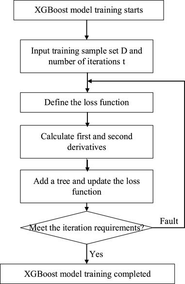
Figure 1. XGBoost model training flow chart.

Based on the renewable energy power system static security assessment dataset established, K classification and regression trees are chosen as base learners. The learned system insecurity probability can be obtained by utilizing the cumulative function. The system static security assessment framework is illustrated in Figure 1, and for a given dataset $D=\{\left.\left(X_i,y_i\right)\right\}\left(\left|D\right|=N,X_i\in R^M,y_i\in R\right)$, the ensemble model of trees is represented by the following equation:

${\widehat{y}}_i={\displaystyle \sum _{k=1}^K}{T}_k\left(X_i\right),T_k\in \mathrm{\Gamma }$

In the equation, ${\widehat{y}}_i$ represents the output of the model. $T_k\left(X_i\right)$ denotes the prediction result of the kth decision tree. $T\left(x\right)={\varpi }_{q\left(x\right)}$ represents the mapping from the input sample to the leaf node of the kth tree; each tree corresponds to an independent tree structure $T_k$ and the weights of the leaves $\varpi$. $X_i$ is the feature vector of the ith sample. $X_i$ represents the mapping of the structure of the kth tree to the leaf corresponding to the sample. $\mathrm{\Lambda }$ is the number of leaves on the tree; $\mathrm{\Gamma }=\left\{T\left(x\right)={\varpi }_{q\left(x\right)}\right\}\left(q:R^m\to \mathrm{\Lambda },\varpi \in R^{\mathrm{\Lambda }}\right)$ is the collection space of trees.

The objective function trained by XGBoost can be represented as:

$obj\left(\phi \right)={\displaystyle \sum _{i=1}^n}l\left(y_i,{\widehat{y}}_i\right)+{\displaystyle \sum _{k=1}^K}\mathrm{\Omega }\left(T_k\right)={\displaystyle \sum _{i=1}^n}l\left(y_i,{\widehat{y}}_i+{\mathrm{\Gamma }}_i\left(X_i\right)\right)+\mathrm{\Omega }\left(T_k\right)+C$

where $\phi$ represents the model parameters. ${\displaystyle \sum _{i=1}^N}l\left(y_i,{\widehat{y}}_i\right)$ denotes the quantified error of the model on the training samples. $N$ is the number of training samples. ${\displaystyle \sum _{k=1}^K}\mathrm{\Omega }\left(T_k\right)$ is the regularization term of model complexity used to reduce the risk of overfitting. $K$ is the number of base learners of the model.

In the XGBoost algorithm, the model complexity of a single base learner is defined as:

$\mathrm{\Omega }\left(T_k\right)=\gamma M+\frac{1}{2}\lambda {\displaystyle \sum _{j=1}^M}{‖{\varpi }_j‖}^2$

where $M$ represents the number of leaf nodes in the base learner. $\lambda$ denotes the $L_2$ regularization coefficient. $\gamma$ represents the difficulty of node splitting. ${‖{\varpi }_j‖}^2$ denotes the norm of the leaf node weights.

Based on the established dataset for assessing the security of new energy power systems (shown in Figure 2), CART base learners are continuously trained to fit the residuals of the previous model and then integrated into the XGBoost model. Iteration continues until either the preset number of base learners is trained or the model residuals are smaller than the set threshold.

${\widehat{y}}_i^{\left(0\right)}=0$

$\cdots$

${\widehat{y}}_i^{\left(t\right)}={\displaystyle \sum _{k=1}^t}{T}_k\left(x_i\right)={\widehat{y}}_i^{\left(t-1\right)}+T_k\left(x_i\right)$

where ${\widehat{y}}_i^{\left(t\right)}$ represents the model prediction value for the ith sample in the tth round, with the model prediction values from the previous tth rounds retained before adding a new function $T_t\left(X_i\right)$.

Figure 2

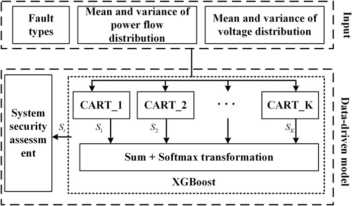
Figure 2. System security assessment framework.

4 Case study

In the case study, the SSA indexes for a system postulated are assessed with accidents detailed. This includes evaluating the likelihood that voltage and power flow limits are not exceeded after each accident, considering uncertainties in power injections and line failures. The study calculates the overall system safety by integrating these probabilities with the frequency of each pre-planned accident.

Then, fault scenarios for the case are constructed. The average failure probability for units is 1×10⁻⁴ times/hour, with the range from 5 × 10⁻⁵∼2 × 10⁻⁴. The average failure probability for branches is 1.2 × 10⁻⁴ times/hour, with the range from 2 × 10⁻⁵∼2 × 10⁻⁴. The transmission capacity of all branches is consistent with the IEEE 39-bus case, and the transmission capacity limit during emergencies is 2.5 times that of normal conditions.

4.1 Model-driven analysis

(1) Component and System Safety Index Ranking Analysis

By ranking the items in the safety function according to the calculation results, the links that contribute significantly to the overall probability of system unsafety can be identified, drawing attention to them. Figure 3 provides risk indexes for each component in the system under various fault occurrence probabilities. For each unit, this reflects the risk of a voltage limit violation at the node where the unit is located. For each branch, it reflects the risk of a power flow limit violation on that branch. The higher the risk index, the greater the threat to the system in the event of a fault at that node or on that branch.

Figure 3

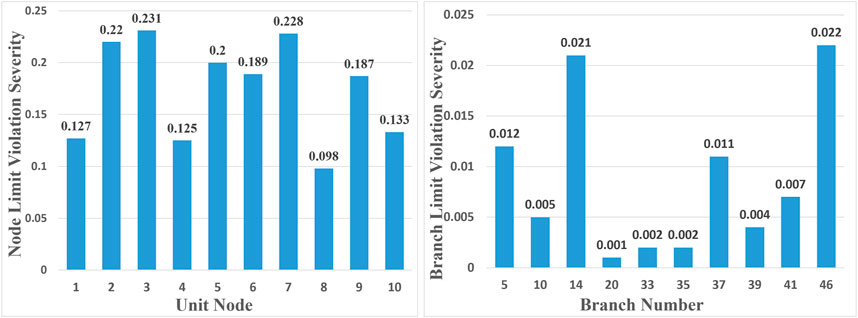
Figure 3. Component unsafe severity.

Additionally, by ranking the probabilities of the system not meeting power flow safety constraints for each pre-planned accident, the fault items that most affect the probability of system power flow can be identified. More targeted preventive measures can be implemented. Figure 4 provides the probabilities of system unsafety caused by the failure of each component, considering the failures of various components.

(2) System Safety Assessment Simulation Analysis

Figure 4

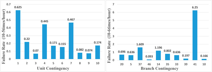
Figure 4. Component unsafe probability considering failure probabilities.

When assessing the system risk indexes, the system overload risk index $R_{OL}$ and the system voltage limit violation risk index $R_{OV}$ must be calculated. Then, by obtaining subjective and objective weights, the probabilities of various failures affecting the system evaluation indexes are considered. Subjective weights are based on the analytic hierarchy process (AHP), while objective weights are determined using the variance minimization method.

First, use the additive aggregation method to calculate the undetermined constants for the subjective and objective weights, resulting in the undetermined constant $k_1=0.707$ for the objective weights and $k_2=0.293$ for the AHP in the additive aggregation method. Subsequently, the subjective and objective weights are integrated using the additive aggregation method, and the result is normalized to obtain a comprehensive weight result that complements the advantages of both subjectivity and objectivity. The results are shown in Table 1. Thus, combining the above analysis, the system’s unsafe assessment indicator value is obtained as 0.417.

Table 1

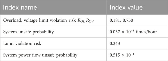
Table 1. Calculated weight values for each index.

4.2 Data-driven analysis

In XGBoost, there are three methods for calculating variable importance: using the frequency of variable splitting in trees as a measure of importance, using the average gain after variable splitting as a measure of profit, and using the coverage range of samples after variable splitting as a measure of coverage. In this section, the XGBRegressor function is used to train and learn from sample data. The number of iterations is set to 300, and other parameters are set, as shown in Table 2.

Table 2

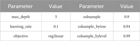
Table 2. Parameter setting.

The importance of variables in the model is analyzed. The analysis results are shown in Figure 5.

Figure 5

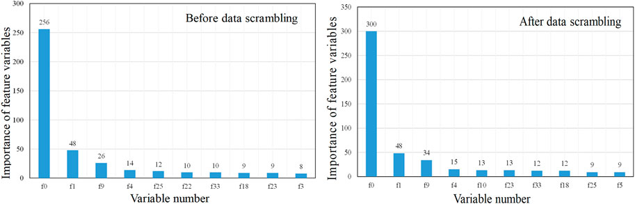
Figure 5. Before and after data scrambling importance analysis of feature variables based on XGBoost.

The specific SSA values and their accuracy rates for different operating scenarios of the system are shown in Figure 6 the average static security assessment values of prediction and actual are 1.470% and 1.472%.

Figure 6

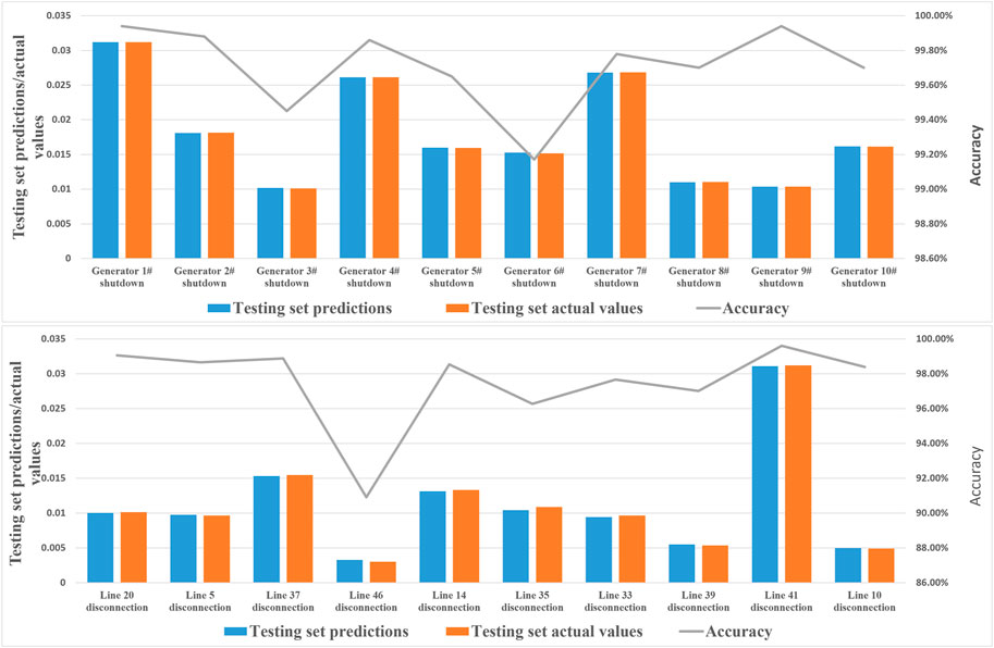
Figure 6. Static security assessment values and accuracy rates for different operating scenarios.

To provide a more intuitive analysis of the effectiveness of the strategies learned by the static assessment model based on the XGBoost algorithm, it will be compared to three methods: random forest regression, linear regression, and decision tree. Mean absolute error (MAE), R-squared score (R2_score), mean squared error (MSE), and root mean squared error (RMSE) are used as evaluation metrics. In all experiments, 80% of randomly sampled input data is used to build the model (training set), while 20% of the data is used for evaluation (testing set). The experimental results are shown in Table 3.

Table 3

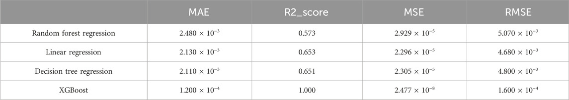
Table 3. Result comparison.

The experimental results indicate that the data-driven model used in this article has higher prediction accuracy than other comparative algorithms, demonstrating the better applicability of the XGBoost algorithm. The inference speed of the XGBoost algorithm is 7.58 × 10⁻⁶ s per item, showing a significant speed improvement compared to traditional evaluation methods.

5 Conclusion

This article outlines a static security assessment index system that accommodates stochastic variations, introduces a method based on stochastic load flow simulations, and develops a data-driven acceleration algorithm to enhance static security assessments in the face of stochastic variations.

First, based on simulation techniques, a calculation method for stochastic load flow is proposed, which can then provide the necessary indices for static security assessment considering uncertainties.

Second, by integrating the outcomes derived from stochastic load flow analyses, a comprehensive approach to static security assessments is adopted, focusing on two primary factors: the potential for branch overloading and the adherence to node voltage limits, evaluated specifically for each branch and node. The system indices are weighted considering both subjective and objective perspectives, and the safety assessment indices for new energy systems are ultimately obtained.

Third, for acceleration, the article utilizes data from various fault scenarios to create samples that are suitable for data-driven models, capturing the system’s stochastic load flow and voltage amplitude under both normal and fault conditions. An XGBoost-based data-driven model was developed using this dataset, specifically for safety assessment in new energy power systems. The XGBoost showed strong predictive accuracy in assessing the safety of these power systems in case studies.

The article effectively evaluates system safety under the influence of randomness, providing theoretical support and technical guidance for the stable operation of renewable power systems.

Data availability statement

The raw data supporting the conclusions of this article will be made available by the authors, without undue reservation.

Author contributions

YZ: writing–original draft, writing–review and editing. XT: writing–original draft, writing–review and editing. LZ: writing–original draft, writing–review and editing.

Funding

The author(s) declare that financial support was received for the research, authorship, and/or publication of this article. This work is sponsored by the Science and Technology Project of the State Grid Shandong Electric Power Company, Grant/Award Number: 520625210007.

Conflict of interest

Authors YZ, XT, and LZ were employed by the Economic & Technology Research Institute of the State Grid Shandong Electric Power Company.

The authors declare that this study received funding from State Grid Shandong Electric Power Company. The funder had the following involvement in the study: the collection of data work in this paper.

Publisher’s note

All claims expressed in this article are solely those of the authors and do not necessarily represent those of their affiliated organizations, or those of the publisher, the editors and the reviewers. Any product that may be evaluated in this article, or claim that may be made by its manufacturer, is not guaranteed or endorsed by the publisher.

References

Afrasiabi, S., Afrasiabi, M., Parang, B., and Mohammadi, M. (2019). Integration of accelerated deep neural network into power transformer differential protection. IEEE Trans. Industrial Inf. 16, 865–876. doi:10.1109/tii.2019.2929744

CrossRef Full Text | Google Scholar

Al-Sumaiti, A. S., Ahmed, M. H., Rivera, S., El Moursi, M. S., Salama, M. M., and Alsumaiti, T. (2019). Stochastic PV model for power system planning applications. IET Renew. Power Gener. 13, 3168–3179. doi:10.1049/iet-rpg.2019.0345

CrossRef Full Text | Google Scholar

Binder, K., Heermann, D. W., and Binder, K. (1992). Monte Carlo simulation in statistical physics. Springer.

Google Scholar

Čepin, M. (2011). Assessment of power system reliability: methods and applications. Springer Science & Business Media.

Google Scholar

Chatzimouratidis, A. I., and Pilavachi, P. A. (2007). Objective and subjective evaluation of power plants and their non-radioactive emissions using the analytic hierarchy process. Energy policy 35, 4027–4038. doi:10.1016/j.enpol.2007.02.003

CrossRef Full Text | Google Scholar

Chen, S., Chen, Q., Xia, Q., Zhong, H., and Kang, C. (2015). N 1 security assessment approach based on the steady-state security distance, 9. London, United Kingdom: Generation Transmission & Distribution Iet, 2419–2426.

CrossRef Full Text | Google Scholar

Chen, T., and Guestrin, C. (2016). “Xgboost: a scalable tree boosting system,” in Proceedings of the 22nd acm sigkdd international conference on knowledge discovery and data mining, 785–794.

Google Scholar

Conti, S., and Raiti, S. (2007). Probabilistic load flow using Monte Carlo techniques for distribution networks with photovoltaic generators. Sol. Energy 81, 1473–1481. doi:10.1016/j.solener.2007.02.007

CrossRef Full Text | Google Scholar

Das, D. (2007). Electrical power systems. New Age International.

Google Scholar

De La Ree, J., Liu, Y., Mili, L., Phadke, A. G., and Dasilva, L. (2005). Catastrophic failures in power systems: causes, analyses, and countermeasures. Proc. IEEE 93, 956–964. doi:10.1109/jproc.2005.847246

CrossRef Full Text | Google Scholar

Ghiasi, M. (2018). A detailed study for load flow analysis in distributed power system. Int. J. Industrial Electron. Control Optim. 1, 153–160. doi:10.22111/IECO.2018.24423.1027

CrossRef Full Text | Google Scholar

Graham, C., and Talay, D. (2013). Stochastic simulation and Monte Carlo methods: mathematical foundations of stochastic simulation. Springer Science and Business Media.

Google Scholar

Han, J., Miao, S., Li, Y., Yang, W., and Yin, H. (2021). Fault diagnosis of power systems using visualized similarity images and improved convolution neural networks. IEEE Syst. J. 16, 185–196. doi:10.1109/jsyst.2021.3056536

CrossRef Full Text | Google Scholar

Hu, Z., and Wang, X. (2007). Stochastic optimal load flow method considering load probability distribution. Automation Electr. Power Syst. (16), 14–18+44. doi:10.3321/j.issn:1000-1026.2007.16.003

CrossRef Full Text | Google Scholar

Ibrahim, M. A. (2011). Disturbance analysis for power systems. John Wiley & Sons.

Google Scholar

Jing, W. (2014). Functional modeling methodology of complex system and its application in safety assessment. Beijing: China University of Petroleum.

Google Scholar

Kalyani, S., and Swarup, K. S. (2010). Classification and assessment of power system security using multiclass SVM. IEEE Trans. Syst. Man, Cybern. Part C Appl. Rev. 41, 753–758. doi:10.1109/tsmcc.2010.2091630

CrossRef Full Text | Google Scholar

Kiruthika, M., and Bindu, S. (2020). Classification of electrical power system conditions with convolutional neural networks. Eng. Technol. Appl. Sci. Res. 10, 5759–5768. doi:10.48084/etasr.3512

CrossRef Full Text | Google Scholar

Meegahapola, L. G., Bu, S., Wadduwage, D. P., Chung, C. Y., and Yu, X. (2020). Review on oscillatory stability in power grids with renewable energy sources: monitoring, analysis, and control using synchrophasor technology. IEEE Trans. Industrial Electron. 68, 519–531. doi:10.1109/tie.2020.2965455

CrossRef Full Text | Google Scholar

Mohammadi, M., Gharehpetian, G., and Niknam, T. (2010). On-line small-signal stability assessment of power systems using ball vector machines. Electr. Power Components Syst. 38, 1427–1445. doi:10.1080/15325001003735150

CrossRef Full Text | Google Scholar

Morales, J. M., and Perez-Ruiz, J. (2007). Point estimate schemes to solve the probabilistic power flow. IEEE Trans. power Syst. 22, 1594–1601. doi:10.1109/tpwrs.2007.907515

CrossRef Full Text | Google Scholar

Prabhakar, P., Krishan, R., and Pullaguram, D. R. (2022). “Static security assessment of large power systems under n-1-1 contingency,” in 2022 22nd national power systems conference (NPSC). IEEE, 35–40.

CrossRef Full Text | Google Scholar

Qian, T., Shi, F., Wang, K., Yang, S., Geng, J., Li, Y., et al. (2022). N-1 static security assessment method for power grids with high penetration rate of renewable energy generation. Electr. Power Syst. Res. 211, 108200. doi:10.1016/j.epsr.2022.108200

CrossRef Full Text | Google Scholar

Rao, K. D., Gopika, V., Rao, V. S., Kushwaha, H., Verma, A. K., and Srividya, A. (2009). Dynamic fault tree analysis using Monte Carlo simulation in probabilistic safety assessment. Reliab. Eng. Syst. Saf. 94, 872–883. doi:10.1016/j.ress.2008.09.007

CrossRef Full Text | Google Scholar

Schavemaker, P., and Van Der Sluis, L. (2017). Electrical power system essentials. John Wiley & Sons.

Google Scholar

Shirasaki, K., and Uchida, N. (2010). Fast computation and stable convergence technique for unbalanced load flow calculation in the large scale system. IEEJ Trans. Power Energy 128, 1329–1334. doi:10.1541/ieejpes.128.1329

CrossRef Full Text | Google Scholar

Su, C.-L. (2005). Probabilistic load-flow computation using point estimate method. IEEE Trans. Power Syst. 20, 1843–1851. doi:10.1109/tpwrs.2005.857921

CrossRef Full Text | Google Scholar

Thomopoulos, N. T. (2012). Essentials of Monte Carlo simulation: statistical methods for building simulation models. Springer Science & Business Media.

Google Scholar

Tuinema, B. W., Tuinema, B. W., Rueda Torres, J. L., Stefanov, A. I., Gonzalez-Longatt, F. M., and Van Der Meijden, M. A. (2020). “Probabilistic power flow analysis,” in Probabilistic reliability analysis of power systems: a student’s introduction, 179–208.

CrossRef Full Text | Google Scholar

Wang, X.-F., Song, Y., and Irving, M. (2008). Load flow analysis. Mod. power Syst. Anal., 71–128.

Google Scholar

Wang, L., Lin, X., Howell, F., and Morison, K. (2016). Dynamic security assessment. Smart grid handbook, 1–24.

CrossRef Full Text | Google Scholar

Wu, X. Z. (2015). Assessing the correlated performance functions of an engineering system via probabilistic analysis. Struct. Saf. 2015, 10–19. doi:10.1016/j.strusafe.2014.07.004

CrossRef Full Text | Google Scholar