Small-disturbance stability analysis and control-parameter optimization of grid-connected virtual synchronous generator

The virtual synchronous generator (VSG) has been widely used to improve the system inertia and damping in the renewable energy generation system. However, the in-depth understanding of VSG’s stability under disturbances on different control parameters is lacked. In order to solve the problem, the small-signal model of single-VSG is established at first. The influences of key control parameters on the stability of system are analyzed by using the eigenvalue analysis method in detail. On this basis, a novel optimization strategy for control parameters is proposed based on the Particle Swarm Optimization (PSO) algorithm. The control parameters are optimized to realize excellent damping and stability of VSG system. Finally, the simulation and experimental results verify the effectiveness of stability analysis and parameter optimization strategy.

1 Introduction

With the development of new energy sources, many new energy units are connected to the grid by traditional inverters (Du et al., 2020; Zhang et al., 2021). However, traditional grid-connected inverters cannot participate in grid regulation. This will result in a decrease in the overall inertia and damping of the power system, which brings serious challenges to the stable operation of system (Pattabiraman et al., 2018). In order to ensure the stable operation of the power system under the high penetration rate of new energy, related literature have proposed the concept of Virtual Synchronous Generator (VSG) by referring to the operating characteristics and principles of the traditional synchronous generator, and carried out extensive researches on the control strategy, stability analysis, and parallel connection of multiple machines (Xiong et al., 2016; Choopani et al., 2020).

In the study of grid-connected stability of VSG, a VSG and an SG were connected in (Baruwa and Fazeli, 2021) for analyzing the low-frequency oscillation phenomenon after the VSG replaces the SG, as well as the characteristics and main modes of low-frequency oscillations. Literature (Lu et al., 2022) analyzes the impacts of VSG parameter changes by eigenvalue analysis method. But it does not give any advice on how the parameters should be designed.

The parameters design of the VSG has been discussed (Du et al., 2013), Due to the equivalence of the VSG and droop control, the parameters design methods of droop control also provide the design guidance for the VSG(Coelho et al., 1999; Guerrero et al., 2007; Guerrero et al., 2004). The root-locus design method was used in literature (Du et al., 2013), but it is just the design of a separate power loop, thus the designed parameters may not be good enough and they are needed to be further adjusted to obtain the optimized results. Literature (D’Arco and Suul, 2014) derives the closed-loop characteristic equations of the power loop with droop control. However, due to the coupling effect between the active and reactive power loops the parameter design of the two loops is very difficult and the control parameters are partially tuned by trial and error. Similarly, Literature (Wu et al., 2016) has developed a small-signal model of the VSG power loop and proposed a step-by-step parameter design methodology that takes into account the stability and dynamic performance of the VSG. However, there is no detailed study of VSG parameter variations on its stability. Literature (Wu et al., 2019; Xu et al., 2021) provide impedance modeling and stability analysis for virtual synchronous control of permanent magnet wind turbines. However, the impedance characteristic curve can only reflect the external characteristics of the system, and the relationship with each internal controller or parameter is not clear. Literature (D’Arco et al., 2015; D’Arco et al., 2013) indicate that there are interactions between the cascade control loops contained in the VSG system, and the VSG system dynamics equations are relatively complex. For these reasons, it can be seen that the current literature on the parameter design method for VSGs is only designed independently for each control loop and does not consider the coupling effect of the overall parameters. Classical tuning methods to this scheme are difficult to use.

Therefore, small-signal modeling of a stand-alone grid-connected system is carried out in this paper. Meanwhile, the effect of each control loop on the small-signal stability of the system is comprehensively considered in this paper. A detailed analysis of the active power loop control parameters, virtual impedance, and voltage loop of a single-unit grid-connected system is presented in this paper. Based on the above analysis, this paper proposes a PSO-based global control parameter optimization algorithm for multiple operating points. The optimized control parameters are used to provide better dynamic performance and stability at different grid strengths.

The rest of this paper is organized as follows: Section 2 provides a brief description of VSG control strategy and small-signal model of single-VSG grid-connected System. In Section 3, Eigenvalue analysis based on the small signal model of the system reveals that power loops, virtual impedances, and voltage loops have a large impact on system stability. Therefore, the influences of control parameters of active power loop, virtual impedance and voltage loop on the stability of the system are analyzed in detail. Section 4 presents a coordinated optimization strategy of control parameters based on PSO. In Section 5, the above analysis is verified by PSCAD simulation, and then Section 6 presents the experimental results obtained with coordinated optimization method and stability analysis. Finally, conclusions are presented in Section 7.

2 Small-signal model of Single-VSG grid-connected system

2.1 Control strategy

The control block diagram of VSG is shown in Figure 1. The control strategy of VSG can be divided into four parts. The first part is the power loop controller, which is composed of active-power-frequency control and reactive-power-voltage control. Active-power-frequency control can simulate the inertia and damping of synchronous generators. Reactive-power-voltage control can simulate the primary regulation of synchronous generators. The second part is the virtual impedance control, which is used to reshape the output impedance of VSG. The third part is the voltage-current double closed-loop controller, which consists of outer voltage and inner current closed-loop modules. The fourth part contains the dq/abc transformation as well as sinusoidal pulse width modulation.

Figure 1

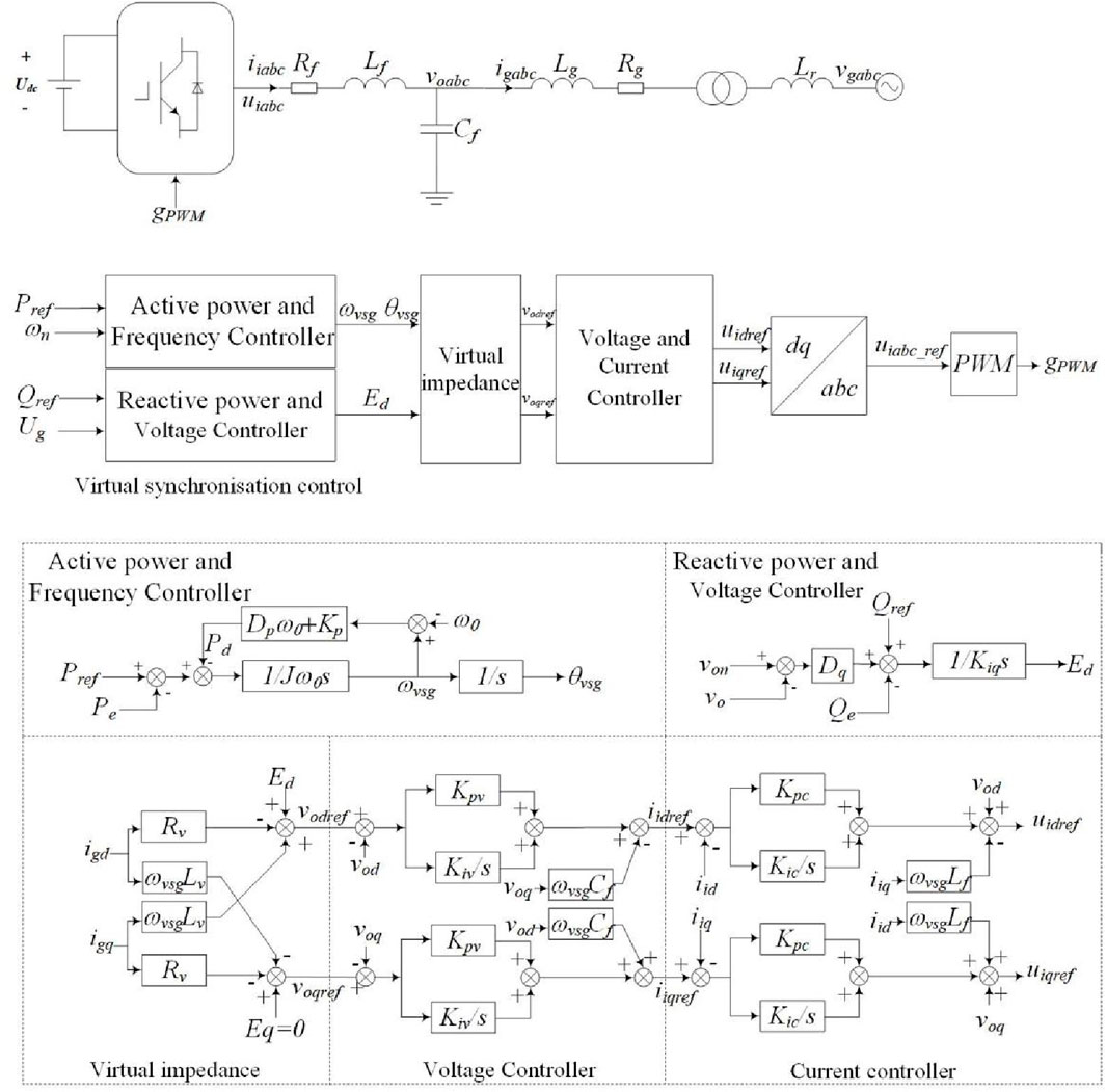
Figure 1. Topology diagram of VSG.

In Figure 1, u_dc is the ideal DC voltage on the DC side, R_f is filter resistance, L_f is filter inductance, and C_f is filter capacitance. R_g and L_g are the resistance and inductance of the connecting line. v_iabc are the output voltage of the inverter. v_oabc are the voltage across filter capacitance. i_iabc are the output currents of the inverter. i_gabc are the currents of the line inductance. u_gabc are the AC power grid voltages. P_ref is the active power reference, and Q_ref is the reactive power reference. ω_vsg is the virtual angular frequency. ω₀ is the rated angular frequency of VSG. K_d is the active frequency regulation coefficient of the governor. P_e is the measured electrical power. J is the virtual inertia of VSG, D_p is the virtual damping coefficient, and θ_vsg is the phase angle that is the integral of the virtual angular frequency. K_q is the regulation coefficient of reactive-power-voltage. v_oref is voltage amplitude reference. v_o is the amplitude of capacitor voltage. The variables with subscripts d or q indicate variables in dq coordinates.

2.2 Modelling

The detailed modeling process of VSG has been described in Literature (Pogaku et al., 2007; Li et al., 2023). Therefore, this paper will not repeat the details. A non-linear model of the single-VSG grid-connected system can be established by Eq. (1).

$\left\{\begin{array}{l}J{\omega }_0\frac{d{\omega }_{vsg}}{dt}=P_{ref}-P_e-\left(D_p{\omega }_0+K_p\right)\left({\omega }_{vsg}-{\omega }_0\right)\\ K_{iq}\frac{d{E}_d}{dt}=Q_{set}+K_q\left(v_{on}-v_o\right)-Q_e\\ v_{odref}+j{v}_{oqref}=E_d-i_{gd}{R}_v+i_{gq}{w}_{vsg}{L}_v+j\left(-i_{gq}{R}_v-i_{gd}{w}_{vsg}{L}_v\right)\\ i_{idref}+i_{iqref}=K_{pv}\left(v_{odref}-v_{od}\right)+K_{iv}{x}_{ud}-v_{oq}{w}_{vsg}{C}_f+j\left(K_{pv}\left(v_{oqref}-v_{oq}\right)+K_{iv}{x}_{uq}+v_{od}{w}_{vsg}{C}_f\right)\\ \frac{d{x}_{ud}}{dt}+j\frac{d{x}_{uq}}{dt}=v_{odref}-v_{od}+j\left(v_{oqref}-v_{oq}\right)\\ u_{idref}+j{u}_{iqref}=v_{od}+K_{pc}\left(i_{idref}-i_{id}\right)+K_{ic}{x}_{id}-i_{iq}{w}_{vsg}{L}_f+j\left(v_{oq}+K_{pc}\left(i_{iqref}-i_{iq}\right)+K_{ic}{x}_{iq}+i_{id}{w}_{vsg}{L}_f\right)\\ \frac{d{x}_{id}}{dt}+j\frac{d{x}_{iq}}{dt}=i_{idref}-i_{id}+j\left(i_{iqref}-i_{iq}\right)\\ \frac{d{i}_{id}}{dt}+j\frac{d{i}_{iq}}{dt}=-\frac{R_f}{L_f}{i}_{id}+w_{vsg}{i}_{iq}+\frac{1}{L_f}{v}_{id}-\frac{1}{L_f}{v}_{od}+j\left(-\frac{R_f}{L_f}{i}_{iq}-w_{vsg}{i}_{iq}+\frac{1}{L_f}{v}_{iq}-\frac{1}{L_f}{v}_{oq}\right)\\ \frac{d{v}_{od}}{dt}+j\frac{d{v}_{oq}}{dt}=w_{vsg}{v}_{oq}+\frac{1}{C_f}{i}_{id}-\frac{1}{C_f}{i}_{gd}+j\left(-w_{vsg}{v}_{od}+\frac{1}{C_f}{i}_{id}-\frac{1}{C_f}{i}_{gd}\right)\\ \frac{d{i}_{gd}}{dt}+j\frac{d{i}_{gq}}{dt}=-\frac{R_g}{L_g}{i}_{gd}+w_{vsg}{i}_{gq}+\frac{1}{L_g}{v}_{od}-\frac{1}{L_g}{v}_{bd}+j\left(-\frac{R_g}{L_g}{i}_{gq}-w_{vsg}{i}_{gd}+\frac{1}{L_g}{v}_{oq}-\frac{1}{L_g}{v}_{bq}\right)\\ v_{bd}+j{v}_{bq}=E_{gd}\cos \left(\delta \right)+j{E}_{gd}\sin \left(\delta \right)\\ \frac{d\delta }{dt}=w_g-w_{vsg}\end{array}\right.(1)$

The above nonlinear equations can be simplified and linearized at the steady state point. Consequently, the small-signal model of single-VSG grid-connected system can be obtained as Eq. (2)

$\frac{d\Delta x_{sys}}{dt}=\mathbf{A}\Delta x_{sys}+\mathbf{B}\Delta u(2)$

In Eq. (2), Δx_sys is the state variable vector of the system, Δu is the input variable vector of the system, and the elements of matrices A and B are related to the steady state point. Matrices A and B are given in Supplementary Materia S1–S3.

3 Stability analysis of Single-VSG grid-connected system

3.1 Oscillation mode analysis of Single-VSG system

According to the small-signal model described by Eq. (2), all eigenvalues of the system matrix A are obtained based on the system parameters in Table 1. The oscillation modes of system and the effect of parameter variations on the stability can be obtained by analyzing the eigenvalue distribution.

Table 1

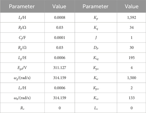
Table 1. Parameters of single-VSG system.

The system eigenvalues are shown in Table 2. It can be concluded that the system has thirteen eigenvalues, corresponding to seven oscillation modes. There are 6 pairs of conjugate complex eigenvalues and 1 real eigenvalue. They correspond to 7 oscillation modes. The system is stable on condition that the eigenvalues of the system are in the left half plane of the complex plane. By using the participation factor analysis, it can be obtained that λ_1∼4 are mainly associated with the state variables i_id, i_iq, v_od, and v_oq generated by the LC filters. However, the distances between the eigenvalues λ_1∼4 and the imaginary axis are much greater than the distances between other eigenvalues and the imaginary axis. As a result, λ_1∼4 have little influence on the system stability and can be ignored. λ_5∼6 are mainly associated with the state variables i_gd and i_gq. λ_7∼8 are mainly associated with the state variables x_id and x_iq generated by the current loop control. λ_9∼10 and λ_12∼13 are mainly associated with the state variables x_ud and x_uq generated by the voltage loop control as well as the state variables ω_vsg and δ generated by the active-power-frequency control. The influences of various controller parameters on system stability are presented in the following parts of this section.

Table 2

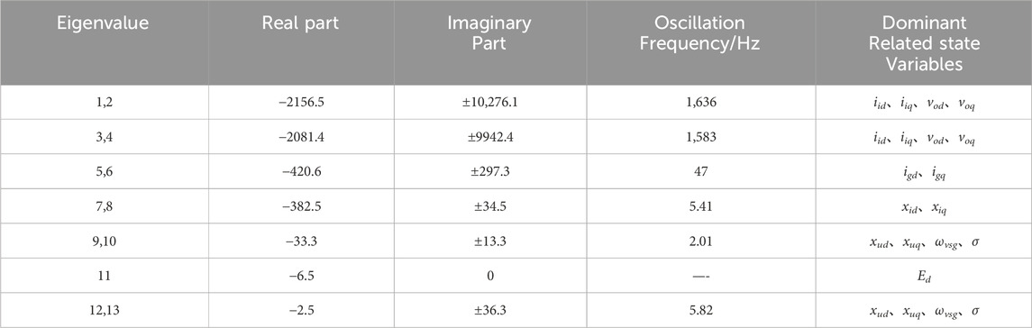
Table 2. Eigenvalues of single-VSG system.

3.2 Controller parameters of active-power-frequency loop

The control parameters of active-power-frequency loop include the virtual inertia J and the virtual damping coefficient D_p. The eigenvalue trajectories with the changes of parameter are shown in Figure 2.

Figure 2

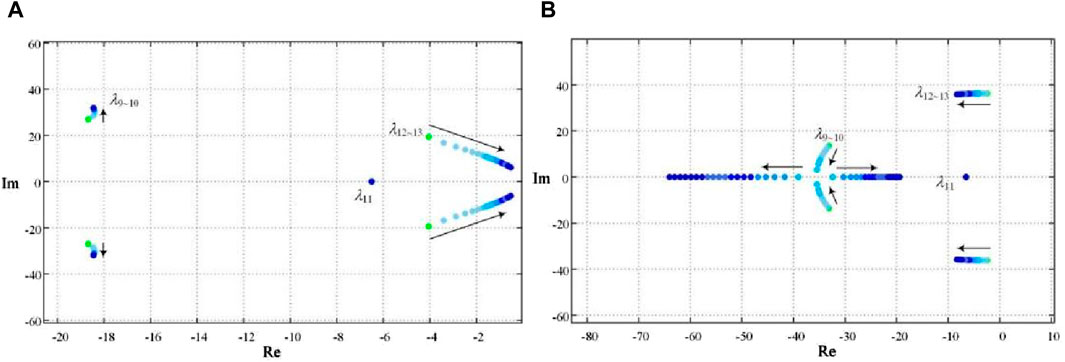
Figure 2. The eigenvalue trajectories under different control parameters of active-power-frequency loop. (A) Eigenvalue trajectories of the system under different inertias. (B) Eigenvalue trajectories of the system under different damping coefficients.

When the virtual inertia J changes from 4 to 40 and other parameters remain unchanged, the eigenvalue trajectories are shown in Figure 2A. With the increase in virtual inertia, the eigenvalues λ_1–10 have slight changes. However, the eigenvalues λ_12–13 move towards the imaginary axis rapidly. It is evident that the damping ratio of the corresponding oscillation mode decreases rapidly while the oscillation frequency decreases slightly. As a result, the system stability is deteriorated.

When the virtual damping coefficient D_p changes from 30 to 60 and other parameters remain unchanged, the eigenvalue trajectories are shown in Figure 2B. With the increase in virtual damping coefficient, the eigenvalues λ_1–8 and λ₁₀ have slight changes. The eigenvalues λ_12–13 move to the left of the complex plane and the movement speed away from the imaginary axis is much higher than that away from the real axis. It can be concluded that the damping ratio of the corresponding oscillation mode increases, the overshoot gradually decreases, the oscillation frequency increases slightly, and the system stability is improved. However, the eigenvalues λ_9–10 firstly move away from the right half plane and towards the real axis; then moves to the right half plane along the real axis. Therefore, the virtual damping coefficient D_p should not be too large, otherwise the system stability will be deteriorated.

3.3 Virtual impedance parameters

The virtual impedance parameters include the virtual resistor R_v and the virtual inductor L_v. The eigenvalue trajectories with the parameter changes are shown in Figure 3.

Figure 3

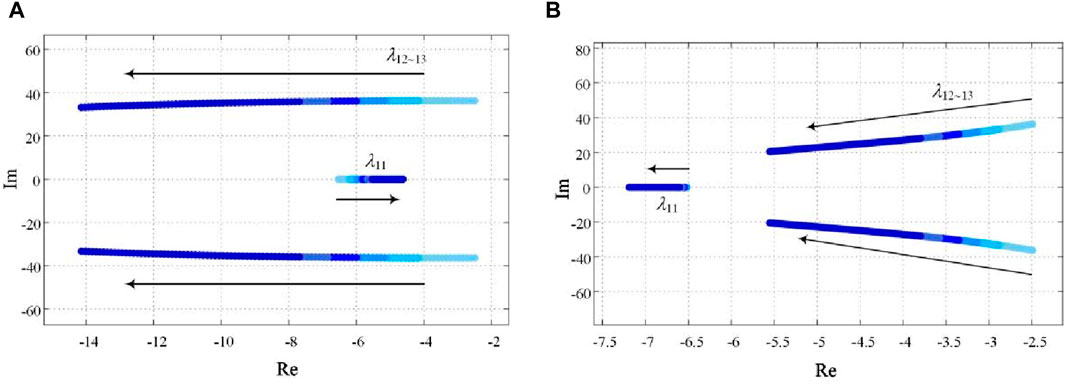
Figure 3. The eigenvalue trajectories under different virtual impedance parameters. (A) Eigenvalue trajectories of the system under different virtual inductor. (B) Eigenvalue trajectories of the system under different virtual resistor.

When the virtual inductor L_v changes from 0 to 0.0005, other parameters remain unchanged, and the eigenvalue trajectories is shown in Figure 3A. With the increase in virtual inductor L_v, the eigenvalues λ_1–10 has little changed. However, the eigenvalues λ_12–13 move rapidly away from the imaginary axis, the damping ratios of the corresponding oscillation attenuation mode increase rapidly, the oscillation frequency decreases slightly, and the system stability improved. Meanwhile, the eigenvalues λ₁₁ gradually approaches the imaginary axis, and the system will be slightly worse for stability.

When the virtual resistor R_v changes from 0 to 0.3, other parameters remain unchanged, and the eigenvalue trajectories is shown in Figure 3B. With the increase in virtual resistor R_v, the eigenvalues λ_1–10 has little changed. However, the eigenvalues λ_12–13 move rapidly away from the imaginary axis, the damping ratios of the corresponding oscillation attenuation mode increase rapidly, the oscillation frequency decreases slightly, and the system stability improved. Unlike the trajectory of the eigenvalues when the virtual inductor changes, the eigenvalues λ₁₁ also moves away from the imaginary axis, and the stability of the system will be further improved.

3.4 Control parameters of voltage loop

The voltage loop controller parameters include proportionality coefficient K_pv and the integrity coefficient K_iv. The eigenvalue trajectories with the parameter changes are shown in Figure 4.

Figure 4

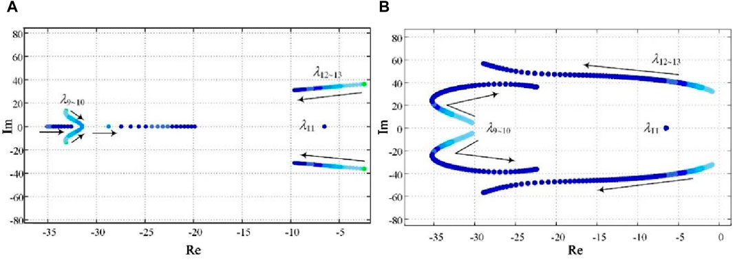
Figure 4. The eigenvalue trajectories under different voltage loop controller parameters. (A) Eigenvalue trajectories of the system under different proportionality coefficient. (B) Eigenvalue trajectories of the system under different integrity coefficient.

When the proportionality coefficient K_pv changes from 2 to 20, other parameters remain unchanged, and the eigenvalue trajectories is shown in Figure 4A. With the increase in proportionality coefficient K_pv, the eigenvalues λ_12–13 move rapidly away from the imaginary axis, the damping ratios of the corresponding oscillation attenuation mode increase rapidly, the oscillation frequency decreases slightly, and the system stability improved. However, the eigenvalues λ_9-10 gradually approaches the right half plane after changing to the real axis from a pair of conjugate complex roots, and the system will be slightly worse for stability. Therefore, the proportionality coefficient should not be too large.

When the integrity coefficient K_iv changes from 100 to 400, other parameters remain unchanged, and the eigenvalue trajectories is shown in Figure 4B. With the increase in integrity coefficient K_iv, the eigenvalues λ_12–13 also move rapidly away from the imaginary axis, the damping ratios of the corresponding oscillation attenuation mode increase rapidly, the oscillation frequency decreases slightly, and the system stability improved. However, the eigenvalues λ_9-10 first moves away from the imaginary axis and then gradually moves closer to the imaginary axis. Therefore, the integrity coefficient also should not be too large.

3.5 Different short circuit ratios

The eigenvalue trajectories with different short circuit ratios are shown in Figure 5.

Figure 5

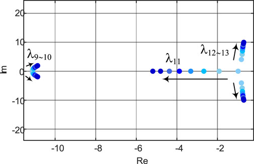
Figure 5. The eigenvalue trajectories under different short circuit ratio.

When the short circuit ratio changes from 1 to 8 and other parameters remain unchanged, the eigenvalue trajectories are shown in Figure 5. With the increase in short circuit ratio, the eigenvalues λ_12–13 move towards the right-half plane rapidly. It is evident that the damping ratio of the corresponding oscillation mode decreases rapidly while the oscillation frequency increase slightly. Although the eigenvalue λ₁₁ is moving to the left half plane, the eigenvalue λ_12–13 is closer to the right half plane. As the short-circuit ratio is increasing, the system becomes less stable.

4 Optimization strategy for control parameters based on PSO

4.1 PSO algorithm

The basic idea of the PSO algorithm is to assume that there are N1 particles in the D-dimensional space, and the particles update their velocities and positions according to Eq. (3).

$\left\{\begin{array}{c}{v}_{ij}^{k+1}=w{v}_{ij}^k+r_1{a}_1\left(p_{ij}-x_{ij}^k\right)+r_2{a}_2\left(p_{kj}-x_{ij}^k\right)\\ x_{ij}^{k+1}=x_{ij}^k+v_{ij}^k\end{array}\right.(3)$

In Eq. (3), w is the inertia weight; r1 and r2 are uniform random numbers in the range of [0, 1]; a1 and a2 are the learning factors; v^k_ij and x^k_ij are the velocity and position of particle i in the kth iteration, respectively, and both of them are restricted to be movable; p_ij is the optimal position experienced by the ith particle; and p_gj is the optimal position experienced by all particles of the particle swarm.

4.2 The objective function

It can be known from the above: the stability performance of the system depends on the distribution of the eigenvalues, which depends on the design of the controller parameters. Therefore, the optimization objectives designed in this paper are as follows:

(1) All eigenvalues as far away from the right half plane as possible.

(2) The damping ratio of each oscillation mode should be as large as possible to minimize the number of oscillation cycles during the transient process.

According to the optimization objective, the objective function of the system under a single operating point is defined as Eq. (4).

$\begin{array}{l}\min E_j={\displaystyle \sum _{i=1}^N}{w}_{i}f\left({\lambda }_i\right)+{\displaystyle \sum _{i=1}^N}{k}_{i}h\left({\lambda }_i\right)\\ \left\{\begin{array}{l}f\left({\lambda }_i\right)=\left\{\begin{array}{cc}0& \text{Re}\left({\lambda }_i\right)\le \sigma \\ \text{Re}\left({\lambda }_i\right)-\sigma & \text{Re}\left({\lambda }_i\right)>\sigma \\ \inf & \text{Re}\left({\lambda }_i\right)\ge 0\end{array}\right.\\ h\left({\lambda }_i\right)=\left\{\begin{array}{cc}0& \frac{\left|\text{Re}\left({\lambda }_i\right)\right|}{\left|{\lambda }_i\right|}\ge \xi ,\text{Re}\left({\lambda }_i\right)<0\\ \xi -\frac{\left|\text{Re}\left({\lambda }_i\right)\right|}{\left|{\lambda }_i\right|}& \frac{\left|\text{Re}\left({\lambda }_i\right)\right|}{\left|{\lambda }_i\right|}<\xi ,\text{Re}\left({\lambda }_i\right)<0\\ \inf & \text{Re}\left({\lambda }_i\right)\ge 0\end{array}\right.\end{array}\right.\end{array}(4)$

In Eq. (4), N is the number of eigenvalues. Re (λ_i) is the real part of the eigenvalue λ_i. | λ_i | is the value of the modulus of the eigenvalue λ_i. ξ is the desired damping ratio. σ is the desired real part value. w_i is the weight of f (λ_i). k_i is the weight of h (λ_i). In this paper, we take σ = −15, ξ = 0.707 and w_i and k_i are taken as shown in Eq. (5).

$w_i=\left\{\begin{array}{cc}0.01& \text{Re}\left({\lambda }_i\right)<\delta \\ 0.1& \delta <\text{Re}\left({\lambda }_i\right)<0.5\delta \\ 0.8& 0.5\delta <\text{Re}\left({\lambda }_i\right)<0\\ 1& \text{Re}\left({\lambda }_i\right)>0\end{array}\right.,k_i=\left\{\begin{array}{cc}0.01& \frac{\left|\text{Re}\left({\lambda }_i\right)\right|}{\left|{\lambda }_i\right|}>\xi \\ 10& 0.5\xi <\frac{\left|\text{Re}\left({\lambda }_i\right)\right|}{\left|{\lambda }_i\right|}<\xi \\ 30& \frac{\left|\text{Re}\left({\lambda }_i\right)\right|}{\left|{\lambda }_i\right|}<0.5\xi \end{array}\right.(5)$

Considering different grid strengths as well as different output powers in practice, the VSG can be linearized at different steady state operating points, and then the eigenvalues corresponding to each operating point can be solved separately. Therefore, in order to consider the effectiveness of the control parameters under multiple operating points, the objective function is changed to Eq. (6) based on a single operating point.

$\min E={\displaystyle \sum _{j=1}^M}{p}_j{E}_j(6)$

where p_j is the probability of the jth operating point, E_j is the optimization objective function at the jth operating point. In this way, the control parameters can be globally optimized for multiple operating conditions.

4.3 Optimization process

In the PSO algorithm, the objective function represents the fitness value of the particle, the controller parameter represents the position, the change value of the controller parameter represents the speed, the individual extreme value represents the optimal fitness value of each particle, the global extreme value represents the optimal fitness value searched by all the particles, and the position corresponding to the particle with the global extreme value is the optimal control parameter value. The algorithm flow is shown in Figure 6. Firstly, the particle velocity and particle position are initialized. The particle position is the main control parameter of the VSG and is represented by the vector [J D_p L_v R_v K_pv K_iv K_pc K_ic]. Secondly, the above control parameters are brought into the system eigenmatrix to obtain the system eigenvalues. The system eigenvalues are brought into the objective function to get the individual objective value for each particle. Updating the group historical optimum with the individual optimum based on the current individual objective function values. Update the particle positions by learning factor and inertia factor for several iterations. Finally, the particle positions corresponding to the population historical optimal values are the optimal control parameters of the VSG.

Figure 6

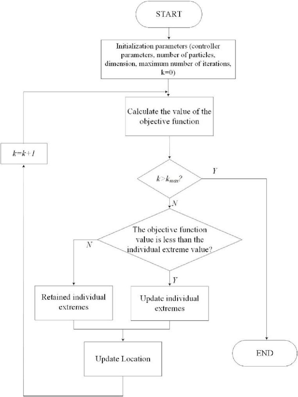
Figure 6. Flowchart of PSO algorithm.

4.4 Example analysis

The control parameters of the system are optimized by using a PSO-based multiple operating point optimization algorithm. And the control parameters of the system before and after optimization are shown in Table 3. The different work points are shown in Table 4 The population historical optimal fitness and the number of iterations is shown in Figure 7. As the number of iterations increases, the population historical optimal fitness rapidly converges. The distribution of eigenvalues before and after optimization is shown in Figure 8. The PSO algorithm was run several times. the population historical optimal fitness all converge to the optimal value relatively quickly, and the average number of convergence is about 65 times, which indicates that the optimization strategy of the PSO algorithm has a good convergence property, and the optimization results can be obtained within a limited number of iterations. The distribution of eigenvalues after optimization is further away from the imaginary axis than before optimization. However, the complex eigenvalue closest to the imaginary axis after optimization is close to the optimal damping ratio.

Table 3

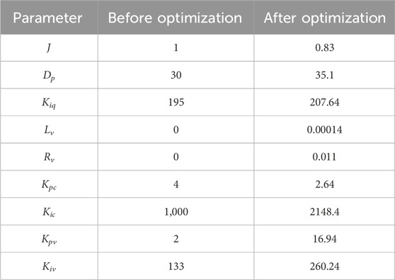
Table 3. Comparison of control parameters before and after optimization.

Table 4

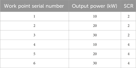
Table 4. Voltage source type D-PMSG with different operating conditions.

Figure 7

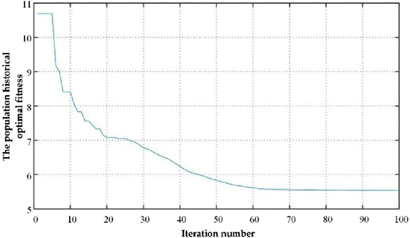
Figure 7. Population optimal fitness convergence curve.

Figure 8

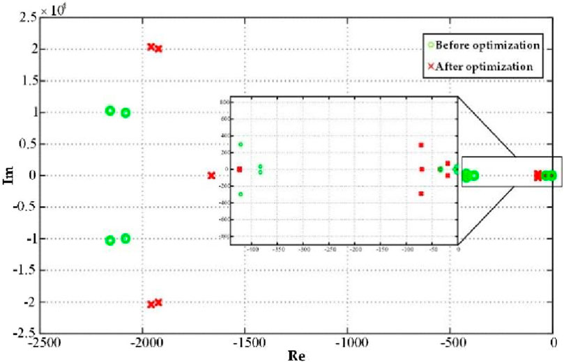
Figure 8. The distribution of eigenvalues before and after optimization.

5 Simulation verification

5.1 Small-signal model verification

To verify the correctness of the small-signal model derived above, the actual model was built in PSCAD according to the parameters in Table 1.

The change curves of each variable in the two models are shown in Figure 9 by comparing the change curves of each variable in the two models at 5 s for the active power reference value P_ref from a step of 5kW–10 kW. It can be observed that the dynamic process of the small-signal model basically overlaps with the PSCAD simulation model, which verifies the accuracy of the small-signal model established in this paper.

Figure 9

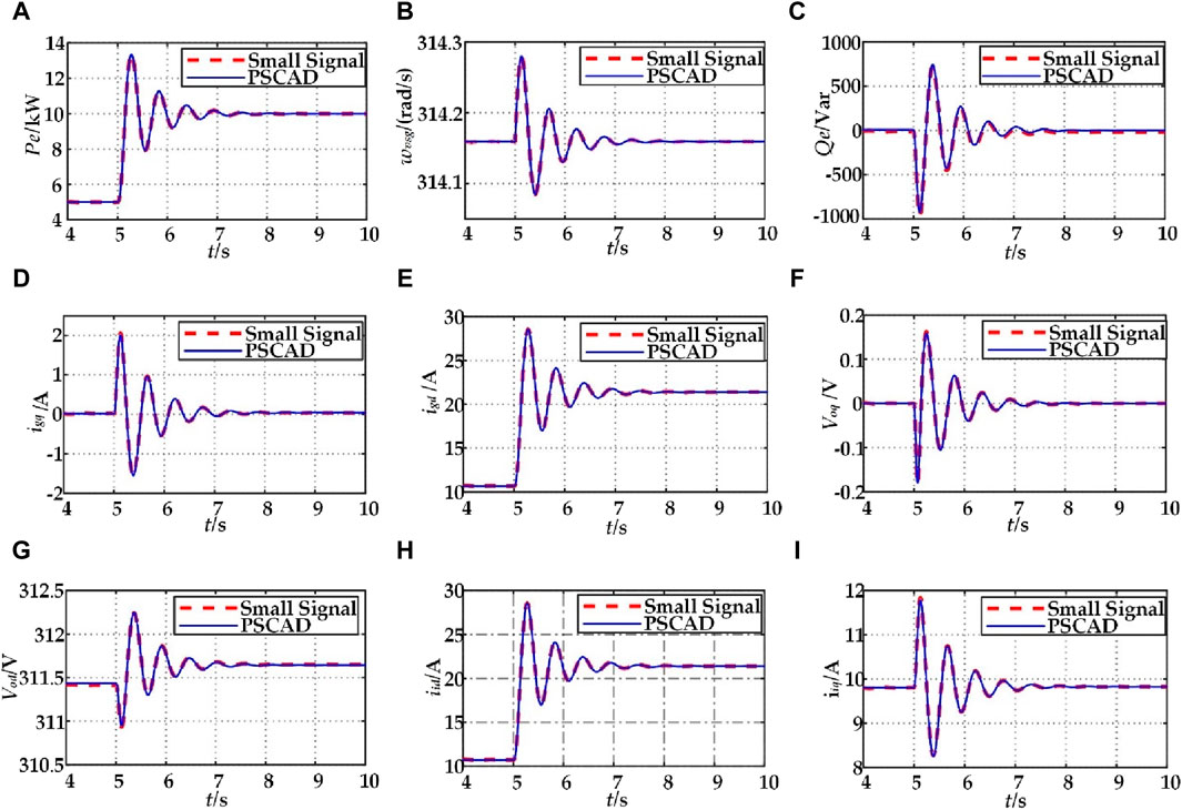
Figure 9. Comparison of simulation results between small signal model and PSCAD model: (A) Pe; (B) wvsg; (C) Qe; (D) igq; (E) igd; (F) voq; (G) vod; (H) iid; (I) iiq.

5.2 Stability analysis verification

To verify the correctness of the analysis of the above variable parameters on the change law of eigenvalue trajectories, a time domain simulation model of a VSG grid-connected system was built in PSCAD. With the same other parameters (as shown in Table 1), when the power is stepped, the response simulation waveforms under different virtual moments of inertia, virtual damping coefficients, virtual inductor, virtual resistor, voltage proportionality coefficients and voltage integration coefficients are shown in Figure 10A–E respectively.

Figure 10

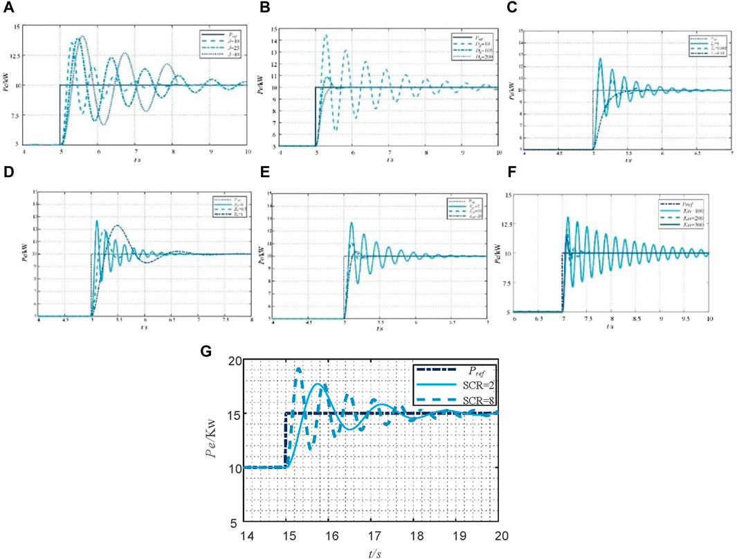
Figure 10. Simulation waveforms with parameters: (A) different virtual inertias; (B) different damping coefficients; (C) different virtual inductor; (D) different virtual resistors; (E) different proportionality coefficients; (F) different integrity coefficients; (G) different short circuit ratio.

As can be seen from Figures 10A,B, increasing the virtual inertia J or decreasing the virtual damping coefficient D_p will make the system unstable under a power stepping. Increasing the virtual inertia J influences the number of oscillations of active power and frequency under power stepping, increasing the regulation time of the system. Increasing the virtual damping coefficient D_p reduces the amplitude of oscillations of active power and frequency and shortens the time for the system to reach stability.

As can be seen from Figures 10C,D, decreasing the virtual inductor L_v or decreasing the virtual resistor R_v will make the system unstable under a power stepping. Decreasing the virtual inductor L_v influences the number of oscillations of active power and frequency under power stepping, increasing the regulation time of the system. Increasing the virtual resistors R_v reduces the amplitude of oscillations of active power and frequency and shortens the time for the system to reach stability.

As can be seen from Figures 10E,F, decreasing the voltage proportionality coefficients K_pv or decreasing the voltage integrity coefficients K_iv will make the system unstable under a power stepping. Decreasing the voltage proportionality coefficients K_pv influences the number of oscillations of active power and frequency under power stepping, increasing the regulation time of the system. Increasing the voltage integrity coefficients K_iv reduces the amplitude of oscillations of active power and frequency and shortens the time for the system to reach stability.

As can be seen from Figure 10G, increasing short circuit ratio will make the system unstable under a power stepping. Increasing short circuit ratio influences the number of oscillations of active power and frequency under power stepping. And it will increase the regulation time of the system.

5.3 Parameter optimization

To verify the validity of optimization strategy derived above, the actual model was built in PSCAD according to the parameters in Table 3. In order to simulate the large perturbation, the active power reference value Pref changes rapidly from 10Kw to 20Kw at t = 4 s, 20Kw to 30Kw at t = 6 s, 30Kw to 0Kw at t = 8 s, 0 to 30Kw at t = 12 s. The active power response curves at different short circuit ratios are shown in Figure 11A, B. It can be found that the stability of the system is improved even under large disturbances after using the optimization of multiple operating points. And the optimized system performs well at different short circuit ratios.

Figure 11

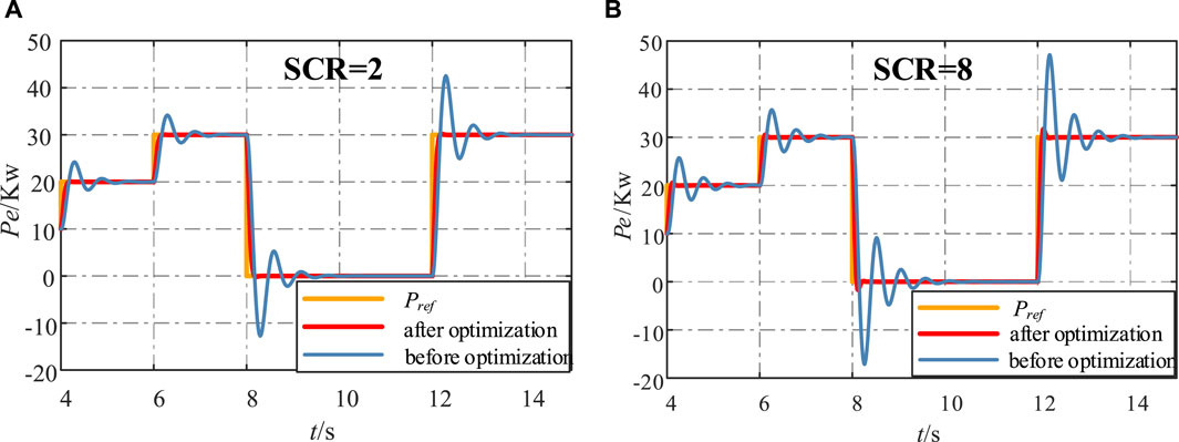
Figure 11. Simulation waveforms of active power before and after optimization for different short circuit ratios (SCR): (A) SCR = 2; (B) SCR = 8.

As can be seen from Figure 11A ∼ Figure 11B, Parameter optimization not only improves response speed, but also reduces oscillation amplitude. As a result, the system with optimized parameters has better response characteristics under different grid strengths and disturbances.

6 Experimental verification

To further verify the reliability and accuracy of the above theoretical analysis, a virtual synchronous machine model is built based on RT-LAB semi-physical simulation platform. And for the observation and verification, the parameters of the critically stabilized system are selected as shown in Table 5.

Table 5

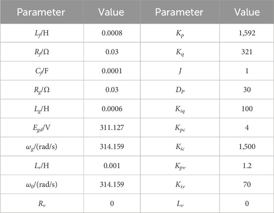
Table 5. VSG critically stabilized system parameters.

RT-LAB real-time simulation platform consists of an upper computer, a lower computer and a controller. The upper computer is an PC, the lower computer consists of OP5600 module produced by Opal-RT Canada, and the controller used TMS320F28379d DSP control chip. The detailed experimental platform is shown in Figure 12A. The experimental schema is shown in Figure 12B. The simulation model built in MATLAB/Simlink is put into the OP5600 real-time simulator for real-time operation, and the DSP controller receives the analog signals output from the OP5600 through the ADC module and executes the algorithmic procedures in the DSP to generate the corresponding PWM signals to be sent back to the main circuit through the digital port of the OP5600. The model realizes the complete control.

Figure 12

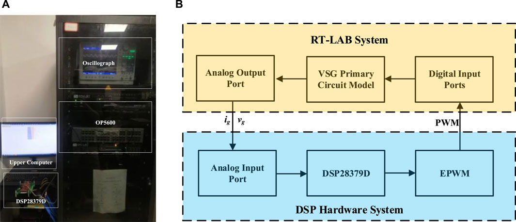
Figure 12. Experimental device and principle: (A) Experimental device; (B) The experimental schema.

Figure 13A illustrates the variation of the eigenvalues nearest to the imaginary axis when the virtual inertia coefficient J is changed. From the figure, it can be found that when J = 0.5, the eigenvalues are located in the left half plane and the system is in a stable state, corresponding to an oscillation frequency of 5.6 Hz for the eigenmode, and when J = 1, the eigenvalues are located in the right half plane and the system is in an unstable state, corresponding to an oscillation frequency of 5.1 Hz for the eigenmode. The experimental results in Figure 13B demonstrate this process; when J = 0.5, an active power step is applied and the output power undergoes decaying oscillations at an oscillating frequency of 5.5 Hz and the system is in a steady state. After 5 s, J is changed to 1, the output power oscillates with a 5 Hz oscillation frequency for divergence oscillation, and the system is in a destabilized state. The experimental results are the same as the theoretical analysis, which further proves that the stability of the system deteriorates with the increase of the virtual inertia coefficient J in a certain range.

Figure 13

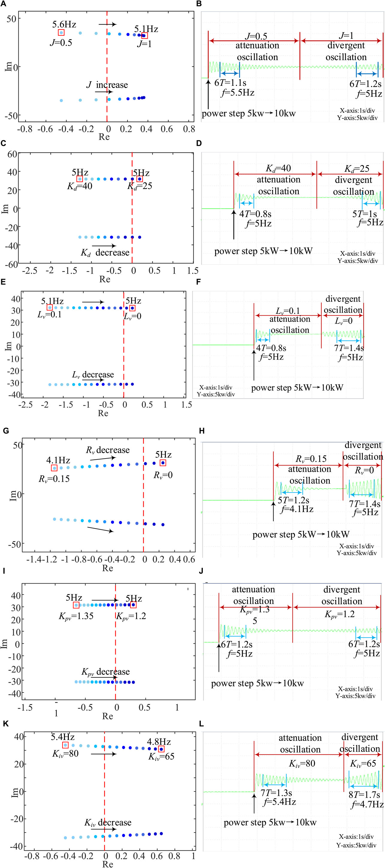
Figure 13. Experimental waveform and analysis with different parameters: (A) Eigenvalue λ_12∼13 trajectories with different J;(B) Active power experiment waveform with different J; (C) Eigenvalue λ_12∼13 trajectories with different D_p;(D) Active power experiment waveform with different D_p; (E) Eigenvalue λ_12∼13 trajectories with different L_v;(F) Active power experiment waveform with different L_v; (G) Eigenvalue λ_12∼13 trajectories with different R_v; (H) Active power experiment waveform with different R_v; (I) Eigenvalue λ_12∼13 trajectories with different K_pv;(J) Active power experiment waveform with different K_pv; (K) Eigenvalue λ_12∼13 trajectories with different K_iv; (L) Active power experiment waveform with different K_iv.

Figure 13C illustrates the variation of the eigenvalues nearest to the imaginary axis during the reduction of the virtual damping coefficient K_d from 40 to 25. From the figure, it can be found that when K_d = 40 the eigenvalues are located in the left half-plane and the system is in a stable state, which corresponds to an oscillation frequency of 5 Hz for the eigenmodes, and when K_d = 25 the eigenvalues are located in the right half-plane and the system is in a destabilized state, which corresponds to an oscillation frequency of 5 Hz for the eigenmodes. The experimental results in Figure 13D demonstrate this process; when K_d = 40, an active power step is applied and the active power oscillates with a decaying frequency of 5 Hz and the system is in a steady state. After 5 s, K_d is changed to 25, the active power oscillates with 5 Hz oscillation frequency for divergence oscillation, and the system is in the destabilized state. The experimental results are the same as the theoretical analysis, which further proves that the stability of the system deteriorates with the decrease of the virtual damping coefficient K_d in a certain range.

Figure 13E illustrates the variation of the eigenvalues nearest to the imaginary axis during the reduction of the virtual reactance L_v from 0.1 to 0. From the figure, it can be found that when L_v = 0.1 the eigenvalues are located in the left half plane and the system is in a stable state, corresponding to an oscillation frequency of the eigenmode of 5.1 Hz, and when L_v = 0 the eigenvalues are located in the right half plane and the system is in a destabilized state, corresponding to an oscillation frequency of the eigenmode of 5 Hz. The experimental results in Figure 13F demonstrate this process; when L_v = 0.1, an active power step is applied and the active power undergoes decaying oscillations at an oscillating frequency of 5 Hz and the system is in a steady state. After 5 s, L_v is changed to 0, the active power oscillates with a 5 Hz oscillation frequency for divergence oscillation, and the system is in a destabilized state. The experimental results are the same as the theoretical analysis, which further proves that the stability of the system deteriorates with the decrease of the virtual reactance L_v in a certain range.

Figure 13G illustrates the variation of the eigenvalues nearest to the imaginary axis during the reduction of the virtual resistance R_v from 0.15 to 0. From the figure, it can be found that when R_v = 0.15 the eigenvalues are located in the left half-plane and the system is in a steady state, corresponding to the eigenmode with an oscillation frequency of 4.1 Hz, and when R_v = 0 the eigenvalues are located in the right half-plane and the system is in a destabilized state, corresponding to the eigenmode with an oscillation frequency of 5 Hz.The experimental results in Figure 13H demonstrate this process, when R_v = 0.15, the application of the active power step, the active power decays and oscillates at an oscillation frequency of 4.1 Hz and the system is in a steady state. After 5 s, R_v is changed to 0, and the active power oscillates with a 5 Hz oscillation frequency for divergence oscillation, and the system is in a destabilized state. The experimental results are the same as the theoretical analysis, which further proves that the stability of the system deteriorates with the decrease of the virtual resistance R_v in a certain range.

Figure 13I illustrates the variation of the eigenvalues nearest to the imaginary axis during the reduction of the net-side voltage loop proportionality coefficient K_pv from 1.35 to 1.2. It can be found from the figure that the eigenvalues are located in the left half-plane when K_pv = 1.35, the system is in a stable state, and the corresponding eigenmode oscillates at a frequency of 5.4 Hz, and the eigenvalues are located in the right half-plane when K_pv = 1.2 and the system is in a destabilized state, and the oscillation frequency of the corresponding eigenmode is 5.4 Hz. The experimental results in Figure 13J demonstrate this process; when K_pv = 1.35, an active power step is applied and the active power undergoes decaying oscillations at an oscillating frequency of 5 Hz and the system is in a steady state. After 5 s, K_pv is changed to 1.2, the active power oscillates with 5 Hz oscillation frequency for divergence oscillation, and the coefficients are in a destabilized state. The experimental results are the same as the theoretical analysis, which further proves that the stability of the system deteriorates with the decrease of the proportionality coefficient K_pv of the grid-side voltage loop in a certain range.

Figure 13K illustrates the variation of the eigenvalue closest to the imaginary axis during the reduction of the grid-side voltage loop integration coefficient K_iv from 80 to 65. From the figure, it can be found that the eigenvalues are located in the left half-plane when K_iv = 80 and the system is in a stable state, corresponding to an oscillation frequency of the eigenmode of 5.4 Hz, and the eigenvalues are located in the right half-plane when Kiv = 65 and the system is in a destabilized state, corresponding to an oscillation frequency of the eigenmode of 4.8 Hz. The experimental results in Figure 13L demonstrate this process, when K_iv = 80, an active power step is applied and the active power oscillates decaying at a frequency of 5.4 Hz and the system is in a steady state. After 5 s, K_iv is changed to 0, the active power oscillates with a frequency of 4.7 Hz for divergence oscillation, and the system is in a destabilized state. The experimental results are the same as the theoretical analysis and simulation results, which further proves that the stability of the system deteriorates in a certain range with the decrease of the loop proportionality coefficient K_iv of the grid-side voltage.

The control parameters before and after optimization as shown in Table 3 were applied to the semi-physical simulation platform for experimental verification. We can compare the dynamic performance of the system by setting the power stepping with different short-circuit ratios. The experimental results are shown in Figure 14. From Figure 14, it can be seen that the unoptimized system has longer regulation times with larger overshoots for different grid strengths and different levels of disturbance. Moreover, the oscillations increase significantly with increasing short-circuit ratio. The optimized system shows better dynamic performance under different disturbances and different grid strengths.

Figure 14

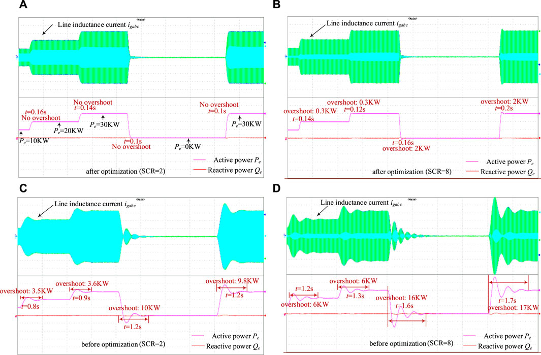
Figure 14. Experimental waveforms of active power before and after optimization for different short circuit ratios (SCR) (A) SCR = 2, after optimization (B) SCR = 8, after optimization (C) SCR = 2, before optimization (D) SCR = 8, before optimization.

7 Conclusion

The stability of single-VSG Grid-Connected system and global parameter optimization are studied in this paper. The system stability and parameter optimization methods are verified by experiments, and the following conclusions can be obtained:

(1) In the single-VSG grid-connected system, increasing the virtual inertia coefficient will rapidly reduce the damping ratio of the corresponding oscillation attenuation mode and deteriorate the system stability. Increasing the virtual damping coefficient, the virtual impedance parameters, the voltage loop proportionality coefficient and the voltage loop integration coefficient will increase the damping ratio and improve the system stability.

(2) The PSO algorithm is able to optimize all controller parameters of the system at the same time. that the optimized system has high control accuracy under different grid strengths and large disturbances, and the steady state and transient characteristics of the system are greatly improved.

Data availability statement

The raw data supporting the conclusions of this article will be made available by the authors, without undue reservation.

Author contributions

XS: Conceptualization, Writing–original draft, Writing–review and editing, Methodology. JC: Writing–review and editing, Software. DW: Writing–review and editing, Validation. JL: Writing–review and editing, Formal Analysis. KL: Writing–review and editing.

Funding

The author(s) declare that no financial support was received for the research, authorship, and/or publication of this article.

Conflict of interest

Authors XS, JC, DW, and JL were employed by Deqing Power Supply Company.

Publisher’s note

All claims expressed in this article are solely those of the authors and do not necessarily represent those of their affiliated organizations, or those of the publisher, the editors and the reviewers. Any product that may be evaluated in this article, or claim that may be made by its manufacturer, is not guaranteed or endorsed by the publisher.

Supplementary material

The Supplementary Material for this article can be found online at: https://www.frontiersin.org/articles/10.3389/fenrg.2024.1428748/full#supplementary-material

References

Baruwa, M., and Fazeli, M. (2021). Impact of virtual synchronous machines on low-frequency oscillations in power systems. IEEE Trans. Power Syst. 36, 1934–1946. doi:10.1109/TPWRS.2020.3029111

CrossRef Full Text | Google Scholar

Choopani, M., Hosseinian, S. H., and Vahidi, B. (2020). New transient stability and LVRT improvement of multi-VSG grids using the frequency of the center of inertia. IEEE Trans. Power Syst. 35, 527–538. doi:10.1109/TPWRS.2019.2928319

CrossRef Full Text | Google Scholar

Coelho, E. A. A., Cortizo, P. C., and Garcia, P. F. D. (1999). “Small signal stability for single phase inverter connected to stiff AC system,” in Conference Record of the 1999 IEEE Industry Applications Conference. Thirty-Forth IAS Annual Meeting (Cat. No.99CH36370), Phoenix, AZ, USA, 03-07 October 1999, 2180–2187. doi:10.1109/IAS.1999.798756

CrossRef Full Text | Google Scholar

D’Arco, S., and Suul, J. A. (2014). Equivalence of virtual synchronous machines and frequency-droops for converter-based MicroGrids. IEEE Trans. Smart Grid 5, 394–395. doi:10.1109/TSG.2013.2288000

CrossRef Full Text | Google Scholar

D’Arco, S., Suul, J. A., and Fosso, O. B. (2013). “Control system tuning and stability analysis of Virtual Synchronous Machines,” in 2013 IEEE energy conversion congress and exposition, Denver, CO, USA, 15-19 September 2013 (IEEE), 2664–2671. doi:10.1109/ECCE.2013.6647045

CrossRef Full Text | Google Scholar

D’Arco, S., Suul, J. A., and Fosso, O. B. (2015). Small-signal modeling and parametric sensitivity of a virtual synchronous machine in islanded operation. Int. J. Electr. Power & Energy Syst. 72, 3–15. doi:10.1016/j.ijepes.2015.02.005

CrossRef Full Text | Google Scholar

Du, W., Fu, Q., and Wang, H. (2020). Damping torque analysis of DC voltage stability of an MTDC network for the wind power delivery. IEEE Trans. Power Deliv. 35, 324–338. doi:10.1109/TPWRD.2019.2933641

CrossRef Full Text | Google Scholar

Du, Y., Guerrero, J. M., Chang, L., Su, J., and Mao, M. (2013). “Modeling, analysis, and design of a frequency-droop-based virtual synchronous generator for microgrid applications,” in 2013 IEEE ECCE Asia downunder, Melbourne, VIC, Australia, 03-06 June 2013, 643–649. doi:10.1109/ECCE-Asia.2013.6579167

CrossRef Full Text | Google Scholar

Guerrero, J. M., de Vicuna, L. G., Matas, J., Castilla, M., and Miret, J. (2004). A wireless controller to enhance dynamic performance of parallel inverters in distributed generation systems. IEEE Trans. Power Electron. 19, 1205–1213. doi:10.1109/TPEL.2004.833451

CrossRef Full Text | Google Scholar

Guerrero, J. M., Matas, J., Garcia de Vicuna, L., Castilla, M., and Miret, J. (2007). Decentralized control for parallel operation of distributed generation inverters using resistive output impedance. IEEE Trans. Industrial Electron. 54, 994–1004. doi:10.1109/TIE.2007.892621

CrossRef Full Text | Google Scholar

Li, C., Yang, Y., Cao, Y., Aleshina, A., Xu, J., and Blaabjerg, F. (2023). Grid inertia and damping support enabled by proposed virtual inductance control for grid-forming virtual synchronous generator. IEEE Trans. Power Electron. 38, 294–303. doi:10.1109/TPEL.2022.3203049

CrossRef Full Text | Google Scholar

Lu, S., Zhu, Y., Dong, L., Na, G., Hao, Y., Zhang, G., et al. (2022). Small-signal stability research of grid-connected virtual synchronous generators. Energies 15, 7158. doi:10.3390/en15197158

CrossRef Full Text | Google Scholar

Pattabiraman, D., Lasseter, R. H., and Jahns, T. M. (2018). “Comparison of grid following and grid forming control for a high inverter penetration power system,” in 2018 IEEE power & energy society general meeting (PESGM), Portland, OR, USA, 05-10 August 2018 (IEEE), 1–5. doi:10.1109/PESGM.2018.8586162

CrossRef Full Text | Google Scholar

Pogaku, N., Prodanovic, M., and Green, T. C. (2007). Modeling, analysis and testing of autonomous operation of an inverter-based microgrid. IEEE Trans. Power Electron. 22, 613–625. doi:10.1109/TPEL.2006.890003

CrossRef Full Text | Google Scholar

Wu, H., Ruan, X., Yang, D., Chen, X., Zhao, W., Lv, Z., et al. (2016). Small-signal modeling and parameters design for virtual synchronous generators. IEEE Trans. Ind. Electron. 63, 4292–4303. doi:10.1109/TIE.2016.2543181

CrossRef Full Text | Google Scholar

Wu, W., Zhou, L., Chen, Y., Luo, A., Dong, Y., Zhou, X., et al. (2019). Sequence-impedance-based stability comparison between VSGs and traditional grid-connected inverters. IEEE Trans. Power Electron. 34, 46–52. doi:10.1109/TPEL.2018.2841371

CrossRef Full Text | Google Scholar

Xiong, L., Zhuo, F., Wang, F., Liu, X., Chen, Y., Zhu, M., et al. (2016). Static synchronous generator model: a new perspective to investigate dynamic characteristics and stability issues of grid-tied PWM inverter. IEEE Trans. Power Electron. 31, 6264–6280. doi:10.1109/TPEL.2015.2498933

CrossRef Full Text | Google Scholar

Xu, Y., Nian, H., Hu, B., and Sun, D. (2021). Impedance modeling and stability analysis of VSG controlled type-IV wind turbine system. IEEE Trans. Energy Convers. 36, 3438–3448. doi:10.1109/TEC.2021.3062232

CrossRef Full Text | Google Scholar

Zhang, H., Xiang, W., Lin, W., and Wen, J. (2021). Grid forming converters in renewable energy sources dominated power grid: control strategy, stability, application, and challenges. J. Mod. Power Syst. Clean Energy 9, 1239–1256. doi:10.35833/MPCE.2021.000257

CrossRef Full Text | Google Scholar