MRGS-LSTM: a novel multi-site wind speed prediction approach with spatio-temporal correlation

The wind energy industry is witnessing a new era of extraordinary growth as the demand for renewable energy continues to grow. However, accurately predicting wind speed remains a significant challenge due to its high fluctuation and randomness. These difficulties hinder effective wind farm management and integration into the power grid. To address this issue, we propose the MRGS-LSTM model to improve the accuracy and reliability of wind speed prediction results, which considers the complex spatio-temporal correlations between features at multiple sites. First, mRMR-RF filters the input multidimensional meteorological variables and computes the feature subset with minimum information redundancy. Second, the feature map topology is constructed by quantifying the spatial distance distribution of the multiple sites and the maximum mutual information coefficient among the features. On this basis, the GraphSAGE framework is used to sample and aggregate the feature information of neighboring sites to extract spatial feature vectors. Then, the spatial feature vectors are input into the long short-term memory (LSTM) model after sliding window sampling. The LSTM model learns the temporal features of wind speed data to output the predicted results of the spatio-temporal correlation at each site. Finally, through the simulation experiments based on real historical data from the Roscoe Wind Farm in Texas, United States, we prove that our model MRGS-LSTM improves the performance of MAE by 15.43%–27.97% and RMSE by 12.57%–25.40% compared with other models of the same type. The experimental results verify the validity and superiority of our proposed model and provide a more reliable basis for the scheduling and optimization of wind farms.

1 Introduction

As a green, renewable and clean source of energy, wind energy is crucial for mitigating climate change and building a sustainable energy system. Currently, wind power has become an important part of global renewable energy (https://gwec.net/wp-content/uploads/2023/04/GWEC-2023_interactive.pdf, 2023). However, due to the high randomness and volatility of wind speed, large-scale grid-connected wind power can pose a serious threat to the smooth operation of the power systems (Zhang et al., 2019; Li, 2022). Predicting wind speed can help wind farms to adjust their scheduling plans in real time and provide a reference for the operation and maintenance time of wind turbines (Wu et al., 2021). Therefore, improving the accuracy of wind speed prediction will reduce the cost of wind energy utilization and enhance the efficiency of wind power access (Khosravi et al., 2018; Zhang et al., 2020).

Generally, wind speed prediction methods are divided into physical, statistical and machine learning methods. Physical methods use numerical weather prediction models and probability density models to correct errors. Statistical methods mainly use differential autoregressive moving average models to fit historical data (Cadenas et al., 2016), but both of these methods cannot well capture the dynamic changes and nonlinear features of wind speed. Machine learning methods have been widely used in the field of wind speed prediction for single turbines because of their powerful feature extraction capabilities. Time-series prediction models such as LSTM (Liu et al., 2018; Li et al., 2022; Wang et al., 2023), gated recurrent unit (GRU) (Li et al., 2020; Wang and Gui, 2022) etc. have strong nonlinear fitting effects and strong learning ability, which in turn are more popular in wind speed prediction modeling. For example, Wu et al. (2021) proposed an LSTM network model that combines the maximum information coefficient (MIC) and multi-task learning, and verified that the machine learning model outperforms physical and statistical methods. Chen et al. (2021) leveraged bidirectional GRU to improve the accuracy and generalization ability of the model by extracting the temporal feature information of wind power and meteorological data. From a macroscale perspective, wind speed exhibits certain regularities and periodicities annually, quarterly, and even monthly. In addition, studies (Nielson and Bhaganagar., 2019; Nielson et al., 2020) have shown that atmospheric stability plays a key role in wind energy production. Considering atmospheric input characteristics, such as wind shear and turbulence intensity, can significantly improve the accuracy of wind turbine power predictions. This highlights the importance of including atmospheric variables in wind speed prediction models to improve their performance and reliability.

Wind farms are mostly constructed in clusters, and single turbine wind speed prediction methods are more difficult to adapt to wind speed prediction scenarios in wind farms. Due to the high similarity of the environment and meteorological conditions in which the wind farms are located, there is also a correlation between the wind speed variations among the sites within the wind farms, and this spatial correlation can be utilized to improve the accuracy of wind speed prediction. Zhu et al. (2021) used convolutional neural network (CNN) to extract the field-wide features that affect the long-term wind speed distribution and considered the wind speed correlation among units. However, the single feature limits the ability of the model to capture complex interactions in the multi-turbine feature expansion. Wang et al. (2022) proposed an ultra-short-term wind farm cluster power forecasting method based on dynamic spatio-temporal correlation. Yu et al. (2022) established a CNN-LSTM-AM dynamic integration model. But CNN could not accurately express the spatial features of wind field distributed by non-grid structure, which resulted in low accuracy of wind speed prediction. Bai et al. (2024) proposed a wind speed prediction model based on the improved variational mode decomposition and Seq2Seq network, which fully learns the implicit correlation features of multidimensional time series data. Meanwhile, the Seq2Seq model has a complex encoder and decoder structure, which makes the model consume a large number of computational resources when the wind speed fluctuates greatly. On the whole, the above methods fail to fully utilize the spatial correlation of multi-variables among sites within a wind farm, and the spatial relationship of multi-variables is insufficiently portrayed.

In recent years, there has been an increasing trend in researches on modeling spatial features using graph models to characterize the spatial correlation of multiple wind farm features. The spatial relationships between nodes are characterized by graph models, which are used for feature transfer and aggregation to better extract spatial features via graph neural network (GNN). Typical graph neural networks are GCN (Liu and Ware, 2022), GAT (Liu et al., 2023a), etc., which have been successfully applied to extract spatial features from graph models in various fields, such as traffic prediction (Yu et al., 2018) and airport delay prediction (Zeng et al., 2021). Geng et al. (2021) proposed a graph optimization neural network for multi-node offshore wind speed prediction, which captures spatial dependencies and generates high-dimensional spatial features through GCN and channel attention mechanisms. Khodayar and Wang (2019) combined rough set networks and GCN to extract spatial features of wind farms. Liu et al. (2023b) proposed an adaptive graph learning convolutional network (AGLCN) that can automatically infer hidden associations and achieve better results in extracting spatial features of offshore wind farms. He et al. (2022) used GAT to extract multi-site wind features for collaborative wind speed prediction to improve the accuracy of model. Therefore, wind speed prediction of multiple sites requires comprehensive consideration of both time-series data from each individual site as well as interactions between their respective distributions across space. Reasonably and efficiently characterizing and utilizing this spatial and temporal correlations of multiple sites are the key to improving the accuracy of wind speed prediction model. Many studies either focus on single turbine wind prediction or fail to adequately capture the complex spatio-temporal interactions within sites. Moreover, traditional models often overlook the irregular distribution of wind turbines, resulting in poor generality in practical applications.

The main idea of this study is to propose a novel wind speed prediction model, called MRGS-LSTM, which integrates the spatio-temporal correlation of irregular multiple sites distributions. The novelty and contributions of this study are described below.

1. We randomly select 20 irregularly distributed wind turbines to validate our model’s robustness in handling datasets from irregular wind site layouts.

2. We develop a novel mRMR-RF method to assess the importance of various features and select the most influential subset relevant to wind speed prediction.

3. Our innovative MRGS-LSTM model extracts spatio-temporal features from multiple sites. Experiments show that central sites achieve better prediction accuracy by incorporating wind speed data from neighboring sites.

4. We selected other mainstream graph neural network models and temporal feature extraction models to construct 5 comparison models. The experimental results show that our model has excellent performance in MAE and RMSE.

2 Methodology

2.1 Graph modeling

Assuming that a graph, $G=\left(V,E\right)$, where $V$ represents the set of $N$ nodes, and $E$ is the set of edges that show the node-to-node connectivity. Node $V_i$ and $V_j$ are connected in the graph only when there exists a strong correlation between them, where $V_i,V_j\in V,i,j\in \left\{1,2,...,N\right\}$. The correlation between $V_i$ and $V_j$ is defined as $r_{V_i{V}_j}$. $X=\left\{X^1,X^2,...,X^N\right\}$, where $X^i=\left\{x_1^i,x_2^i,...,x_n^i\right\}$ is the feature set with number n of node $V_i$, denotes the sample set of all nodes. $W$ is a $N\times N$ adjacency matrix. To enhance computational efficiency of graph neural networks and prevent interference from weakly correlated nodes, $W_{ij}$ is defined as Equation 1.

${\mathit{W}}_{\mathit{i}\mathit{j}}=\left\{\begin{array}{c}{\mathit{r}}_{{\mathit{V}}_{\mathit{i}}{\mathit{V}}_{\mathit{j}}},{\mathit{r}}_{{\mathit{V}}_{\mathit{i}}{\mathit{V}}_{\mathit{j}}}\ge \mathbf{0.8}\\ \mathbf{0},\mathit{o}\mathit{t}\mathit{h}\mathit{e}\mathit{r}\mathit{w}\mathit{i}\mathit{s}\mathit{e}\end{array}\right.,(1)$

where $W_{ij}=W_{ji}$. Figure 1 shows an example of adjacency matrix construction, which describes the connection relationships and correlations between nodes.

Figure 1

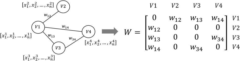
Figure 1. Adjacency matrix construction.

2.1.1 GraphSAGE

GraphSAGE network is an inductive learning framework for graph representation. By leveraging the attribute information of the nodes, this network can efficiently generate vector representations of unknown nodes or new graphs. Computational complexities are reduced by sampling neighboring nodes for aggregated representation. GraphSAGE can also capture diverse graph structures and feature information to fit various graph data and tasks.

GraphSAGE randomly samples the target nodes with K layers of neighbor nodes. The preset number of neighbor nodes to be sampled in each layer is denoted as $S_k,k=1,2,...,K$. During sampling, if the node number of the $k$-th layer is less than $S_k$, the sampling scheme without replacement is adopted, otherwise the sampling scheme with replacement is utilized. Based on the study by Hamilton et al. (2018), we select K = 2 for GraphSAGE to achieve excellent performance. For example, if $S_1$ = 3 and $S_2$ = 7, the sampling and aggregation process is shown in Figure 2. The blue dots and the green dots represent the first-order and second-order neighbor node sampled for the target node, respectively.

Figure 2

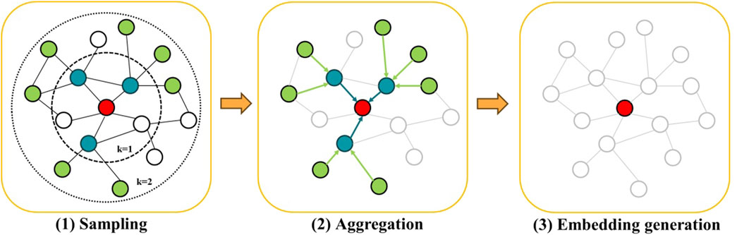
Figure 2. Illustration of GraphSAGE.

GraphSAGE aggregates the information of neighboring nodes at each layer through the aggregation function AGGREGATE. Afterwards, the information of the target node is continuously updated by Equations 2, 3.

${{\mathit{h}}_{\mathit{N}\left(\mathit{V}\right)}^{\mathit{k}}\leftarrow \mathit{A}\mathit{G}\mathit{G}\mathit{R}\mathit{E}\mathit{G}\mathit{A}\mathit{T}\mathit{E}}^{\mathit{k}}\left(\left\{{\mathit{h}}_{\mathit{u}}^{\mathit{k}-\mathbf{1}},\forall \mathit{u}\in \mathit{N}\left(\mathit{V}\right)\right\}\right),(2)$

${\mathit{h}}_{\mathit{V}}^{\mathit{k}}\leftarrow \mathit{\sigma }\left({\mathit{Z}}^{\mathit{k}}·\mathit{C}\mathit{O}\mathit{N}\mathit{C}\mathit{A}\mathit{T}\left({\mathit{h}}_{\mathit{V}}^{\mathit{k}-\mathbf{1}},{\mathit{h}}_{\mathit{N}\left(\mathit{V}\right)}^{\mathit{k}}\right)\right),(3)$

where $N\left(V\right)$ denotes the set of neighbor nodes of node V, $h_V^k$ denotes the embedding vector of node $V$ in the $k$-th epoch, the CONCAT function linearly superimposes each vector using residual crosstabs, $Z^k$ is the weight matrix that GraphSAGE needs to learn, and $\sigma$ is the nonlinear activation function ReLU, which can effectively solve the vanishing gradient problem and improve the convergence speed of the network. To increase the convergence of the model, vector representation can be normalized by Equation 4.

${\mathit{h}}_{\mathit{V}}^{\mathit{k}}\leftarrow \frac{{\mathit{h}}_{\mathit{V}}^{\mathit{k}}}{{‖{\mathit{h}}_{\mathit{V}}^{\mathit{k}}‖}^{\mathbf{2}}}.(4)$

2.2 LSTM

Memory cell units are incorporated in the hidden layers for LSTM to realize the selective memory and forgetting of information and retain a certain length of historical information. Notably, LSTM excels in capturing long-term dependency in data and solves the problems of gradient vanishing and gradient explosion. Figure 3 illustrates the LSTM network structure, which contains multiple memory cells. Furthermore, each cell is extended with an input gate, a forget gate and an output gate.

Figure 3

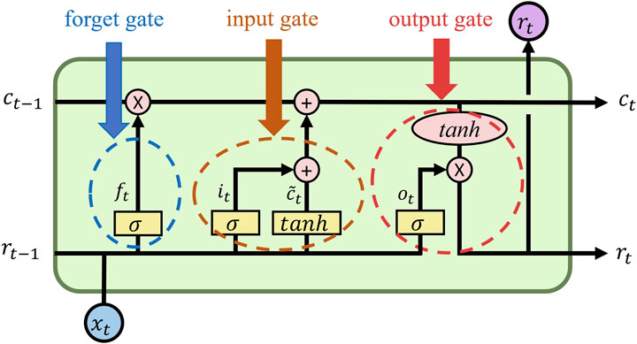
Figure 3. LSTM network structure.

Input gate: The input gate $i_t$ regulates the inclusion of new inputs according to the hidden state of the previous period and the inputs of the current period. Additionally, the cell state ${\stackrel{\sim }{c}}_t$ selectively stores the input information. The calculation of the input gate and the cell state are as follows by Equations 5, 6.

${\mathit{i}}_{\mathit{t}}=\mathit{\sigma }\left({\mathit{\omega }}_{\mathit{i}}·\left[{\mathit{r}}_{\mathit{t}-\mathbf{1}},{\mathit{x}}_{\mathit{t}}\right]+{\mathit{b}}_{\mathit{i}}\right),(5)$

${\stackrel{\sim }{\mathit{c}}}_{\mathit{t}}=\mathit{tanh}\left({\mathit{\omega }}_{\mathit{c}}·\left[{\mathit{r}}_{\mathit{t}-\mathbf{1}},{\mathit{x}}_{\mathit{t}}\right]+{\mathit{b}}_{\mathit{c}}\right).(6)$

where $r_{t-1}$ denotes the hidden state of the previous period, $x_t$ denotes the inputs of the current period, $\omega$ is the weight coefficients, and b is the bias values, $\sigma$ and tanh denote the sigmoid activation function and hyperbolic tangent function respectively.

Forget gate: The forget gate $f_t$ determines the selective forgetting or retention of the previous output information. The forget gate is calculated according to the following Equation 7.

${\stackrel{\sim }{\mathit{c}}}_{\mathit{t}}=\mathit{tanh}\left({\mathit{\omega }}_{\mathit{c}}·\left[{\mathit{r}}_{\mathit{t}-\mathbf{1}},{\mathit{x}}_{\mathit{t}}\right]+{\mathit{b}}_{\mathit{c}}\right).(7)$

Output gate: The output gate $o_t$ obtains the output of the LSTM network according to the cell state $c_t$. The calculation of the output gate can be expressed as Equations 8, 9.

${\mathit{o}}_{\mathit{t}}=\mathit{\sigma }\left({\mathit{\omega }}_{\mathit{o}}·\left[{\mathit{r}}_{\mathit{t}-\mathbf{1}},{\mathit{x}}_{\mathit{t}}\right]+{\mathit{b}}_{\mathit{o}}\right),(8)$

${\mathit{r}}_{\mathit{t}}={\mathit{o}}_{\mathit{t}}\odot \mathit{tanh}\left({\mathit{c}}_{\mathit{t}}\right),(9)$

where $\odot$ denotes the Hadamard product. Based on the aforementioned calculation results, the cell state is updated by Equation 10.

${\mathit{c}}_{\mathit{t}}={\mathit{f}}_{\mathit{t}}\odot {\mathit{c}}_{\mathit{t}-\mathbf{1}}+{\mathit{i}}_{\mathit{t}}\odot {\stackrel{\sim }{\mathit{c}}}_{\mathit{t}}.(10)$

3 Spatial feature extraction

3.1 mRMR

Assuming that the original dataset of a wind farm with N sites is $X=\left\{X^1,X^2,...,X^N\right\}$, where $X^j=\left\{{\chi }_1^j,{\chi }_2^j,...,{\chi }_n^j\right\}$ denotes the feature set of site j, ${\chi }_i^j=\left[x_i^j\left(1\right),x_i^j\left(2\right),\dots ,x_i^j\left(M\right)\right]$ is the i-th feature sequence of site j, the feature vector ${\gamma }_i=\left[{\chi }_i^1,{\chi }_i^2,\dots ,{\chi }_i^N\right]$ is constructed by concatenating the i-th feature values of all sites. The minimum redundancy maximum relevance (mRMR) algorithm assesses the significance of features by quantifying the correlation between each feature and the target variable, as shown in Equation 11.

$\mathit{I}\left({\mathit{\gamma }}_{\mathit{i}};{\mathit{\gamma }}_{\mathit{j}}\right)=\iint \mathit{p}\left({\mathit{\gamma }}_{\mathit{i}},{\mathit{\gamma }}_{\mathit{j}}\right){\mathit{log}}_{\mathbf{2}}\frac{\mathit{p}\left({\mathit{\gamma }}_{\mathit{i}},{\mathit{\gamma }}_{\mathit{j}}\right)}{\mathit{p}\left({\mathit{\gamma }}_{\mathit{i}}\right)\mathit{p}\left({\mathit{\gamma }}_{\mathit{j}}\right)}\mathit{d}{\mathit{\gamma }}_{\mathit{i}}\mathit{d}{\mathit{\gamma }}_{\mathit{j}},(11)$

where $\mathit{p}\left(·\right)$ is the probability distribution function. The mRMR algorithm consists of two parts:

Max Relevance: Define S as the feature subset of ${\gamma }_i$. Average the summation of the relevance between each feature and the target, as shown in Equation 12.

${\mathit{D}}_{\mathit{i}}=\frac{\mathbf{1}}{\left|\mathit{S}\right|}{\displaystyle {\sum }_{{\mathit{\gamma }}_{\mathit{i}}\in \mathit{S}}}\mathit{I}\left({\mathit{\gamma }}_{\mathit{i}};\mathit{c}\right),(12)$

where $\left|\mathit{S}\right|$ denotes the dimension of the feature subset and c denotes the target.

Minimum Redundancy: Calculate the redundancy between the features, as shown in Equation 13.

${\mathit{R}}_{\mathit{i}}=\frac{\mathbf{1}}{{\left|\mathit{S}\right|}^{\mathbf{2}}}{\displaystyle {\sum }_{{\mathit{\gamma }}_{\mathit{i}},{\mathit{\gamma }}_{\mathit{j}}\in \mathit{S}}}\mathit{I}\left({\mathit{\gamma }}_{\mathit{i}};{\mathit{\gamma }}_{\mathit{j}}\right),(13)$

3.2 mRMR-RF

Random forest (RF) is an integrated machine learning algorithm. Multiple decision tree model, which is the supervised learning algorithm, improves the accuracy and stability of feature selection. By using mutual information as metric and considering that both feature relevance and redundancy, mRMR can be embedded into RF to select feature subsets with minimal information redundancy which can effectively eliminate irrelevant or repetitive features. As illustrated in Figure 4, the specific processes are as follows:

Figure 4

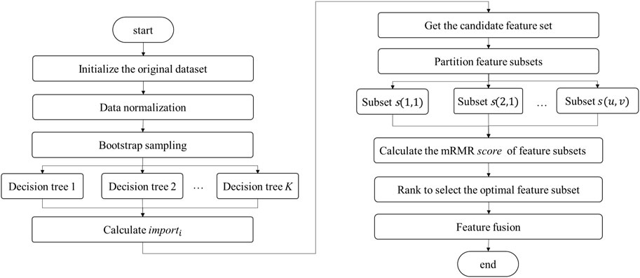
Figure 4. mRMR-RF feature selection.

Initialize the original dataset: The original dataset is divided into features and target.

Data normalization: The constructed dataset is normalized to eliminate the influence of dimensions by Equation 14.

${\widehat{\mathit{\gamma }}}_{\mathit{i}}=\frac{{\mathit{\gamma }}_{\mathit{i}}-{\mathit{\gamma }}_{\mathit{i},\mathit{min}}}{{\mathit{\gamma }}_{\mathit{i},\mathit{max}}-{\mathit{\gamma }}_{\mathit{i},\mathit{min}}},(14)$

where ${\widehat{\gamma }}_i$ is the normalized data, ${\gamma }_{i,\mathit{min}}$ and ${\gamma }_{i,\mathit{max}}$ are the maximum and minimum values of the feature data, respectively.

Bootstrap Sampling: Sample data are randomly drawn with replacement from the feature to build K decision trees. If the feature has M points, then the unsampled probability of each record is $P={\left(1-\frac{1}{M}\right)}^M$. When $\underset{M\to \infty }{\lim }P=1/e$, 36.8% of features are not included in the training set. These data are also called Out-Of-Bag data (OOB data).

Getting the candidate feature set: The error values ${Err}_i\left(j\right)\left(j=1,2,...,K\right)$ for each decision tree are calculated from the OOB data$.$ RF shuffles the feature ${\gamma }_i$ in the OOB data and recalculates the error values ${Err}_i^{*}\left(j\right)$. The equation for calculating the feature importance is shown as Equation 15.

${\mathit{i}\mathit{m}\mathit{p}\mathit{o}\mathit{r}\mathit{t}}_{\mathit{i}}=\frac{\mathbf{1}}{\mathit{K}}{\displaystyle {\sum }_{\mathit{j}=\mathbf{1}}^{\mathit{K}}}\left[{\mathit{E}\mathit{r}\mathit{r}}_{\mathit{i}}\left(\mathit{j}\right)-{\mathit{E}\mathit{r}\mathit{r}}_{\mathit{i}}^{*}\left(\mathit{j}\right)\right].(15)$

Afterwards, by ranking the feature importance, the features with high importance are filtered by the determined threshold $\epsilon$ as a candidate feature set.

Partitioning feature subsets: All possible feature subsets s(u, v) are exhaustively enumerated from the candidate feature set, where $u=1,2,...,n$ is the number of features in the subset, $v=1,2,...,{\sum }_{u=1}^N{C}_n^u$ is the number of subsets.

Calculating the mRMR score of feature subsets: Calculate the score of the feature subset s(u, v) via the following Equation 16:

${\mathit{s}\mathit{c}\mathit{o}\mathit{r}\mathit{e}}_{\left(\mathit{u},\mathit{v}\right)}={\displaystyle {\sum }_{\mathit{i}=\mathbf{1}}^{\mathit{u}}}{\mathit{D}}_{\mathit{i}}-{\displaystyle {\sum }_{\mathit{i}=\mathbf{1}}^{\mathit{u}}}{\mathit{R}}_{\mathit{i}}.(16)$

The optimal feature subset is selected by ranking each feature subset score.

Feature fusion: The fused feature ${\widehat{X}}^j$ of site j is obtained by averaging the selected optimal feature subset. $\widehat{X}=\left\{{\widehat{X}}^1,{\widehat{X}}^2,...{,\widehat{X}}^N\right\}$ denotes the fused feature of all sites. The process of feature fusion is shown as Equation 17.

${\widehat{\mathit{X}}}^{\mathit{j}}=\frac{\mathbf{1}}{\mathit{u}}{\sum }_{\mathit{i}=\mathbf{1}}^{\mathit{u}}{\widehat{\mathit{\chi }}}_{\mathit{i}}^{\mathit{j}}.(17)$

3.3 Topology construction of spatial features

The graph structured data represent the multi-site features and their correlations. N sites and their feature correlation are topologically constructed as Equation 18.

$\mathit{G}=\left(\mathit{V},\mathit{E},\widehat{\mathit{X}},\mathit{W}\right),(18)$

where $V=\left\{V_1,V_2,...,V_N\right\}$ denotes the set of sites, E denotes the set of edges formed between sites, $\widehat{X}$ represents the fused features of all sites, and $W\in R^{N\times N}$ is the weighted adjacency matrix, which is constructed by concurrently considering the spatial distance correlation and time series correlation among multi-site. The spatial weighted adjacency matrix $W^{space}$ and the temporal weighted adjacency matrix $W^{time}$ individually express the correlations. Subsequently, we linearly weighted the sum of both to obtain the weighted adjacency matrix W, as shown in Equation 19.

$\mathit{W}={\mathit{\alpha }\mathit{W}}^{\mathit{s}\mathit{p}\mathit{a}\mathit{c}\mathit{e}}+\left(\mathbf{1}-\mathit{\alpha }\right){\mathit{W}}^{\mathit{t}\mathit{i}\mathit{m}\mathit{e}},(19)$

where $\alpha \in \left[0,1\right]$ is a weighting parameter.

Spatial distance correlation: The wind speeds at adjacent sites are correlated due to the influence of the internal atmosphere of the region. Generally, the closer the distance between two sites is, the stronger the correlation between sites is, and vice versa. Therefore, we take the actual longitude and latitude of sites as inputs and use the Haversine formula to calculate the spherical distance between sites. If the distance is less than or equal to a threshold parameter $\theta$, then we use the Gaussian kernel function to calculate the spatial distance correlation. Otherwise, it indicates that there is no spatial distance correlation between them. For any two sites $V_i$ and $V_j$, the edge weight is calculated according to the following Equation 20.

${\mathit{w}}_{\mathit{i}\mathit{j}}^{\mathit{s}\mathit{p}\mathit{a}\mathit{c}\mathit{e}}=\left\{\begin{array}{c}\mathit{exp}\left(-\frac{{\left(\mathit{d}\mathit{i}\mathit{s}\mathit{t}\left({\mathit{V}}_{\mathit{i}},{\mathit{V}}_{\mathit{j}}\right)\right)}^{\mathbf{2}}}{\mathbf{2}{\mathit{\sigma }}^{\mathbf{2}}}\right),\mathit{i}\mathit{f}\mathit{d}\mathit{i}\mathit{s}\mathit{t}\left({\mathit{V}}_{\mathit{i}},{\mathit{V}}_{\mathit{j}}\right)\le \mathit{\theta }\\ \mathbf{0},\mathit{o}\mathit{t}\mathit{h}\mathit{e}\mathit{r}\mathit{w}\mathit{i}\mathit{s}\mathit{e}\end{array}\right.,(20)$

where $dist\left(V_i,V_j\right)$ represents the spherical distance between nodes $V_i$ and $V_j$ and $\sigma$ is the standard deviation of $dist\left(V_i,V_j\right)$.

Time series correlation: The wind speeds between multiple sites are affected not only by the spatial distance, but also by the similarity of their time series. If the wind speeds of two sites are closer to each other at the same time, the time series correlation will be stronger. Due to the nonlinearity of the wind speed series, we adopt MIC to grid partition the data space. The mutual information between $V_i$ and $V_j$ and their normalized edge weights are as follows by Equations 21, 22.

$\mathit{I}\left({\mathit{V}}_{\mathit{i}};{\mathit{V}}_{\mathit{j}}\right)=\iint \mathit{p}\left({\widehat{\mathit{X}}}^{\mathit{i}},{\widehat{\mathit{X}}}^{\mathit{j}}\right){\mathit{log}}_{\mathbf{2}}\frac{\mathit{p}\left({\widehat{\mathit{X}}}^{\mathit{i}},{\widehat{\mathit{X}}}^{\mathit{j}}\right)}{\mathit{p}\left({\widehat{\mathit{X}}}^{\mathit{i}}\right)\mathit{p}\left({\widehat{\mathit{X}}}^{\mathit{j}}\right)}\mathit{d}{\widehat{\mathit{X}}}^{\mathit{i}}\mathit{d}{\widehat{\mathit{X}}}^{\mathit{j}},(21)$

${\mathit{w}}_{\mathit{i}\mathit{j}}^{\mathit{t}\mathit{i}\mathit{m}\mathit{e}}=\mathit{M}\mathit{I}\mathit{C}\left({\mathit{V}}_{\mathit{i}};{\mathit{V}}_{\mathit{j}}\right)={\mathit{max}}_{\left|{\widehat{\mathit{X}}}^{\mathit{i}}\right|\left|{\widehat{\mathit{X}}}^{\mathit{j}}\right|<\mathit{B}}\frac{\mathit{I}\left({\mathit{V}}_{\mathit{i}};{\mathit{V}}_{\mathit{j}}\right)}{{\mathit{log}}_{\mathbf{2}}\left(\mathit{min}\left(\left|{\widehat{\mathit{X}}}^{\mathit{i}}\right|,\left|{\widehat{\mathit{X}}}^{\mathit{j}}\right|\right)\right)}.(22)$

where $MIC\left(V_i;V_j\right)$ is the maximum information coefficient between nodes and B is the number of grids, which is generally taken as the total amount of data 0.6 times (Chen et al., 2016).

3.4 mRMR-RF-GraphSAGE

The specific processes of the spatial feature extraction framework based on mRMR-RF-GraphSAGE are as follows:

(1) Use mRMR-RF to filter the most representative and distinguishable optimal feature subset, effectively reducing the original feature data dimensionality and complexity. Feature fusion is then applied to synthesize the selected features into a comprehensive representation;

(2) Construct the spatial feature map topology by integrating location information from multi-site, thereby transforming the data into a graph structured format. The spatial feature map serves as a topological representation of features to convey the geographical relationships and time series correlations between different sites;

(3) Utilize the GraphSAGE to train the graph structured data to generate embedding spatial feature vectors by sampling and aggregating neighbor information, which can fully explore the potential of graph structured data.

4 Spatio-temporal feature extraction framework

The framework proposed in this paper for spatio-temporal feature extraction is articulated into four main components: data preparation, multi-site map topology construction, spatial feature extraction and temporal feature extraction, as illustrated in Figure 5.

Figure 5

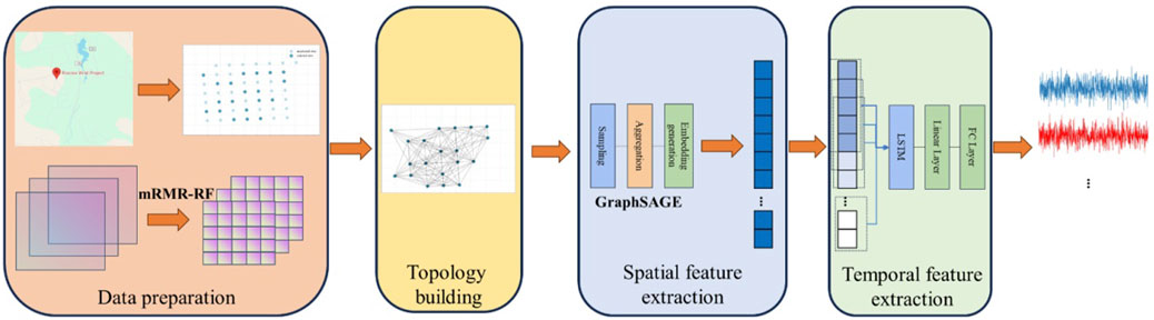
Figure 5. Spatio-temporal feature extraction framework.

Data preparation: We gather and systematically arrange the geographic location of multi-site, historical wind speed records and other environmental feature data. Using the mRMR-RF method, we select the optimal features to reduce the dimensionality of the original data. The final fused feature is obtained for wind speed prediction by the optimal subset.

Multi-site map topology construction: By utilizing the fused feature, we construct graph structure data that comprehensively incorporates spatial geographic information from multi-site. Each site is depicted as a node, while the edges quantify the spatial distance and time series correlation between sites. Afterwards, the weighted adjacency matrix W is constructed by combining the spatial correlation matrix $W^{space}$ based on the Haversine formula, with the time series correlation matrix $W^{time}$ derived from the MIC.

Spatial feature extraction: We utilize GraphSAGE to extract spatial features from the multi-site map topology. The uniform sampling and mean aggregation approaches are adopted to sample and aggregate neighboring sites, which yields the feature representation of the central site. Then, the spatial feature representations for each site are generated by a fully connected layer, which captures the complex spatial correlations among multiple sites.

Temporal feature extraction: The spatial feature vectors are temporally resampled using the sliding window method to generate spatio-temporal feature vectors. Subsequently, LSTM is employed for extracting temporal correlation information. The LSTM hidden layer consists of 64 nodes and the time window sampling step is set to 24. Finally, a linear layer and a fully connected layer are utilized to output the predicted values of multiple sites, thereby completing the construction of the spatio-temporal feature extraction framework.

5 Case analysis

5.1 Simulation experiment setting

This simulation experiment is implemented in Python 3.11, using an open-source machine learning platform that includes a GPU-accelerated version of the PyTorch 2.1.1 framework. This platform utilizes CUDA and cuDNN to optimize training and inference speed for deep neural networks, fully exerting the computational power of the GPU. The simulation hardware platform settings: CPU is Intel i7-13620H 2.4GHz, RAM is 16GB, and GPU is NVIDIA GeForce RTX 4060 8 GB. To prevent overfitting, we make adjustments by randomly shuffling the order of the input samples. Additionally, a fixed random seed is set to ensure reproducibility by eliminating potential impacts from random factors in deep learning models. The model training is set to 200 epochs, with a batch size of 72. The training minimizes the loss through the mean absolute error (MAE) approach and Adam optimizer while setting the weight decay at ${10}^{-5}$ (Kingma and Ba, 2017).

5.2 Evaluation metrics

In this study, the mean absolute error (MAE) and root mean square error (RMSE) are selected as model evaluation metrics. The calculation formulas of MAE and RMSE are as follows by Equation 23, 24.

$\mathit{M}\mathit{A}\mathit{E}=\frac{\mathbf{1}}{\mathit{n}}{\displaystyle {\sum }_{\mathit{i}=\mathbf{1}}^{\mathit{n}}}\left|{\mathit{y}}_{\mathit{i}}-{\widehat{\mathit{y}}}_{\mathit{i}}\right|,(23)$

$\mathbf{\text{RMSE}}=\sqrt{\frac{\mathbf{1}}{\mathbf{n}}{\displaystyle {\sum }_{\mathbf{i}=\mathbf{1}}^{\mathbf{n}}}{\left({\mathbf{y}}_{\mathbf{i}}-{\widehat{\mathbf{y}}}_{\mathbf{i}}\right)}^{\mathbf{2}}},(24)$

where $y_i$ is the true observed value of wind speed, ${\widehat{y}}_i$ is the model output predicted value of wind speed, and $n$ is the total number of data samples.

5.3 Data description

The wind energy integrated national dataset is sourced from the National Renewable Energy Laboratory (NREL) in the United States (Jager and Andreas, 1996). This dataset includes meteorological conditions at different height positions for more than 2,488,136 sites in the continental United States for the years 2007–2014. The dataset features 2 km spatial resolution and 15-min temporal resolution. This dataset consists of 32 sets of features as shown in Table 1, including information such as wind speed, wind direction, temperature and air pressure. The selected dataset for this study comes from 49 sites within the Roscoe Wind Farm area in Texas, United States, and covers the entire year of 2014. However, it should be noted that while wind turbines are typically arranged in a regular rectangular grid pattern within a wind farm, most turbines have an irregular distribution shape. Therefore, we randomly selected 20 sites with uneven distributions from all available sites as shown in Figure 6. The dataset is divided into three parts. Data from January to October 2014 was used as the training set for model training. This period was chosen to provide sufficient training data for the model. Data from November 2014 was used as the test set to evaluate the generalization ability of the final model. Data from December 2014 was used as the validation set. It help our model fine-tune to find the optimal hyperparameters and prevent overfitting.

Table 1

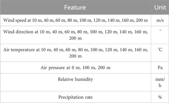
Table 1. Statistical data of the wind station features.

Figure 6

Figure 6. Schematic diagram of the multi-site location.

5.4 Experimental results and analysis

5.4.1 Feature selection analysis

Utilizing the mRMR-RF feature selection algorithm, we initially compute the RF feature importance, filtering out features with an importance greater than the threshold ($\mathrm{\epsilon }$ = 0.01). These features are exhaustively combined to form feature subsets, and calculate their mRMR scores. As a result, we identify the optimal feature subset with a high correlation to wind speed prediction. As illustrated in Figure 7, these features include wind speed at heights of 80 m, 60 m, 140 m, and 160 m. It is also evident from this process that other features were not selected due to their lower correlation with wind speed prediction.

Figure 7

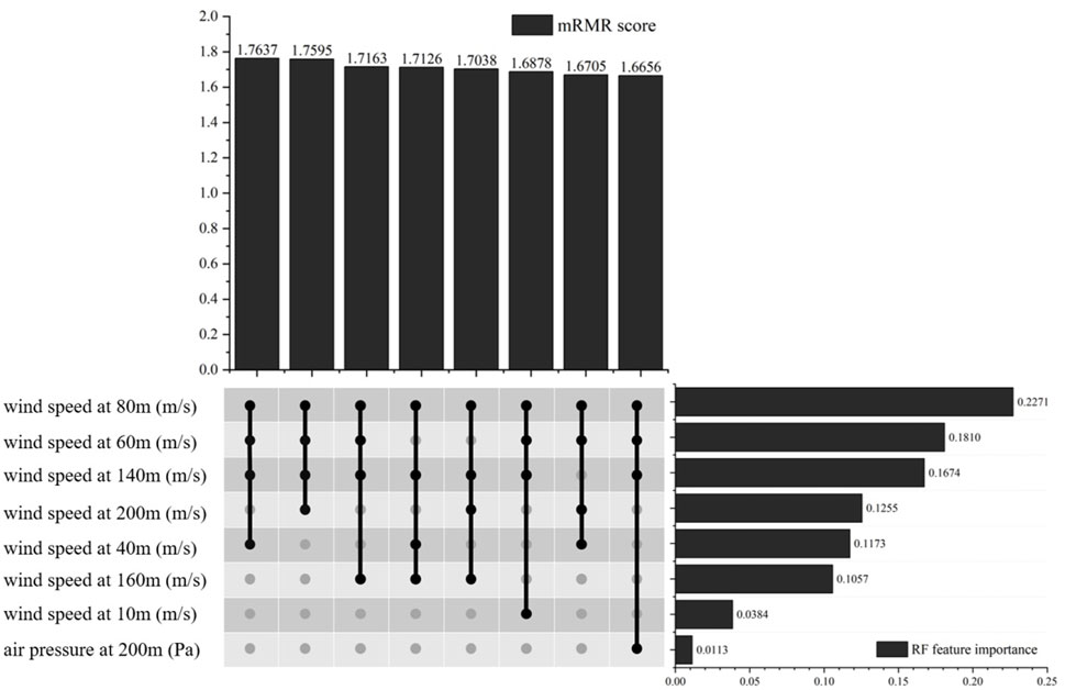
Figure 7. Importance ranking of wind site features.

5.4.2 Parameter analysis in map topology construction

In map topology construction, the threshold parameter $\theta$ and the weighting parameter $\alpha$ can influence the constructed graph structure data. The threshold parameter $\theta$ is selected from the distance between the two nearest sites to the distance between the two farthest sites, with a step length of 1 km. The weighting parameter $\alpha$ is chosen from 0 to 1, with a step length of 0.05. The optimal parameters are obtained through exhaustive searching are $\theta$ = 8 km and $\alpha$ = 0.4. The constructed topology of the multi-site is shown in Figure 8.

Figure 8

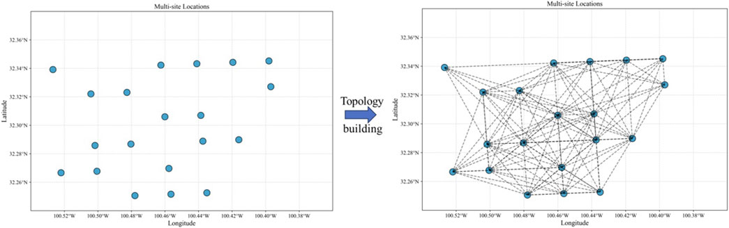
Figure 8. Multi-site topology construction.

5.4.3 Baseline model

In order to validate the efficacy and superiority of the proposed MRGS-LSTM wind speed prediction model, we conducted a comparative analysis with several widely adopted wind speed prediction algorithms. Afterwards, algorithm selection was performed by comparing various graph neural networks, namely GCN, GAT, and GraphSAGE. For time series prediction evaluation, multilayer perceptron (MLP) and LSTM were compared.

In this paper, we conducted comparative experiments on GCN-MLP, GAT-MLP, GS-MLP, GCN-LSTM, GAT-LSTM, and MRGS-LSTM. Table 2 lists the MAEs and RMSEs of wind speed prediction for these models. The min, max, average and std are the minimum, maximum, mean and standard deviation of the prediction error for all the sites, respectively. To better evaluate the improvement effect of MRGS-LSTM compared with other prediction models, the calculation formula of imp is as follows by Equation 25.

$\mathit{i}\mathit{m}\mathit{p}=\frac{\left|{\mathit{E}}_{\mathit{o}}-{\mathit{E}}_{\mathit{p}}\right|}{{\mathit{E}}_{\mathit{o}}}\times \mathbf{100}\%,(25)$

where $imp$ denotes the average improvement value of wind speed accuracy for our model compared to the comparison models, $E_o$ is the error value of the comparison models, and $E_p$ is the error value of our model.

Table 2

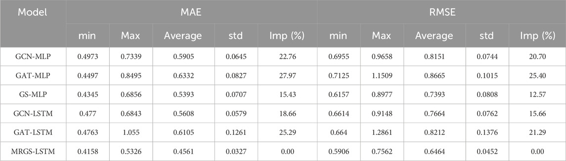
Table 2. Comparison of the wind speed prediction errors of multiple sites.

The minimum value of the error for these models is indicated in bold in the Table 2. Our proposed MRGS-LSTM model in this study exhibits the smallest MAE and RMSE values, outperforming all other prediction models. Compared to GCN-MLP, GAT-MLP, and GS-MLP which do not incorporate temporal features, MRGS-LSTM achieves 22.76%, 27.97%, and 15.43% improvements in the statistical mean of MAE respectively, as well as 20.70%, 25.40%, and 12.57% improvements in the statistical mean of RMSE respectively. Furthermore, when compared to GCN-LSTM and GAT-LSTM, which utilize other GNNs for spatial feature extraction, MRGS-LSTM improves the mean MAE by 18.66% and 25.29%, respectively, and improves the mean RMSE by 15.66% and 21.29%, respectively. Moreover, using MRGS-LSTM for wind speed prediction, the error ranges of MAE and RMSE are between 0.4158 m/s and 0.5326 m/s and between 0.5906 m/s and 0.7562 m/s, respectively. Also, the average and std are significantly smaller than those obtained from other prediction models. This confirms that our proposed MRGS-LSTM model exhibits more accurate and stable performance in spatio-temporal feature extraction for wind farm.

The prediction errors of the MRGS-LSTM model at 20 different sites are shown in Figure 9, where the size of the balls reflects the magnitude of MAE and RMSE values. The predicted results and the feature map topology are correlated. Sites closer to the center exhibit better prediction accuracy due to their incorporation of wind speed features from neighboring sites. Conversely, sites located at peripheral positions exhibit poorer prediction performance because they have a lower correlation with surrounding sites. Figure 10 shows the prediction results of the two sites under the different prediction models from December 1 to 15, 2014. Figure 10A shows the wind speed prediction curve for site #11, which has the best MAE and RMSE prediction error values. Figure 10B shows the wind speed prediction curve for site #2, which has the worst MAE and RMSE prediction error values. Comparison with models reveals that our proposed model has better wind speed tracking ability, especially when the wind speed fluctuates greatly as seen by the prediction starting at period 680.

Figure 9

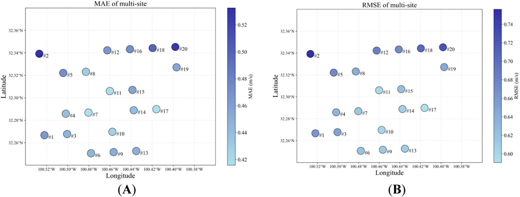
Figure 9. The prediction errors of multi-site under the MRGS-LSTM, the color of the ball indicates the MAE and RMSE values of the wind speed prediction results. (A) the MAE of multi-site. (B) the RMSE of multi-site.

Figure 10

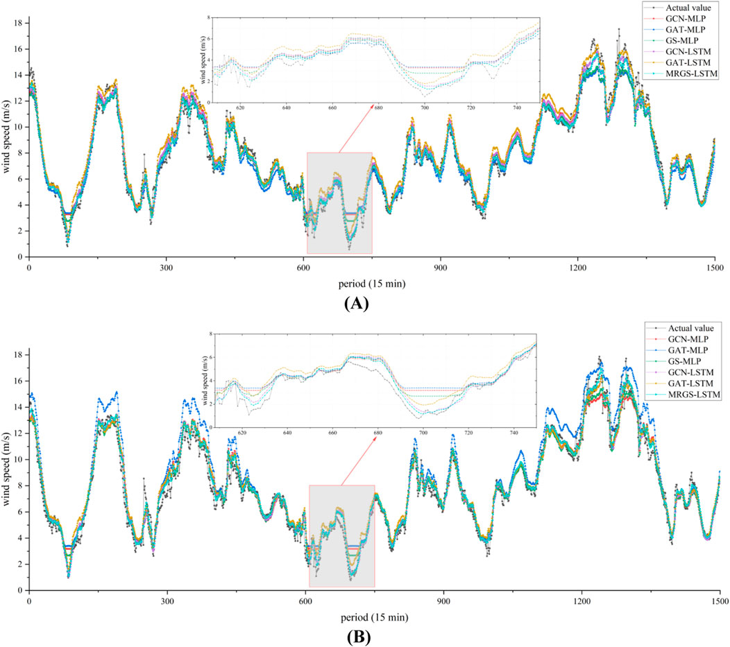
Figure 10. Prediction results of each prediction model. (A) Site #11. (B) Site #2.

5.4.4 Model training analysis

The training times of the different models are compared in Table 3. Our MRGS-LSTM model required the shortest training duration. Figure 11A shows the convergence curves of the prediction models on the training set. As the number of training epochs increases, these curves gradually decrease. This indicates that the models are constantly learning the known data, reducing the errors, and improving the performance. Figure 11B exhibits the convergence curves of the prediction models on the validation set of the dataset, demonstrating their effectiveness on unknown data. In both figures, it is evident that our MRGS-LSTM model surpasses the other models in terms of both the training and validation sets while exhibiting remarkable generalization ability without overfitting.

Table 3

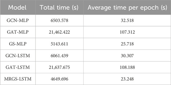
Table 3. Comparison of training times for different models.

Figure 11

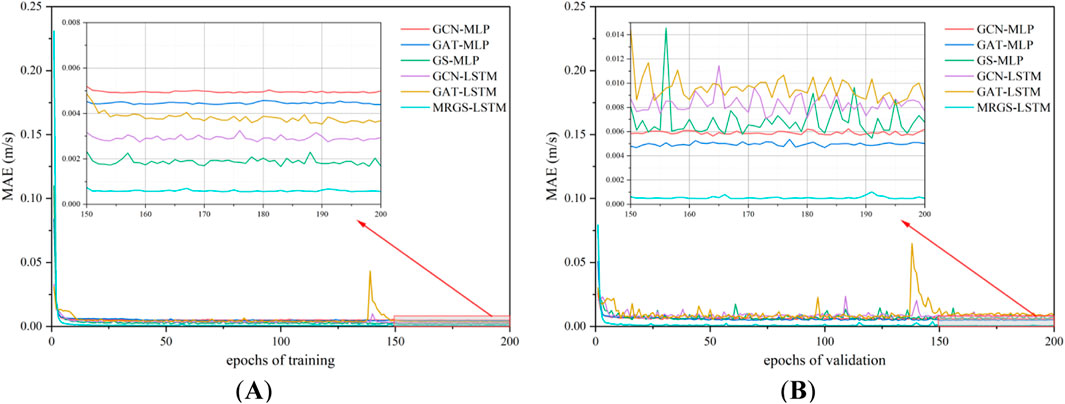
Figure 11. Convergence curves of the prediction models. (A) on the training set. (B) on the validation set.

6 Conclusion

This study proposes a novel multi-site wind speed prediction model, namely MRGS-LSTM, which leverages historical data on wind speed features from multi-site within the Roscoe Wind Farm in Texas, United States. By incorporating both spatial and temporal correlations, our proposed model enables accurate wind speed predictions at various locations.

Our approach effectively captures the topology of sites distribution within the wind farm and extracts spatio-temporal correlations from different features to enhance prediction accuracy. Firstly, we employ the mRMR-RF algorithm to obtain the fused feature with highly relevant and minimally redundant. Subsequently, based on spatial distance correlation and time series correlation between sites, we construct a weighted adjacency matrix that serves as input for the GraphSAGE network to update and aggregate wind speed features at each site, resulting in spatial feature vectors. Next, these spatial feature vectors are resampled by a sliding time window. The model utilizes LSTM memory cells to capture historical information from long time series data and obtain integrated spatio-temporal predictions. Finally, simulation experiments conduct with real historical data validate the effectiveness and accuracy of our proposed MRGS-LSTM model.

Although our model demonstrates promising results in wind speed prediction, further exploration is required regarding more precise integration of various spatial features for accurately predicting field-specific wind speeds. In future research endeavors, we plan to incorporate atmospheric factors such as air pressure and temperature as exogenous variables into the learning process to further enhance predictive capabilities.

Data availability statement

Publicly available datasets were analyzed in this study. This data can be found here: https://www.nrel.gov/grid/wind-toolkit.html, accessed on 20 February 2024.

Author contributions

YZ: Writing–review and editing, Writing–original draft, Visualization, Methodology, Investigation, Data curation, Conceptualization. XF: Writing–original draft, Methodology, Funding acquisition, Formal Analysis, Conceptualization.

Funding

The author(s) declare that financial support was received for the research, authorship, and/or publication of this article. This research was supported by the Key Research and Development Program of Hubei Province, China (Grant number 2021BAA193).

Conflict of interest

The authors declare that the research was conducted in the absence of any commercial or financial relationships that could be construed as a potential conflict of interest.

Publisher’s note

All claims expressed in this article are solely those of the authors and do not necessarily represent those of their affiliated organizations, or those of the publisher, the editors and the reviewers. Any product that may be evaluated in this article, or claim that may be made by its manufacturer, is not guaranteed or endorsed by the publisher.

References

Bai, W. W., Jin, M. X., Li, W. W., Zhao, J., Feng, B., Xie, T., et al. (2024). Multi-step prediction of wind power based on hybrid model with improved variational mode decomposition and sequence-to-sequence network. Processes 12 (1), 191. doi:10.3390/pr12010191

CrossRef Full Text | Google Scholar

Cadenas, E., Rivera, W., Campos-Amezcua, R., and Heard, C. (2016). Wind speed prediction using a univariate ARIMA model and a multivariate NARX model. Energies (Basel). 9 (2), 109. doi:10.3390/en9020109

CrossRef Full Text | Google Scholar

Chen, W. J., Qi, W. W., Li, Y., Zhang, J., Zhu, F., Xie, D., et al. (2021). Ultra-short-term wind power prediction based on bidirectional gated recurrent unit and transfer learning. Front. Energy Res. 9. doi:10.3389/fenrg.2021.808116

CrossRef Full Text | Google Scholar

Chen, Y., Zeng, Y., Luo, F., and Yuan, Z. M. (2016). A new algorithm to optimize maximal information coefficient. Plos One 11 (6), e0157567. doi:10.1371/journal.pone.0157567

PubMed Abstract | CrossRef Full Text | Google Scholar

Geng, X. L., Xu, L. Y., He, X. Y., and Yu, J. (2021). Graph optimization neural network with spatio-temporal correlation learning for multi-node offshore wind speed forecasting. Renew. Energy 180, 1014–1025. doi:10.1016/j.renene.2021.08.066

CrossRef Full Text | Google Scholar

Hamilton, W. L., Ying, R., and Leskovec, J. (2018). Inductive representation learning on large graphs. Arxiv. doi:10.48550/arXiv.1706.02216

CrossRef Full Text | Google Scholar

He, H. Y., Fu, F. Y., and Luo, D. S. (2022). Multiplex parallel GAT-ALSTM: a novel spatial-temporal learning model for multi-sites wind power collaborative forecasting. Front. Energy Res. 10. doi:10.3389/fenrg.2022.974682

CrossRef Full Text | Google Scholar

Hutchinson, M., and Zhao, F. (2023). Global wind report 2023. Rue de Commerce 31, 1000 Brussels, Belgium: GWEC Europe Office. Available at: https://gwec.net/wp-content/uploads/2023/04/GWEC-2023_interactive.pdf (Accessed February 10, 2024).

Google Scholar

Jager, D., and Andreas, A. (1996). NREL national wind technology center (NWTC): M2 tower; boulder, Colorado (data). Golden, CO, USA: National Renewable Energy Lab.

Google Scholar

Khodayar, M., and Wang, J. H. (2019). Spatio-temporal graph deep neural network for short-term wind speed forecasting. Ieee Trans. Sustain. Energy 10 (2), 670–681. doi:10.1109/tste.2018.2844102

CrossRef Full Text | Google Scholar

Khosravi, A., Koury, R. N. N., Machado, L., and Pabon, J. J. G. (2018). Prediction of wind speed and wind direction using artificial neural network, support vector regression and adaptive neuro-fuzzy inference system. Sustain. Energy Technol. Assessments 25, 146–160. doi:10.1016/j.seta.2018.01.001

CrossRef Full Text | Google Scholar

Kingma, D. P., and Ba, J. (2017). Adam: a method for stochastic optimization. Arxiv. doi:10.48550/arXiv.1412.6980

CrossRef Full Text | Google Scholar

Li, C. S., Tang, G., Xue, X. M., Saeed, A., and Hu, X. (2020). Short-term wind speed interval prediction based on ensemble GRU model. Ieee Trans. Sustain. Energy 11 (3), 1370–1380. doi:10.1109/tste.2019.2926147

CrossRef Full Text | Google Scholar

Li, H. (2022). Short-term wind power prediction via spatial temporal analysis and deep residual networks. Front. Energy Res. 10. doi:10.3389/fenrg.2022.920407

CrossRef Full Text | Google Scholar

Li, J. L., Song, Z. H., Wang, X. F., Wang, Y. R., and Jia, Y. Y. (2022). A novel offshore wind farm typhoon wind speed prediction model based on PSO–Bi-LSTM improved by VMD. Energy 251, 123848. doi:10.1016/j.energy.2022.123848

CrossRef Full Text | Google Scholar

Liu, H., Ma, H., and Hu, T. (2023a). Enhancing short-term wind speed forecasting using graph attention and frequency-enhanced mechanisms. Arxiv. arXiv:2305.11526. doi:10.48550/arXiv.2305.11526

CrossRef Full Text | Google Scholar

Liu, H., Mi, X. W., and Li, Y. F. (2018). Smart multi-step deep learning model for wind speed forecasting based on variational mode decomposition, singular spectrum analysis, LSTM network and ELM. Energy Convers. Manag. 159, 54–64. doi:10.1016/j.enconman.2018.01.010

CrossRef Full Text | Google Scholar

Liu, J. J., Yang, X. L., Zhang, D. H., Xu, P., Li, Z. L., and Hu, F. J. (2023b). Adaptive graph-learning convolutional network for multi-node offshore wind speed forecasting. J. Mar. Sci. Eng. 11 (4), 879. doi:10.3390/jmse11040879

CrossRef Full Text | Google Scholar

Liu, Z. Y., and Ware, T. (2022). Capturing spatial influence in wind prediction with a graph convolutional neural network. Front. Environ. Sci. 10. doi:10.3389/fenvs.2022.836050

CrossRef Full Text | Google Scholar

Nielson, J., and Bhaganagar, K. (2019). Using field data–based large eddy simulation to understand role of atmospheric stability on energy production of wind turbines. Wind Eng. 43, 625–638. doi:10.1177/0309524x18824540

CrossRef Full Text | Google Scholar

Nielson, J., Bhaganagar, K., Meka, R., and Alaeddini, A. (2020). Using atmospheric inputs for Artificial Neural Networks to improve wind turbine power prediction. Energy 190, 116273. doi:10.1016/j.energy.2019.116273

CrossRef Full Text | Google Scholar

Wang, F., Chen, P., Zhen, Z., Yin, R., Cao, C. M., Zhang, Y. G., et al. (2022). Dynamic spatio-temporal correlation and hierarchical directed graph structure based ultra-short-term wind farm cluster power forecasting method. Appl. Energy 323, 119579. doi:10.1016/j.apenergy.2022.119579

CrossRef Full Text | Google Scholar

Wang, Y. Q., and Gui, R. Z. (2022). A hybrid model for GRU ultra-short-term wind speed prediction based on tsfresh and sparse PCA. Energies 15 (20), 7567. doi:10.3390/en15207567

CrossRef Full Text | Google Scholar

Wang, Y. W., Sun, Y. Y., Li, Y. L., Feng, C., and Chen, P. (2023). Interval forecasting method of aggregate output for multiple wind farms using LSTM networks and time-varying regular vine copulas. Processes 11 (5), 1530. doi:10.3390/pr11051530

CrossRef Full Text | Google Scholar

Wu, Q. Y., Guan, F., Lv, C., and Huang, Y. Z. (2021). Ultra-short-term multi-step wind power forecasting based on CNN-LSTM. Iet Renew. Power Gener. 15 (5), 1019–1029. doi:10.1049/rpg2.12085

CrossRef Full Text | Google Scholar

Yu, B., Yin, H., and Zhu, Z. (2018). Spatio-temporal graph convolutional networks: a deep learning framework for traffic forecasting. Arxiv, 3634–3640. doi:10.24963/ijcai.2018/505

CrossRef Full Text | Google Scholar

Yu, E. B., Xu, G. J., Han, Y., and Li, Y. L. (2022). An efficient short-term wind speed prediction model based on cross-channel data integration and attention mechanisms. Energy 256, 124569. doi:10.1016/j.energy.2022.124569

CrossRef Full Text | Google Scholar

Zeng, W. L., Li, J., Quan, Z. B., and Lu, X. B. (2021). A deep graph-embedded LSTM neural network approach for airport delay prediction. J. Adv. Transp. 2021, 1–15. doi:10.1155/2021/6638130

CrossRef Full Text | Google Scholar

Zhang, Y. G., Pan, G. F., Chen, B., Han, J. Y., Zhao, Y., and Zhang, C. H. (2020). Short-term wind speed prediction model based on GA-ANN improved by VMD. Renew. Energy 156, 1373–1388. doi:10.1016/j.renene.2019.12.047

CrossRef Full Text | Google Scholar

Zhang, Z. D., Ye, L., Qin, H., Liu, Y. Q., Wang, C., Yu, X., et al. (2019). Wind speed prediction method using shared weight long short-term memory network and Gaussian process regression. Appl. Energy 247, 270–284. doi:10.1016/j.apenergy.2019.04.047

CrossRef Full Text | Google Scholar

Zhu, X. X., Liu, R. Z., Chen, Y., Gao, X. X., Wang, Y., and Xu, Z. X. (2021). Wind speed behaviors feather analysis and its utilization on wind speed prediction using 3D-CNN. Energy 236, 121523. doi:10.1016/j.energy.2021.121523

CrossRef Full Text | Google Scholar