 Yu Zhou
 Guillermo Narsilio3*
 Lu Aye
95% of researchers rate our articles as excellent or good
Learn more about the work of our research integrity team to safeguard the quality of each article we publish.
Find out more
ORIGINAL RESEARCH article
Front. Energy Res. , 12 June 2024
Sec. Sustainable Energy Systems
Volume 12 - 2024 | https://doi.org/10.3389/fenrg.2024.1423695
This article is part of the Research Topic Machine learning in Energy Conversion and Utilization View all articles
A Ground Coupled Heat Pump (GCHP) is a highly energy efficient heating, ventilation, and air conditioning (HVAC) system that utilises the ground as the heat source when heating and as the heat sink when cooling. This paper investigates GCHP systems with horizontal Ground Heat Exchangers (GHEs) in the rural industry, exemplifying the technology for poultry (chicken) sheds in Australia. This investigation aims to provide an Artificial Neural Network (ANN) model that can be used for GCHP design at various locations with different climates. To this extent, a Transient System Simulation Tool (TRNSYS) model for a typical horizontal GHE applied in a rural farm was first verified. Using this model, over 700,000 hourly performance data items were obtained, covering over 80 different yearly loading patterns under three different climate conditions. The simulated performance data was then used to train the ANN. As a result, the trained ANN can predict the performance of GCHP systems with identical (multiple) GHEs even under climatic conditions (and locations) that have not been specifically trained for. Unlike other works, the newly introduced ANN model is accurate even with limited types of input data, with high accuracy (less than 5% error in most cases tested). This ANN model is 100 times computationally faster than TRNSYS simulations and 10,000 times faster than finite element models.
• ANNs are used to predict the COP and GHE inlet and outlet temperatures.
• With only three types of input data, the error is less than 10% in most cases tested.
• The ANNs can be 100 times faster than TRNSYS and 10,000 times faster than FEM models.
• The ANNs models can be applied to similar cases for various locations.
Ground Coupled Heat Pump (GCHP) systems are renewable technologies and highly energy efficient Heating Ventilation and Air Conditioning (HVAC) systems that utilise the ground as a heat source or sink. The ground acts as the heat source when delivering heating and as a heat sink when providing space cooling. Recent years have witnessed an increase in applications of GCHP systems in the United States, Europe, Canada, China, Korea, and Australia (Omer, 2008; Yi et al., 2008; Self et al., 2013; Han and Yu, 2016; Lund and Boyd, 2016; Rees, 2016; Zhou et al., 2016; Lu et al., 2017). Ground Heat Exchangers (GHEs) are typically used to exchange heat with the ground. These are composed of high-density polyethylene (HDPE) pipes with a heat transfer (or carrier) fluid. GHEs can take numerous forms, including vertical boreholes, horizontal trenches, energy piles, energy retaining walls, and energy tunnels (Narsilio and Aye, 2018). Among them, vertical boreholes and horizontal trenches are the two most commonly utilised GHEs. While vertical boreholes can be installed under almost any ground and site conditions, horizontal trenches are typically used in suburban and rural areas at a depth of 1–2 m below the surface, as they usually require a large field of land to install them, but the capital cost is typically lower than that for drilling vertical boreholes. Since the heat exchangers are close to the ground surface, their thermal performances can be impacted by the daily and seasonal variation of the air temperature (Bidarmaghz et al., 2016a; Jensen-Page et al., 2018) and soil moisture content, the latter affecting the thermal conductivity of the ground (Demir et al., 2009; Beier and Holloway, 2015). A well-designed GCHP system with horizontal GHEs can typically operate at a coefficient of performance (COP) between 3 and 5 (Colangelo et al., 2005; Esen et al., 2007; Tarnawski et al., 2009; Johnston et al., 2011; Norway et al., 2012; Go et al., 2016; Zhou et al., 2018). The COP is defined as the ratio of heating (or cooling) supplied to the energy required to operate the GCHP. This means that for 3 to 5 kWh of energy removed/injected into the ground, only 1 kWh energy of electricity is consumed by the GCHP. Limitations of GCHP systems include high upfront construction costs mainly by the GHE installation (drilling/earthworks), as well as the embodied energy and associated greenhouse gas (GHG) emissions, odours and volatile compounds (e.g., ammonia gas, hydrogen sulphide, and mercaptans). However, these can be reduced by coupling GCHPs with other energy sources to form a hybrid system (Kjellsson et al., 2010; Eslami-Nejad and Bernier, 2011; Aditya et al., 2018). Previous studies indicated that a hybrid GCHP system is not only financially attractive but also helps to balance the thermal loads in the ground (Yi et al., 2008; Man et al., 2010; Kuzmic et al., 2016).
Current applications of GCHP systems span a wide range of end uses, including commercial office buildings, residential buildings, schools, hospitals, and underground metro stations (Omer, 2008; Yi et al., 2008; Self et al., 2013; Han and Yu, 2016; Lund and Boyd, 2016; Rees, 2016; Zhou et al., 2016; Lu et al., 2017). However, there is very limited focus on applying this relatively new technology in the rural industry, which could potentially be largely beneficial. For example, agriculture and its related processing industry in Australia, contributes to 12% of the national Gross Domestic Product (National Famer’s Federation, 2016). Within the Australian agriculture sector, this paper will primarily focus on the poultry industry, with over 600 million chickens raised yearly (Australian Bureau of Statistics, 2016). One of the major costs for poultry farmers and to the environment is the energy required to heat and cool large poultry breeding houses (estimated at A$80 million per year) (Zhou et al., 2017). The uniqueness of the heating and cooling load profiles of chicken broiler houses (a.k.a. sheds), together with the high risk of storing a high volume of combustible gas and the lack of access to (cheap) natural gas in rural areas where these houses are located, make the GCHP or shallow geothermal alternative a very attractive option. Its adoption can transform the poultry farming industry by significantly reducing energy consumption (and energy bills to farmers), GHG emissions, and chicken mortality (Choi et al., 2012), thus notably impacting the economics and environmental performance of the Australian poultry industry. As the rural industries’ unique loading patterns can be highly different from those of residential, commercial, and public buildings, detailed analyses are required to achieve an appropriate design of GCHP systems specifically for the rural industry.
In engineering practice, commercial software packages, including Ground Loop Design (GLD) and GLHEPRO (stands for ground loop heat exchanger) have been widely used in the analysis and design of GCHP systems (Q. Lu, 2018). Understanding the hourly performance of GCHP systems is important when detailed design or analysis are required. While hourly performance calculations are available for GCHP systems with vertical boreholes in both GLD and GLHE Pro, such a function is only just becoming available for GCHP systems with horizontal GHEs (only annual averages are outputted). One possible explanation for this limitation is that commercial software packages normally use simpler analytical models (for vertical GHEs) to provide quick calculations. While infinite line source, infinite cylindrical source, and finite line source models are popular in modelling vertical GHEs, these models cannot be directly used for horizontal GHEs. Hence, the applications of such similar sophisticated analytical methods in horizontal GHEs are currently limited and can be more difficult to be applied in commercial software (Zeng et al., 2002; Bandos et al., 2009; Philippe et al., 2009). This is mainly because the performance of the horizontal GHEs is highly affected by the configuration of the pipes and climate and geological conditions, which are difficult to cover in a generalised analytical model (Yuan et al., 2012).
When a detailed analysis is required, researchers have developed numerical simulation models to analyse GCHP systems with horizontal GHEs. As an example, Transient System Simulation Tool (TRNSYS) simulations are widely used in various types of building energy simulations (Magnier and Haghighat, 2010; Webb et al., 2018) and to predict the performance of GCHPs and GHEs (Safa et al., 2015). By using full implicit finite difference methods to solve three-dimensional meshed soil and GHE models, this approach can be implemented in the common practice of GCHPs with vertical or horizontal GHEs and can be modified to simulate complex GCHP applications such as GCHPs with dual sources or solar-assisted GCHPs (Trillat-Berdal et al., 2007; Chargui et al., 2012; Chargui and Sammouda, 2014; Weeratunge et al., 2018). Apart from TRNSYS, researchers have also developed other numerical simulation models and approaches, including Finite Element Modelling and Computational Fluid Dynamics (Tarnawski and Leong, 1993; Colangelo et al., 2005; Tarnawski et al., 2009; Wu et al., 2010; Norway et al., 2012; Chong et al., 2013; Go et al., 2016; Esen et al., 2017). Numerical simulation results can be in good agreement with the respective experiments and hence contribute to the optimum design of horizontal GHEs. However, current numerical simulation models, including TRNSYS simulations, are usually time-consuming, resource-demanding, and case-specific, which could limit their application in engineering practice.
Statistical and machine learning models represent potential approaches to accelerate simulations and ultimately design, with only a marginal compromise on accuracy.Recent years have witnessed substantial advancements in the field of artificial intelligence (AI)(Ahmad et al., 2021; Benzidia et al., 2021; Li and Li, 2023), especially in deep learning and natural language processing, showcasing notable progress across various academic and industrial spheres. In energy industry, attentions have been drawn to the application of machine learning technologies into energy production forecast, energy consumption forecast and energy consumption optimisation (Narciso and Martins, 2020). As summarised in Table 1, a wide range of applications of statistical and machine learning models have been adopted in energy systems, specifically Artificial Neural Networks (ANNs) (Kalogirou, 2000; Esen et al., 2008b; Esen and Inalli, 2009; Cai et al., 2014; Afram et al., 2017; Guo et al., 2018; Makasis et al., 2018; Wang et al., 2018). Well-designed and properly trained ANNs can provide reasonably accurate results almost instantly when applied in GCHP systems. As shown in Table 1, different types of neural networks and machine learning tools have been tested on GCHP systems, including Feedforward Neuron Networks (FFNN), Adaptive Neuro Fuzzy Inference Systems (ANFIS), Nonlinear Autoregressive Exogenous models (NARX), and Extreme Learning Machines. While FFNN has been identified as the best-performing tool for the performance prediction of GCHPs, NARX is very good in time-series predictions, including prediction of temperature and load series. However, there is very limited research currently available regarding the application of ANNs in GCHP systems with horizontal GHEs, with none found that consider rural industries’ unique loading conditions. Moreover, current ANN applications in GCHP systems are mostly based on case-specific studies, meaning they cannot be generalised and applied to different cases than those for which they were created.
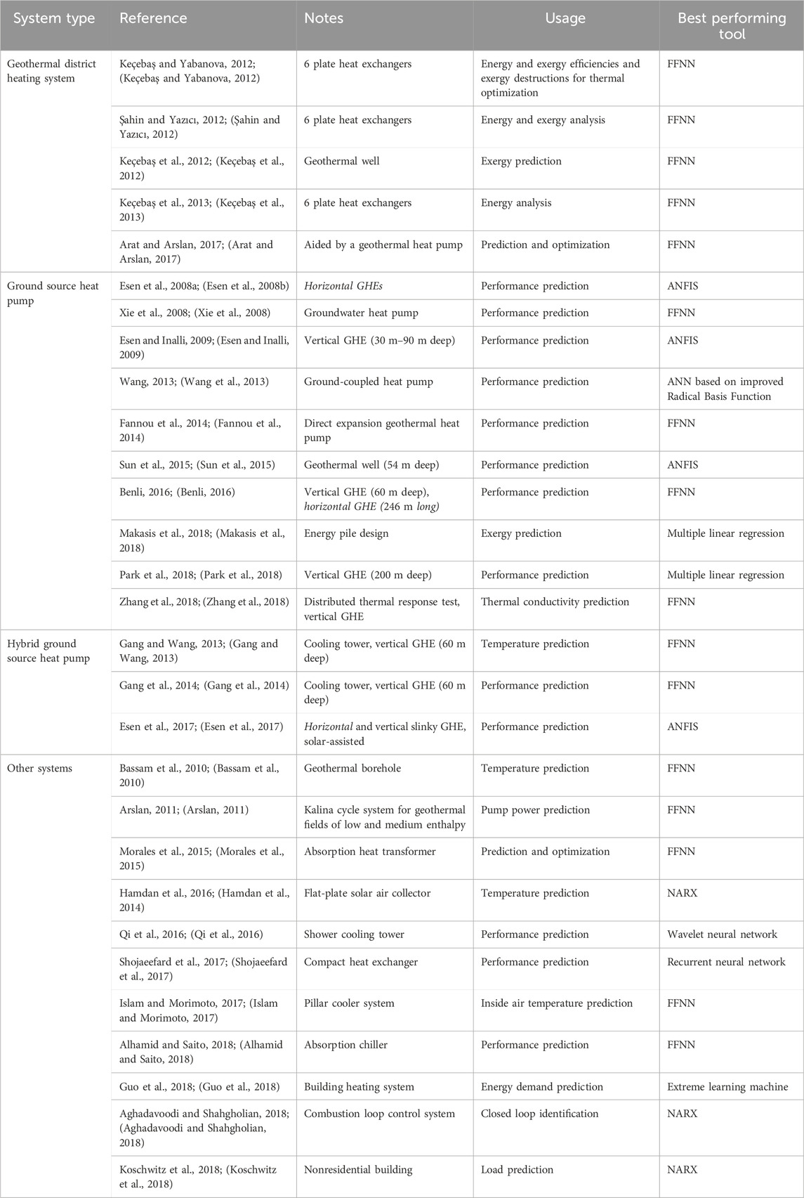
Table 1. Summary of published research regarding ANN for GCHP systems.
Within the handful of pioneering ANN studies dealing with horizontal GHEs currently available in the literature, Esen et al. and Benli’s ANN models are the only ones that can predict the COP of water-to-air GCHPs with horizontal GHEs using pre-processed input data (Esen et al., 2008a; Benli, 2016; Esen et al., 2017). Their results show the ANN can predict the COP well when enough input data are given. Their methodologies require three to five types of input data, including, at a minimum, the inlet air, outlet air, and ground temperatures. In their most recent work, Esen and coworkers (Esen et al., 2017) utilised ground temperatures at seven different depths, inlet air, outlet air, ambient air, tank water, inlet water, and outlet temperatures as inputs to the predictive model. However, these input data cannot be acquired easily, and more importantly, it would be arguably simpler and faster to find the COP via the heat pump specifications if these data are accessible. Moreover, the input data required by current ANNs can typically be part of the output needed for GCHP system design, making these works, while insightful, of limited use in practice. Last, the ANNs found in the literature have limited applicability for broader utilisation, as their validity is mostly shown for the case with which they were studied/trained.
This study aims to provide an ANN methodology that can predict and tremendously accelerate the design of GCHPs with horizontal GHEs (using numerical simulations) under loading conditions in rural industries and with limited input data types. A Transient System Simulation Tool (TRNSYS) model for a typical horizontal GHE field arrangement (details in Section 3.1) is developed and verified, and the resulting simulated performance data are used to train the ANNs. The trained ANNs are then used to predict the performance of GCHPs with identical GHEs but varying the number of GHEs in other locations that are not in the training dataset to showcase its applicability for broader utilisation.
As mentioned in the Introduction, since the rural industries’ thermal loading patterns can be substantially different from those of commercial and residential building applications, the GCHP design requires careful and detailed analysis. As an example of these unique loading patterns and to exemplify the study for temperate climate regions, in this investigation, a chicken shed building in Peats Ridge, New South Wales (NSW), Australia, is adopted. The schematic of the typical test broiler house (or shed) with a hybrid GCHP system is depicted in Figure 1. The system consists of several identical single-speed GCHPs with a 20 kW heating capacity are utilised to provide the required thermal energy. Each heat pump has a fixed ground heat exchanger field configuration formed by four horizontal trenches. The length for each trench is 75 m, rendering a pipe length of about 300 m per trench. The details of the system are further illustrated in Section 3.1.
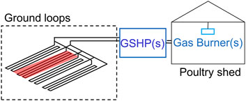
Figure 1. Diagram of hybrid geothermal systems for poultry shed. Each trench is 75 m long and contains 300 m of HDPE pipe (highlighted in red).
A building energy simulation model was developed for the shed using a transient system simulation software TRNSYS 18, which simulates the heating and cooling loads for the shed. The location and parameters used for the simulation are summarised in Table 2. For this study, the shed is used for six chicken-raising cycles per year (from chicks to chicken for meat) as per typical broiler house operation, with the first raising cycle for the chickens assumed to start on the 1st of January. Each cycle is assumed to last 7 weeks, with a 2-week break time between batches (Zhou et al., 2018).
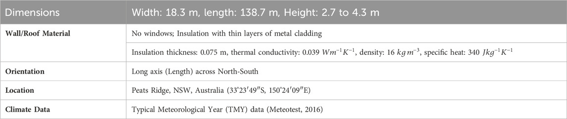
Table 2. Typical broiler house dimensions and temperate climate case-study location.
A previous study identified that although there is a high cooling demand, cooling can be economically provided via evaporative coolers (Zhou et al., 2017). Hence, the primary focus of this work is to provide heating via a hybrid geothermal-gas system. Figure 2 shows the simulated heating power demand of the shed based on the building energy consumption model developed. It was estimated that the annual heating energy of the shed is 58,477 kWh with a peak heating power demand of 208 kW. During each heating cycle, the heating demand is usually at its maximum at the start of each cycle when the least metabolic heat is generated by chickens and, the required indoor temperature is at its maximum (typically 31°C). The heating demand decreases later in each cycle owing to the increase in metabolic heat generated by chickens and the lower indoor temperature requirement corresponding to the age of the cycle (typically to a minimum of 19°C within 21 days of the start of the cycle).
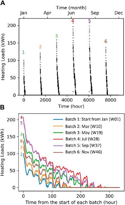
Figure 2. Hourly heating demand of chicken shed: (A) yearly loading pattern showing six batches (B) detail of these six heating cycles over 1 year, starting week 1, 10, 19, 28, 37, and 46 respectively.
To provide the heating load demand for the building, a hybrid GCHP system with horizontal GHEs is employed. As the initial installation cost of GHEs can be relatively high, the chosen hybrid geothermal-gas system help to reduce the capital cost while maintaining most benefits of the geothermal (GCHP) technology. In this hybrid system, the heating is delivered by several identical GCHPs connected in parallel to a main header pipe. Each GCHP is coupled to several GHEs connected in parallel as well. The LPG gas burners installed in the shed can top up the heating when needed. A “shave factor” S is used to describe the capacity portion of the GCHP in the hybrid system. It is defined as the ratio of the installed capacity of the GCHP of the system to the peak heating demand of the load to be satisfied by the hybrid system (Alavy et al., 2013; Mikhaylova et al., 2016):
In this study, a 0% shave factor represents a full gas system and 100%, a full GCHP system. A shave factor of 40% in this GCHP-gas hybrid system of 208 kW peak load means that the installed capacity of the GCHPs is
To further investigate this hybrid system, other locations across Australia under different climate conditions are analysed following similar approaches. These places are significant due to their prominence in the poultry industry. Together with the one mentioned above, these three locations represent conditions in Queensland (QLD), New South Wales (NSW), and Victoria (VIC) (Figure 3). The three states analysed in this study are known for housing a significant portion of Australia’s poultry farms and production facilities, accounting for 74.4% of Australia’s overall broiler production with different climate conditions (Australian Chicken Meat Federation ACMF Inc, 2016; The Bureau of Meteorology & CSIRO, 2016). The peak heating loads and annual energy demand are 228 kW and 73,456 kWh for Mornington Peninsula, VIC, and 164 kW and 34,149 kWh for sunshine Coast, QLD.
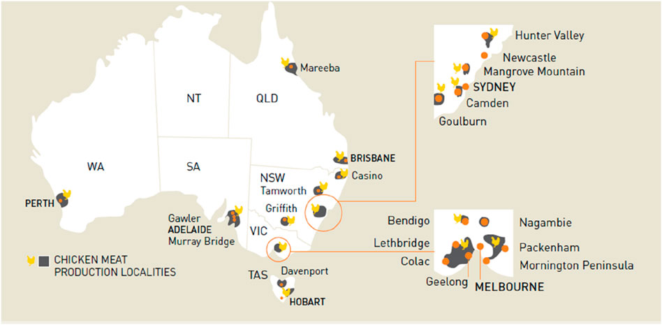
Figure 3. Chicken industry profile in Australia (Australian Chicken Meat Federation ACMF Inc, 2016).
The latest average annual temperatures (maximum, minimum, and average) are summarised in Table 3. For the building side, all other factors besides the climatic conditions associated with the different locations, such as the shed envelope, orientation, and ventilation conditions, are kept constant in this study to ensure a representative comparison between them.

Table 3. Simulation locations and key climate data (DOM, 2018).
Besides the three discussed locations for training (and testing), three additional test cases, one in Warracknabeal (Victoria), one in Murray Ridge (South Australia), and an extra one in Gaborone (Botswana, annual average temperature 20.6°C) were adopted to further check the accuracy of the ANN model results and flexibility to accommodate different site conditions. The data relating to these test cases are not part of the training dataset (Table 3) and can therefore be used to evaluate the accuracy of the prediction ANN model after it has been trained.
In this study, a TRNSYS simulation model is developed for the poultry industry and is utilised to simulate over 700,000 hourly performance data items covering over 80 different yearly thermal loading patterns (by varying the shave factors) under three different climate conditions. The simulation data from the completed TRNSYS models are then used to train the ANNs.
To generate data to train the ANN, a typical poultry shed in Australia equipped with a hybrid GCHP system to provide the required heating is utilised (Zhou et al., 2018). As mentioned in Section 2, the hybrid system comprises several identical GCHPs with horizontal GHEs and gas burners. The sizing and configuration of the GCHPs and the gas burners within the hybrid system vary based on the thermal demand and the different shave factors determining it. The TRNSYS model is used to evaluate the hourly performance of the GCHPs for each of these cases of different thermal load and configurations. A Typical Meteorological Year (TMY) dataset was used as the boundary condition of the soil surface. The soil is meshed three-dimensionally, and a fully implicit finite difference method is utilised in the modelling. For all the models, a sandy clay soil is assumed with an average thermal conductivity of about 2
In the modelled systems, several identical single-speed GCHPs with a 20 kW heating capacity are utilised to provide the required thermal energy. Each heat pump has a fixed ground heat exchanger field configuration formed by four horizontal trenches. Each trench is dug at a depth of 1.5 m below the ground surface, and there are four straight pipes in each trench with a 300-mm separation between each pipe. The length for each trench is 75 m, rendering a pipe length of about 300 m per trench. As an example of an overall system, to provide 208 kW of peak heating in total at a shave factor of 38% (therefore requiring 80 kW), four 20 kW heat pumps are installed, each with its own ground heat exchanger field in four trenches (i.e., 16 trenches in total). For simplicity, the thermal conductivity of the soil was assumed the same for different locations; however, the ground temperature reflects that of each site (see Table 3). It is also assumed that all trenches are placed sufficiently apart from each other to minimise any thermal interference between them.
The operation of the heat pumps is controlled by the hourly loading demand. When the operation of a new heat pump is required, the one with the lowest accumulated hours of operation will start. For example, in the 208 kW total capacity case above (with 80 kW provided by the GCHPs, i.e., S = 38%), when the loads increase from 19 kW to 35 kW, the operation of a second 20 kW heat pump is required. At this time, the system will compare the accumulated hours of operation from the three heat pumps that are not operating and turn on the one with the lowest accumulated hours of operation. In this way, the loads can be relatively evenly divided amongst all the heat pumps throughout the life of the system. For heating demands over 80 kW, all four GCHPs will be in operation, and the gas burners will provide the balance of the required load.
Figure 4 shows the configuration of the TRNSYS model for each GCHP. This model simulates one water-to-water GCHP (Type 927) with a short-distance (5 m) buried head pipe (Type 951) and a horizontal ground heat exchanger (Type 997) composed of the four 75-m long trenches (recall Figure 1). In the TRNSYS simulation, horizontal ground heat exchanger are governed by a fully 3-D rectangular conduction model of the ground, which considers the insulation and the impact of energy storage in the ground.The thermal loads generated from TRNSYS are imported to the water heat exchanger (Type 682) to simulate the loading from the building. A control unit (Type 1502) together with the Typical Meteorological Year TMY weather data (Type 15–6) generated from Meteonorm, a widely used weather analysis software package, complete the TRNSYS model of the smallest GCHP component (20 kW) of the hybrid system. Further details of the physics, including governing pheonomena can be found in TRNSYS manual, availble online on TRNSYS website support page.
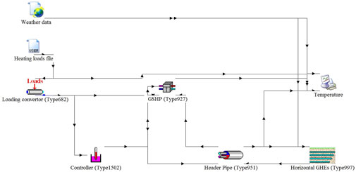
Figure 4. Schematic of the TRNSYS model.
In this TRNSYS model, only one heat pump is simulated with a fixed load input (heating loads are inputted from outside files with data generated). However, for one particular scenario, each of the GCHPs involved receives a unique loading pattern based on the system’s operation. For example, when the shave factor is 100% in the NSW training case, 208 kW peak loads need to be covered by 11 GCHPs (of 20 kW capacity each).
Accordingly, 80 different loading patterns for the GCHP are generated as inputs, depending on when each heat pump needs to be turned on or off. Therefore, considering that simulations have been conducted for different shave factors and locations and for each shaved factor multiple GCHPs might be needed with different loading patterns, over 30 simulations are considered for the training case in NSW and 25 for each of the training cases in VIC and QLD. Therefore more than 80 simulations (each with unique loading patterns/conditions) and over 700,000 h of simulation data are generated and will be used to train the ANNs, as explained in Section 4.
Following the discussion on the methodology and data mentioned in previous section, this section presents the simulation results from TRNSYS. These results are used in the prediction model both as inputs as well as outputs (to train the prediction model as well as compare the results to evaluate its accuracy). These include a loading pattern as an example for the inputs and the simulated hourly COP and inlet and outlet temperatures of the GHEs as examples for the outputs.
As an example, Figure 5 shows one of the 80 loading patterns used for the simulation of one GCHP (connected to a set of four trenches, the GHE field) in a hybrid GCHP-gas system in NSW with a shave factor of 25% (or 52 kW of GCHP capacity for a total peak demand of the entire system at 208 kW; see Section 2).
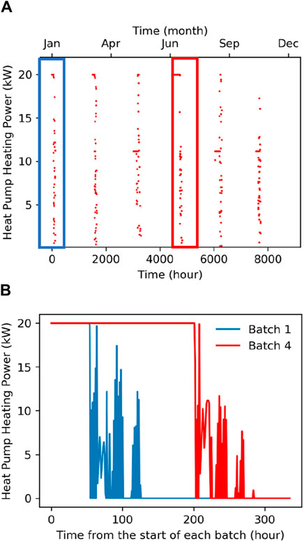
Figure 5. Hourly heating load pattern example for 20 kW capacity GCHP: (A) overall yearly load, and (B) detail of lowest (Batch 1, January, in blue) and highest (Batch 4, July, in red) GCHP run fraction batch loads.
Figure 6 shows the results of the simulation based on the loading pattern in Figure 5 and weather in Peats Ridge, NSW. As seen, the GHE inlet and outlet temperatures (or LWT and EWT1, respectively) vary with the loading and seasons as expected. The maximum is about 20.3°C, and the minimum is about 5.8°C. When there is loading, the GHE outlet temperature is higher than the GHE inlet temperature by 1°C–2°C. The resulting
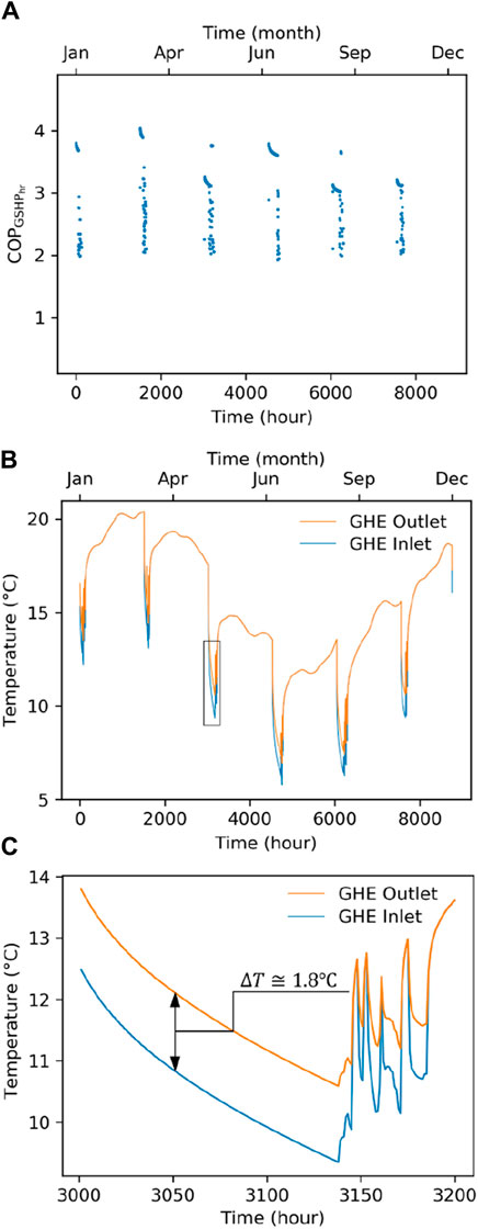
Figure 6. Typical TRNSYS simulation results: (A) hourly COP of an individual heat pump
The simulations used within this work model 1 year of operation of the system using the TMY data. In order, however, to test that the tools and insights from this work are also representative of a long-term performance analysis, a longer 10-year simulation was also undertaken using annually repeating TMY data. The results show that the
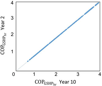
Figure 7. Correlations between a 2nd year and 10th year
The next section presents the ANN models (which use the above results from TRNSYS for training, validation, and testing) and their simulation results, including:
An artificial neural network (ANN) is a mathematical approach that simulates a network of artificial neurons to mimic the human brain. With a well-trained ANN, a computer can be taught to solve problems, including generalisation, classification, forecasting, and even decision-making [83]. In this study, two ANN models are developed and implemented using MATLAB: 1) a feedforward artificial neural network (FFNN) is used to predict the performance of the GCHPs in terms of
The FFNN statistical model, also referred to as a multilayer perceptron (MLP) or simply artificial neural network (ANN) in some studies, is by far the most popular machine learning tool used in energy-related fields. It is versatile and may model complex systems with great accuracy, including but not limited to geothermal district heating systems (Keçebaş and Yabanova, 2012; Keçebaş et al., 2013; Arat and Arslan, 2017), geothermal walls (Bassam et al., 2010), and GCHP or hybrid GCHP systems (Benli, 2016). In this work, an FFNN is developed to predict the COP of the GCHPs (
Although various types of datasets can be set as feature variables, such as the inlet air, outlet air (on the building side of the GCHP), ground, and the inlet and outlet GHE water temperatures (on the ground side of the GCHP), the complexity of acquiring them may make the FFNN not feasible in engineering practice. Instead, in this study, the input layer comprises three neurons which represent the three easy-to-acquire influencing factors for the performance of the GCHPs: the hourly loads (which are typically known), the hourly accumulated loads, and the moving average monthly outdoor temperature [which can be readily obtained from the Typical Meteorological Year (TMY, Meteonorm) when designing a system or via weather stations or sensors when optimising scheduling of the system dynamically].
Hourly heating loads: The simulated hourly heating loads that will be delivered by the GCHPs to the building. As explained in Section 2 and Section 3, these hourly loads between GCHPs vary based on the control strategy, the shave factor adopted, and the operating conditions of each GCHP.
Adjusted accumulated heating loads: Since the continuing heating operation of the heat pumps can impact the performance, the hourly loads, showing the demand at a specific point in time, are not sufficient to fully capture the problem and train the network. Thus, the accumulated thermal loads are introduced to represent the short-term effects of heating the ground and its recovery. In this study, this value is estimated based on the hourly heating loads and the ground conductive heat flux (Carslaw and Jaeger, 1959; Wang and Bras, 1999; Larwa, 2018). As the GHE pipes are buried 1.5 m deep, the conductive heat flux is the primary heat flux at this depth and can range from 6 to 14 W/m2 depending on the moisture content of the soil (Larwa, 2018). In this study, the ground heat flux fg is assumed to be 10 W/m2. Since the area of the GHE trench field in this study is about 1,500 m2 (four trenches per GCHP), the estimated heat flux is 15,000 W.
where
Outdoor ambient air temperature: This input represents the variation introduced to the performance of the heat pumps owing to the seasonality. The air temperature can be used with some delay to represent the ground temperature (and therefore the neutral ground condition) (Kusuda and Achenbach, 1965; Baggs, 1983). In this work, a moving average monthly outdoor temperature is introduced to simply but effectively represent the effects of the daily and seasonal variation. By applying a 2-week delay, the moving average monthly outdoor temperature showed a reasonably good correlation to the TRNSYS simulated ground temperature at 1.5 m deep.
The hidden layer is used as an intermediary between the input and output to enable the predictions and transformation of the input to output. In this study, the hidden layer comprises 1 layer of 10 neurons of a feedforward network. The transfer functions in the hidden layer are sigmoid functions, which are most commonly utilised throughout the literature and make it possible to solve nonlinear problems. As shown in Section 4.4, 10 is found to be the optimum number for the neurons in the hidden layer.
The aim of the FFNN is to predict the performance of each GCHP. In this case, the output layer has only one neuron, which carries the hourly COP of the modelled GCHP (
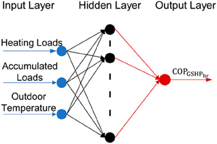
Figure 8. Structure of a FFNN model to calculate the COP of 20 kW GCHP.
The NARX architecture is well-suited for circumstances with the presence of long-term dependencies, outperforming certain variations of recurrent neural networks (Lin et al., 1996), which can be advantageous in many time-series prediction problems. As a result, NARX networks work well in prediction problems in which temporal patterns may be present and negatively influence some of the other models.
The initial input variables are the same as the input variables in the NARX for GCHPs as in the FFNN section. To establish a continuous time series analysis, the output inlet and outlet temperatures of the model from the previous time step serves as the new input for the current time step.
The hidden layer comprises 1 layer of 10 neurons of a NARX network. As the base architecture of the NARX network is a feedforward network, this layer also follows the same reasoning as that of the FFNN model of Section 5.1, also with 10 neurons and sigmoid transfer functions.
The aim of the NARX network is to predict the inlet and outlet temperatures of the GHEs. In this case, the output layer has two neurons representing the hourly inlet and outlet temperatures of the GHEs (Figure 9). The values of these parameters are used in each following iteration of the NARX calculations for the time series (i.e., the temperatures for time t are used to compute the temperatures for time t + 1). These results are important when evaluating the design length of GHEs and can directly impact the COP of GCHPs.
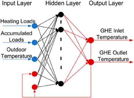
Figure 9. Structure of the NARX model for GHE.
There are different learning algorithms to train and test the FFNN and NARX, including Levenberg-Marquardt and BFGS Quasi-Newton (Martinez and Martinez, 2015). In this study, the Levenberg-Marquardt method is selected owing to its popularity and high speed. The simulated data from the TRNSYS simulation are used to train and test both the FFNN and NARX models. As explained in Section 3, there are different thermal loading conditions for heat pumps under different shave factors and climate conditions. This covers in total over 80 different operational conditions across three locations in Australia (Table 3). The trained FFNN and NARX models are then tested by several operational conditions in other three locations (Table 3). The Root Mean Square Error (RMSE) and Absolute Square Error (MAE) are used to quantify the performance of these models.
Based on the models and algorithm mentioned above, this section presents the prediction results from the two ANN networks. The first FFNN model predicts the
This section presents the results comparing the FFNN predictions with the respective time-consuming TRNSYS simulations. As an example, Figure 10 shows this comparison for the test case in VIC and 100% shave factor (Case 4 in Table 4). The results from the FFNN prediction of the
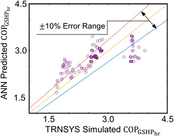
Figure 10. Hourly COP from TRNSYS simulation vs. ANN prediction (100% shave factor test case in VIC).
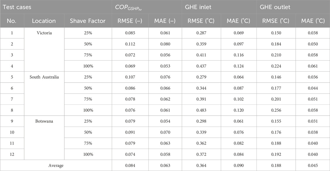
Table 4. RMSE and MAE for test cases.
A more holistic view of the testing results considering 11 other cases (and including both FFNN and NARX results discussed later) can be seen in Table 4, showing the RMSE and Mean Absolute Square Error (MAE). The results are reasonably consistent in all the test cases. Moreover, Figure 11A shows the
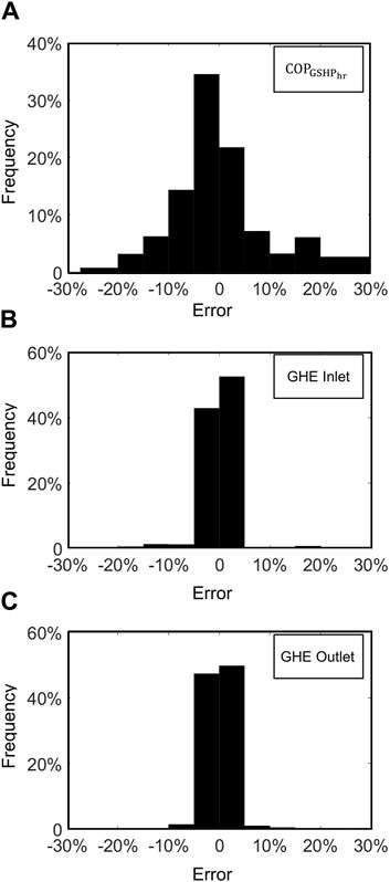
Figure 11. Error distribution for all testing cases: (A)
All the results presented here are based on having 10 neurons in the hidden layer. Figure 12 shows the RMSE with the number of neurons in the hidden layer for all cases, showing that the optimum number of neurons that minimises the error is about 10.
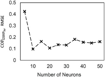
Figure 12. RMSE for different numbers of neurons in hidden layer.
The results for the temperature predictions using NARX are overall very promising. As shown in Figure 13A (Case 5, with a 25% shave factor test case in SA), the prediction results for the GHE inlet temperature from the NARX models compares well with the simulation results from the TRNSYS simulations for the test farm in VIC. The results are in a reasonable agreement with the TRNSYS simulation, with about 95% of the data having an error of less than ± 5%. Moreover, when considering all the testing cases, 98% of the results have an error of less than 1°C, and 96.3% of the data points fall into the ±5% error range as depicted in Figure 11B, which shows the GHE inlet error distribution of all testing cases. The results also show a reasonable consistency in all the test cases, with a slightly lower error when the shave factor is low (Table 4).
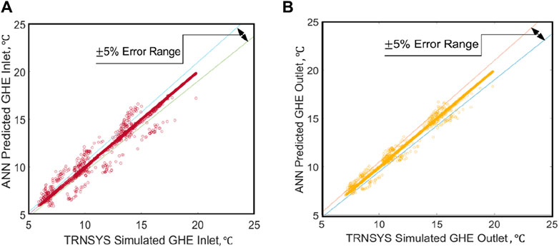
Figure 13. Hourly GHE temperatures from TRNSYS simulation and ANN: (A) GHE inlet, (B) GHE outlet.
Figure 13B presents the analogous results for the GHE outlet temperature (Case 5, with a 25% shave factor test case in SA), showing that the prediction results of the from the NARX prediction compare very well with those obtained via the TRNSYS simulation. Approximately 99% of the results have an error of less than 1°C, and approximately 98% of the data points fall into the ± 5% error range. When considering the overall analysis and all other testing cases (Table 4), the results also show reasonable consistency, with a slightly lower error when the shave factor is low. Figure 11C shows the GHE outlet error distribution of all 12 testing cases.
Following the results presented above, this section further discusses the key findings, limitations, and highlights of this study.
Our approach champions the principle of Occam’s Razor, which advocates for using the simplest tool to solve complex problems. In this context, our expertise in mechanical and geotechnical engineering has led us to employ the NARX model with inputs that physically linked with the phenomena we are investigating, which has proven to yield accurate predictions.
The two ANN prediction models can obtain the COP (FFNN model) and the GHE inlet and outlet temperatures (NARX model) of hybrid GCHP systems with horizontal GHEs in rural industries. The models only require three input parameters and have been shown to perform reasonably well.While the architecture of our Artificial Neural Network (ANN) model is simple, it is the training with dataset that physically linked with the phenomena of the NARX model within this framework that sets our approach apart. By leveraging our expert knowledge and experience, we have designed a straightforward set of inputs that effectively captures the intricacies of GCHP performance in various locations. This ultimately enhances the capability of our approach to accurately predict GCHP performance in these settings.
Looking at the results closely, an interesting observation is that there seems to be a trend for the FFNN to underestimate the COP during the peak of winter when the heat pump is under full loading. This is possibly caused by the limited sets of feature variables. As the performance of GCHPs is determined by the inlet and outlet temperatures of the building side and the ground side, the feature variables may not contain enough information for a perfect prediction. If the inlet and outlet temperatures are used as inputs, the prediction of the performance of the GCHPs could be improved. However, this will make the FFNN less practical as the GHE inlet and outlet temperatures are normally difficult to obtain.
Another highlight of this work is that the ANNs have been tested with a broad selection of cases. Trained with the simulated dataset in three locations from TRNSYS, the ANNs can predict the performance of the GCHPs and the horizontal GHEs in other untrained locations reasonably well. This suggests a generalisation ability for the ANN model that can potentially be widely used in prediction, optimisation, and control problems. Even though one limitation is that the ANN is only for a 75-m-long trench with 300 m of pipes, it can still benefit the designers as a comparison metric or by comprising the loops for one heat pump by a combination of several 75-m trenches. Since hourly simulation data for horizontal GHES are not available in any commercial software at this stage, the results from this ANN can provide the designers with some confidence.
Finally, a comparison between the computational time of the ANN, TRNSYS simulation and finite element simulation are shown in Table 5. This table summarised the computational time of 1-year simulation (time step in 1 hour) for the inlet and outlet temperature of horizontal GHEs. A typical personal computer was used to run these simulations (Windows 7, i7-5600U CPU, 16 GB of RAM), for a fair comparison and to showcase the methodology’s accessibility. The ANN and TRNSYS model were as described previously in this paper.
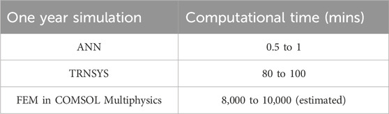
Table 5. Computational time comparison for ANN, TRNSYS, and FEM simulation.
The Finite Element Modelling (FEM) model was developed in COMSOL Multiphysics (Bidarmaghz, 2015) and is based on the coupling of the governing equations of heat transfer (energy balance) and fluid flow (momentum and continuity) similarly as in (Bidarmaghz et al., 2016b; Jensen-Page et al., 2018) but with horizontal GHEs. The heat transfer mechanism in this model is primarily the heat conduction in the soil, the pipe walls, and partly in the carrying fluid and the heat convection in the carrying fluid. The FEM model is solved with similar boundary conditions as the TRNSYS model (i.e., adiabatic conditions on four sides of the field, The outdoor temperature on the top and the undisturbed ground temperature at the bottom). The details of the FEM model can be found in the recent research (Zhou et al., 2021).
In terms of a direct comparison with other approaches, we must emphasize the limitations of commercial software in predicting hourly temperature for horizontal GHEs. Additionally, widely-used simulation software such as COMSOL and TRNSYS require significantly longer time (up to 10,000 times more) and input-intensive processes, making them less practical for predicting GCHP performance.
We firmly believe that our approach, with its successful implementation of the NARX model and focused inputs, offers a more capable solution for accurately predicting GCHP performance in various locations.
Even though the
This investigation proposed a NARX model that can predict the inlet and outlet temperatures, and from a statistical perspective, the results can be considered reasonably good as 99% of the results have an error less than 1°C. However, since the temperature difference (ΔΤ) between inlet and outlet is an important parameter for the performance of the system and ΔT for these systems is typically in the range of 1°C–5°C, errors from the NARX predictions can be propagated in the ΔΤ calculations and be significant. However, it is worth noting that the error of 1°C of the NARX predictions for the inlet temperature and outlet temperature of GHEs does not necessarily represent a high error in the temperature difference, as both inlet and outlet temperatures can be equally over- or under-predicted.
To further enhance the applicability and validity of using machine learning approaches with horizontal geothermal systems, future work aims to incorporate more complex (deep) neural network architectures as well as other predictive models. This work focused on relatively simple ANN architectures, as more complex models can be more time-demanding, harder to adopt by engineers, scientists, and practitioners, and often too specific for a wider adoption. However, these models can also significantly increase accuracy and therefore a comprehensive comparison can be beneficial. Another potential avenue for expansion is implementing on-line training, which can be relevant in a context of a system controller.
Additionally, future studies can investigate the impact of temperature difference on the accuracy of the predictions. This will help to provide a more comprehensive understanding of the analysis of GCHP and GHE systems. Furthermore, studies can be extended with consideration of thermal conductivity, initial ground temperature as well as trench distance, as these parameters directly affect the performance of the GHEs.
This article presented an investigation of the applicability of a hybrid GCHP system with horizontal GHEs in the poultry industry with unique heating dominant thermal load requirements. A TRNSYS simulation model for the performance of the system was developed and utilised to generate data for the ANN model. Statistical machine learning approaches (Artificial Neural Networks ANN) were adopted and fine-tuned to accelerate computational times.
In horizontal GCHP systems, no annual cumulative effects were observed since the natural thermal recharge of the horizontal GHEs is sufficient to restore the ground to its initial state, even under extremely imbalanced load conditions. This allows for the simulation of only 1 year of operation to provide insight into long-term system performance. It was also observed that there is a decreasing trend in the performance of the GCHP system when the shave factor is increasing. This may be counterintuitive, but it has been proven to be the effect of the partial load on the heat pump. This observation also suggests that, when designing a hybrid geothermal system, the sizing of the GCHP needs to be analysed in detail.
Since hourly simulation data for horizontal GHEs are not available in commercial software at this stage and numerical approaches, including TRNSYS simulations or FEM, can be computationally expensive, two different ANNs for the prediction of the performance of GCHPs and horizontal GHEs were developed and introduced. Trained with the simulated dataset from the TRNSYS results for three different locations, the ANNs can predict the performance of the GCHPs in other untrained (previously unseen) locations reasonably well (less than 5% error in COP for most cases) and the performance of horizontal GHEs reasonably well (less than 3% error in GHE water temperature error for most cases). This suggests that the ANN models developed here can potentially be widely used in prediction, optimisation, and control problems for similar sites and conditions.
A computational time comparison of the ANN predictions and TRNSYS and FEM simulations was presented. The results showed ANNs can predict reasonably well and 100 times faster than TRNSYS simulations and approximately 10,000 times faster than FEM simulations. Overall, it is believed that this work will contribute to the wider application of ANNs in GCHP systems.
The raw data supporting the conclusion of this article will be made available by the authors, without undue reservation.
YZ: Data curation, Investigation, Methodology, Validation, Visualization, Writing–original draft, Writing–review and editing. GN: Funding acquisition, Project administration, Supervision, Writing–original draft, Writing–review and editing. NM: Methodology, Writing–original draft, Writing–review and editing. KS: Methodology, Writing–original draft, Writing–review and editing. PC: Funding acquisition, Writing–original draft, Writing–review and editing. LA: Methodology, Project administration, Software, Supervision, Writing–original draft, Writing–review and editing.
The author(s) declare that financial support was received for the research, authorship, and/or publication of this article. The authors would like to thank the Australian Research Council for funding Linkage Projects LP160100070 and FT140100227, and follow up ARENA Grant 2021-ARP009.
The authors would also like to acknowledge the effort that Ms. Yuqi Kuai made during her final-year research project.
The authors declare that the research was conducted in the absence of any commercial or financial relationships that could be construed as a potential conflict of interest.
All claims expressed in this article are solely those of the authors and do not necessarily represent those of their affiliated organizations, or those of the publisher, the editors and the reviewers. Any product that may be evaluated in this article, or claim that may be made by its manufacturer, is not guaranteed or endorsed by the publisher.
1EWT = entering water temperature (into the GCHP from the GHEs); LWT = leaving water temperature (out of the GCHP and to the GHEs).
Aditya, G. R., Mikhaylova, O., Narsilio, G. A., and Johnston, I. W. (2018). “Financial assessment of ground source heat pump systems against other selected heating and cooling systems for Australian conditions,” in Proceedings of the IGSHPA Research Track 2018, September, 2018. doi:10.22488/okstate.18.000003
Afram, A., Janabi-Sharifi, F., Fung, A. S., and Raahemifar, K. (2017). Artificial neural network (ANN) based model predictive control (MPC) and optimization of HVAC systems: a state of the art review and case study of a residential HVAC system. Energy Build. 141, 96–113. doi:10.1016/j.enbuild.2017.02.012
Aghadavoodi, E., and Shahgholian, G. (2018). A new practical feed-forward cascade analyze for close loop identification of combustion control loop system through RANFIS and NARX. Appl. Therm. Eng. 133, 381–395. doi:10.1016/j.applthermaleng.2018.01.075
Ahmad, T., Zhang, D., Huang, C., Zhang, H., Dai, N., Song, Y., et al. (2021). Artificial intelligence in sustainable energy industry: status quo, challenges and opportunities. J. Clean. Prod. 289, 125834. doi:10.1016/j.jclepro.2021.125834
Alavy, M., Nguyen, H. V., Leong, W. H., and Dworkin, S. B. (2013). A methodology and computerized approach for optimizing hybrid ground source heat pump system design. Renew. energy 57, 404–412. doi:10.1016/j.renene.2013.02.003
Alhamid, M. I., Saito, K., and Idrus Alhamid, M. (2018). Hot water temperature prediction using a dynamic neural network for absorption chiller application in Indonesia. Sustain. Energy Technol. Assessments 30, 114–120. doi:10.1016/j.seta.2018.09.006
Arat, H., and Arslan, O. (2017). Optimization of district heating system aided by geothermal heat pump: a novel multistage with multilevel ANN modelling. Appl. Therm. Eng. 111, 608–623. doi:10.1016/j.applthermaleng.2016.09.150
Arslan, O. (2011). Power generation from medium temperature geothermal resources: ANN-based optimization of Kalina cycle system-34. Energy 36 (5), 2528–2534. doi:10.1016/j.energy.2011.01.045
Australian Bureau of Statistics (2016). 7215.0 - livestock products, Australia. Available at: http://www.abs.gov.au/ausstats/abs@.nsf/mf/7215.0.
Australian Chicken Meat Federation (ACMF) Inc (2016). An industry in profile. North Sydney NSW, Austalia: Australian Chicken Meat Federation (ACMF) Inc.
Baggs, S. A. (1983). Remote prediction of ground temperature in Australian soils and mapping its distribution. Sol. Energy 30 (4), 351–366. doi:10.1016/0038-092x(83)90189-5
Bandos, T. V., Montero, Á., Fernández, E., Santander, J. L. G., Isidro, J. M., Pérez, J., et al. (2009). Finite line-source model for borehole heat exchangers: effect of vertical temperature variations. Geothermics 38 (2), 263–270. doi:10.1016/j.geothermics.2009.01.003
Bassam, A., Santoyo, E., Andaverde, J., Hernández, J., and Espinoza-Ojeda, O. (2010). Estimation of static formation temperatures in geothermal wells by using an artificial neural network approach. Comput. Geosciences 36 (9), 1191–1199. doi:10.1016/j.cageo.2010.01.006
Beier, R. A., and Holloway, W. A. (2015). Changes in the thermal performance of horizontal boreholes with time. Appl. Therm. Eng. 78, 1–8. doi:10.1016/j.applthermaleng.2014.12.041
Benli, H. (2016). Performance prediction between horizontal and vertical source heat pump systems for greenhouse heating with the use of artificial neural networks. Heat Mass Transf. 52 (8), 1707–1724. doi:10.1007/s00231-015-1723-z
Benzidia, S., Makaoui, N., and Bentahar, O. (2021). The impact of big data analytics and artificial intelligence on green supply chain process integration and hospital environmental performance. Technol. Forecast. Soc. change 165, 120557. doi:10.1016/j.techfore.2020.120557
Bidarmaghz, A. (2015). 3D numerical modelling of vertical ground heat exchangers. Ph.D. Thesis. Parkville, Vic, Australia: the Unversity of Melbourne.
Bidarmaghz, A., Narsilio, G. A., Johnston, I. W., and Colls, S. (2016a). The importance of surface air temperature fluctuations on long-term performance of vertical ground heat exchangers. Geomechanics Energy Environ. 6, 35–44. doi:10.1016/j.gete.2016.02.003
Bidarmaghz, A., Narsilio, G. A., Johnston, I. W., and Colls, S. (2016b). The importance of surface air temperature fluctuations on long-term performance of vertical ground heat exchangers. Geomechanics Energy Environ. 6, 35–44. doi:10.1016/j.gete.2016.02.003
Cai, B., Liu, Y., Fan, Q., Zhang, Y., Liu, Z., Yu, S., et al. (2014). Multi-source information fusion based fault diagnosis of ground-source heat pump using Bayesian network. Appl. energy 114, 1–9. doi:10.1016/j.apenergy.2013.09.043
Carslaw, H., and Jaeger, J. (1959). Conduction of heat in solids. Oxford, England: Oxford Science Publications.
Chargui, R., and Sammouda, H. (2014). Modeling of a residential house coupled with a dual source heat pump using TRNSYS software. Energy Convers. Manag. 81, 384–399. doi:10.1016/j.enconman.2014.02.040
Chargui, R., Sammouda, H., and Farhat, A. (2012). Geothermal heat pump in heating mode: modeling and simulation on TRNSYS. Int. J. Refrig. 35 (7), 1824–1832. doi:10.1016/j.ijrefrig.2012.06.002
Choi, H., Salim, H., Akter, N., Na, J., Kang, H., Kim, M., et al. (2012). Effect of heating system using a geothermal heat pump on the production performance and housing environment of broiler chickens. Poult. Sci. 91 (2), 275–281. doi:10.3382/ps.2011-01666
Chong, C. S. A., Gan, G., Verhoef, A., Garcia, R. G., and Vidale, P. L. (2013). Simulation of thermal performance of horizontal slinky-loop heat exchangers for ground source heat pumps. Appl. energy 104, 603–610. doi:10.1016/j.apenergy.2012.11.069
Colangelo, G., Congedo, P., and Starace, G. (2005). “Horizontal heat exchangers for GSHP. Efficiency and cost investigation for three different applications,” in ECOS2005 e 18th International conference on efficiency, cost, optimization, simulation and environmental impact of energy systems, Trondheim, January, 2005.
Demir, H., Koyun, A., and Temir, G. (2009). Heat transfer of horizontal parallel pipe ground heat exchanger and experimental verification. Appl. Therm. Eng. 29 (2-3), 224–233. doi:10.1016/j.applthermaleng.2008.02.027
DOM (2018). Australian climate data. Available at: http://www.bom.gov.au/climate/data/index.shtml.
Esen, H., Esen, M., and Ozsolak, O. (2017). Modelling and experimental performance analysis of solar-assisted ground source heat pump system. J. Exp. Theor. Artif. Intell. 29 (1), 1–17. doi:10.1080/0952813x.2015.1056242
Esen, H., and Inalli, M. (2009). Modelling of a vertical ground coupled heat pump system by using artificial neural networks. Expert Syst. Appl. 36 (7), 10229–10238. doi:10.1016/j.eswa.2009.01.055
Esen, H., Inalli, M., and Esen, M. (2007). Numerical and experimental analysis of a horizontal ground-coupled heat pump system. Build. Environ. 42 (3), 1126–1134. doi:10.1016/j.buildenv.2005.11.027
Esen, H., Inalli, M., Sengur, A., and Esen, M. (2008a). Forecasting of a ground-coupled heat pump performance using neural networks with statistical data weighting pre-processing. Int. J. Therm. Sci. 47 (4), 431–441. doi:10.1016/j.ijthermalsci.2007.03.004
Esen, H., Inalli, M., Sengur, A., and Esen, M. (2008b). Predicting performance of a ground-source heat pump system using fuzzy weighted pre-processing-based ANFIS. Build. Environ. 43 (12), 2178–2187. doi:10.1016/j.buildenv.2008.01.002
Eslami-Nejad, P., and Bernier, M. (2011). Coupling of geothermal heat pumps with thermal solar collectors using double U-tube boreholes with two independent circuits. Appl. Therm. Eng. 31 (14), 3066–3077. doi:10.1016/j.applthermaleng.2011.05.040
Fannou, J.-L. C., Rousseau, C., Lamarche, L., and Kajl, S. (2014). Modeling of a direct expansion geothermal heat pump using artificial neural networks. Energy Build. 81, 381–390. doi:10.1016/j.enbuild.2014.06.040
Gang, W., and Wang, J. (2013). Predictive ANN models of ground heat exchanger for the control of hybrid ground source heat pump systems. Appl. Energy 112, 1146–1153. doi:10.1016/j.apenergy.2012.12.031
Gang, W., Wang, J., and Wang, S. (2014). Performance analysis of hybrid ground source heat pump systems based on ANN predictive control. Appl. energy 136, 1138–1144. doi:10.1016/j.apenergy.2014.04.005
Go, G.-H., Lee, S.-R., Yoon, S., and Kim, M.-J. (2016). Optimum design of horizontal ground-coupled heat pump systems using spiral-coil-loop heat exchangers. Appl. energy 162, 330–345. doi:10.1016/j.apenergy.2015.10.113
Guo, Y., Wang, J., Chen, H., Li, G., Liu, J., Xu, C., et al. (2018). Machine learning-based thermal response time ahead energy demand prediction for building heating systems. Appl. Energy 221, 16–27. doi:10.1016/j.apenergy.2018.03.125
Hamdan, M., Abdelhafez, E., Hamdan, A., and Haj Khalil, R. (2014). Heat transfer analysis of a flat-plate solar air collector by using an artificial neural network. J. Infrastructure Syst. 22 (4), A4014004. doi:10.1061/(asce)is.1943-555x.0000213
Han, C., and Yu, X. B. (2016). Performance of a residential ground source heat pump system in sedimentary rock formation. Appl. energy 164, 89–98. doi:10.1016/j.apenergy.2015.12.003
Islam, M., and Morimoto, T. (2017). Non-linear autoregressive neural network approach for inside air temperature prediction of a pillar cooler. Int. J. green energy 14 (2), 141–149. doi:10.1080/15435075.2016.1251925
Jensen-Page, L., Narsilio, G. A., Bidarmaghz, A., and Johnston, I. W. (2018). Investigation of the effect of seasonal variation in ground temperature on thermal response tests. Renew. energy 125, 609–619. doi:10.1016/j.renene.2017.12.095
Johnston, I. W., Narsilio, G. A., and Colls, S. (2011). Emerging geothermal energy technologies. KSCE J. Civ. Eng. 15 (4), 643–653. doi:10.1007/s12205-011-0005-7
Kalogirou, S. A. (2000). Applications of artificial neural-networks for energy systems. Appl. energy 67 (1-2), 17–35. doi:10.1016/s0306-2619(00)00005-2
Keçebaş, A., Alkan, M. A., Yabanova, İ., and Yumurtacı, M. (2013). Energetic and economic evaluations of geothermal district heating systems by using ANN. Energy Policy 56, 558–567. doi:10.1016/j.enpol.2013.01.039
Keçebaş, A., and Yabanova, I. (2012). Thermal monitoring and optimization of geothermal district heating systems using artificial neural network: a case study. Energy Build. 50, 339–346. doi:10.1016/j.enbuild.2012.04.002
Keçebaş, A., Yabanova, İ., and Yumurtacı, M. (2012). Artificial neural network modeling of geothermal district heating system thought exergy analysis. Energy Convers. Manag. 64, 206–212. doi:10.1016/j.enconman.2012.06.002
Kjellsson, E., Hellström, G., and Perers, B. (2010). Optimization of systems with the combination of ground-source heat pump and solar collectors in dwellings. Energy 35 (6), 2667–2673. doi:10.1016/j.energy.2009.04.011
Koschwitz, D., Frisch, J., and van Treeck, C. (2018). Data-driven heating and cooling load predictions for non-residential buildings based on support vector machine regression and NARX Recurrent Neural Network: a comparative study on district scale. Energy 165, 134–142. doi:10.1016/j.energy.2018.09.068
Kusuda, T., and Achenbach, P. R. (1965). Earth temperature and thermal diffusivity at selected stations in the United States. Available at: https://nvlpubs.nist.gov/nistpubs/Legacy/RPT/nbsreport8972.pdf.
Kuzmic, N., Law, Y. L. E., and Dworkin, S. B. (2016). Numerical heat transfer comparison study of hybrid and non-hybrid ground source heat pump systems. Appl. energy 165, 919–929. doi:10.1016/j.apenergy.2015.12.122
Larwa, B. (2018). Heat transfer model to predict temperature distribution in the ground. Energies 12 (1), 25–16. doi:10.3390/en12010025
Li, T., and Li, Y. (2023). Artificial intelligence for reducing the carbon emissions of 5G networks in China. Nat. Sustain. 6 (12), 1522–1523. doi:10.1038/s41893-023-01208-3
Lin, T., Horne, B. G., Tino, P., and Giles, C. L. (1996). Learning long-term dependencies in NARX recurrent neural networks. IEEE Trans. Neural Netw. 7 (6), 1329–1338. doi:10.1109/72.548162
Lu, Q. (2018). Shallow geothermal system: feasibility and design practices in Melbourne. PhD Thesis. Australia: University of Melbourne.
Lu, Q., Narsilio, G. A., Aditya, G. R., and Johnston, I. W. (2017). Economic analysis of vertical ground source heat pump systems in Melbourne. Energy 125, 107–117. doi:10.1016/j.energy.2017.02.082
Lund, J. W., and Boyd, T. L. (2016). Direct utilization of geothermal energy 2015 worldwide review. Geothermics 60, 66–93. doi:10.1016/j.geothermics.2015.11.004
Magnier, L., and Haghighat, F. (2010). Multiobjective optimization of building design using TRNSYS simulations, genetic algorithm, and Artificial Neural Network. Build. Environ. 45 (3), 739–746. doi:10.1016/j.buildenv.2009.08.016
Makasis, N., Narsilio, G. A., and Bidarmaghz, A. (2018). A machine learning approach to energy pile design. Comput. Geotechnics 97, 189–203. doi:10.1016/j.compgeo.2018.01.011
Man, Y., Yang, H., and Wang, J. (2010). Study on hybrid ground-coupled heat pump system for air-conditioning in hot-weather areas like Hong Kong. Appl. energy 87 (9), 2826–2833. doi:10.1016/j.apenergy.2009.04.044
Martinez, W. L., and Martinez, A. R. (2015). Computational statistics handbook with MATLAB. Boca Raton, Florida, United States: Chapman and Hall/CRC.
Mikhaylova, O., Choudhary, R., Soga, K., and Johnston, I. W. (2016). Benefits and optimisation of district hybrid ground source heat pump systems. Energy Geotech., 535–541. doi:10.1201/b21938-85
Morales, L., Conde-Gutiérrez, R., Hernández, J., Huicochea, A., Juárez-Romero, D., and Siqueiros, J. (2015). Optimization of an absorption heat transformer with two-duplex components using inverse neural network and solved by genetic algorithm. Appl. Therm. Eng. 85, 322–333. doi:10.1016/j.applthermaleng.2015.04.018
Narciso, D. A., and Martins, F. (2020). Application of machine learning tools for energy efficiency in industry: a review. Energy Rep. 6, 1181–1199. doi:10.1016/j.egyr.2020.04.035
Narsilio, G. A., and Aye, L. (2018). “Shallow geothermal energy: an emerging technology (chapter 18),” in Low carbon energy supply: green energy and technology. Editors A. Sharma, D. Shukla, and L. Aye (Berlin, Germany: Springer Nature Singapore Pte Ltd).
National Famer's Federation (2016). NFF annual review 2014-15. Barton, Australian: National Famer's Federation.
Norway, , Congedo, P. M., Colangelo, G., and Starace, G. (2012). CFD simulations of horizontal ground heat exchangers: a comparison among different configurations. Appl. Therm. Eng. 33-34, 24–32. doi:10.1016/j.applthermaleng.2011.09.005
Omer, A. M. (2008). Ground-source heat pumps systems and applications. Renew. Sustain. Energy Rev. 12 (2), 344–371. doi:10.1016/j.rser.2006.10.003
Park, S. K., Moon, H. J., Min, K. C., Hwang, C., and Kim, S. (2018). Application of a multiple linear regression and an artificial neural network model for the heating performance analysis and hourly prediction of a large-scale ground source heat pump system. Energy Build. 165, 206–215. doi:10.1016/j.enbuild.2018.01.029
Philippe, M., Bernier, M., and Marchio, D. (2009). Validity ranges of three analytical solutions to heat transfer in the vicinity of single boreholes. Geothermics 38 (4), 407–413. doi:10.1016/j.geothermics.2009.07.002
Qi, X., Liu, Y., Guo, Q., Yu, S., and Yu, J. (2016). Performance prediction of a shower cooling tower using wavelet neural network. Appl. Therm. Eng. 108, 475–485. doi:10.1016/j.applthermaleng.2016.07.117
Rees, S. (2016). Advances in ground-source heat pump systems. Sawston, United Kingdom: Woodhead Publishing.
Safa, A. A., Fung, A. S., and Kumar, R. (2015). Performance of two-stage variable capacity air source heat pump: field performance results and TRNSYS simulation. Energy Build. 94, 80–90. doi:10.1016/j.enbuild.2015.02.041
Şahin, A. Ş., and Yazıcı, H. (2012). Thermodynamic evaluation of the Afyon geothermal district heating system by using neural network and neuro-fuzzy. J. Volcanol. Geotherm. Res. 233, 65–71. doi:10.1016/j.jvolgeores.2012.04.020
Self, S. J., Reddy, B. V., and Rosen, M. A. (2013). Geothermal heat pump systems: status review and comparison with other heating options. Appl. energy 101, 341–348. doi:10.1016/j.apenergy.2012.01.048
Shojaeefard, M. H., Zare, J., Tabatabaei, A., and Mohammadbeigi, H. (2017). Evaluating different types of artificial neural network structures for performance prediction of compact heat exchanger. Neural Comput. Appl. 28 (12), 3953–3965. doi:10.1007/s00521-016-2302-z
Sun, W., Hu, P., Lei, F., Zhu, N., and Jiang, Z. (2015). Case study of performance evaluation of ground source heat pump system based on ANN and ANFIS models. Appl. Therm. Eng. 87, 586–594. doi:10.1016/j.applthermaleng.2015.04.082
Tarnawski, V., and Leong, W. (1993). Computer analysis, design and simulation of horizontal ground heat exchangers. Int. J. Energy Res. 17 (6), 467–477. doi:10.1002/er.4440170603
Tarnawski, V. R., Leong, W. H., Momose, T., and Hamada, Y. (2009). Analysis of ground source heat pumps with horizontal ground heat exchangers for northern Japan. Renew. energy 34 (1), 127–134. doi:10.1016/j.renene.2008.03.026
The Bureau of Meteorology, and CSIRO (2016). State of the climate 2016. Australian: The Bureau of Meteorology, and CSIRO.
Trillat-Berdal, V., Souyri, B., and Achard, G. (2007). Coupling of geothermal heat pumps with thermal solar collectors. Appl. Therm. Eng. 27 (10), 1750–1755. doi:10.1016/j.applthermaleng.2006.07.022
Wang, G., Zhang, Y., Wang, R., and Han, G. (2013). “Performance prediction of ground-coupled heat pump system using NNCA-RBF neural networks,” in 2013 25th Chinese Control and Decision Conference (CCDC), Guiyang, China, May, 2013. doi:10.1109/ccdc.2013.6561294
Wang, J., and Bras, R. (1999). Ground heat flux estimated from surface soil temperature. J. hydrology 216 (3-4), 214–226. doi:10.1016/s0022-1694(99)00008-6
Wang, J., Chen, Y., Dou, C., Gao, Y., and Zhao, Z. (2018). Adjustable performance analysis of combined cooling heating and power system integrated with ground source heat pump. Energy 163, 475–489. doi:10.1016/j.energy.2018.08.143
Webb, M., Aye, L., and Green, R. (2018). Simulation of a biomimetic façade using TRNSYS. Appl. energy 213, 670–694. doi:10.1016/j.apenergy.2017.08.115
Weeratunge, H., Narsilio, G., de Hoog, J., Dunstall, S., and Halgamuge, S. (2018). Model predictive control for a solar assisted ground source heat pump system. Energy 152, 974–984. doi:10.1016/j.energy.2018.03.079
Wu, Y., Gan, G., Verhoef, A., Vidale, P. L., and Gonzalez, R. G. (2010). Experimental measurement and numerical simulation of horizontal-coupled slinky ground source heat exchangers. Appl. Therm. Eng. 30 (16), 2574–2583. doi:10.1016/j.applthermaleng.2010.07.008
Xie, H., Liu, L., and Ma, F. (2008). “Performance prediction of ground-water heat pump system using artificial neural networks,” in 2008 3rd International Conference on Intelligent System and Knowledge Engineering, Xiamen, November, 2008. doi:10.1109/iske.2008.4731053
Yi, M., Hongxing, Y., and Zhaohong, F. (2008). Study on hybrid ground-coupled heat pump systems. Energy Build. 40 (11), 2028–2036. doi:10.1016/j.enbuild.2008.05.010
Yuan, Y., Cao, X., Sun, L., Lei, B., and Yu, N. (2012). Ground source heat pump system: a review of simulation in China. Renew. Sustain. Energy Rev. 16 (9), 6814–6822. doi:10.1016/j.rser.2012.07.025
Zeng, H., Diao, N., and Fang, Z. (2002). A finite line-source model for boreholes in geothermal heat exchangers. Heat Transfer—Asian Res. Co-sponsored by Soc. Chem. Eng. Jpn. Heat Transf. Div. ASME 31 (7), 558–567. doi:10.1002/htj.10057
Zhang, Y., Zhou, L., Hu, Z., Yu, Z., Hao, S., Lei, Z., et al. (2018). Prediction of layered thermal conductivity using artificial neural network in order to have better design of ground source heat pump system. Energies 11 (7), 1896. doi:10.3390/en11071896
Zhou, Y., Bidarmaghz, A., Makasis, N., and Narsilio, G. (2021). Ground-source heat pump systems: the effects of variable trench separations and pipe configurations in horizontal ground heat exchangers. Energies 14 (13), 3919. doi:10.3390/en14133919
Zhou, Y., Bidarmaghz, A., Narsilio, G., and Aye, L. (2017). “Heating and cooling loads of a poultry house in central Coast, NSW,” in Australia World Sustainable Built Environment Conference 2017, Hong Kong.
Zhou, Y., Mikhaylova, O., Bidarmaghz, A., Donovan, B., Narsilio, G., and Aye, L. (2018). Hybrid geothermal-gas and geothermal-solar-gas heating systems for poultry sheds. Zero Energy Mass Cust. Home 2018, Melb.
Keywords: artificial neural networks, ground-source heat pumps, horizontal ground heat exchangers, TRNSYS simulation, mechine learning
Citation: Zhou Y, Narsilio G, Makasis N, Soga K, Chen P and Aye L (2024) Artificial neural networks for predicting the performance of heat pumps with horizontal ground heat exchangers. Front. Energy Res. 12:1423695. doi: 10.3389/fenrg.2024.1423695
Received: 26 April 2024; Accepted: 22 May 2024;
Published: 12 June 2024.
Edited by:
Shaohua Wu, Dalian University of Technology, ChinaReviewed by:
Hao Zheng, Harbin Institute of Technology, ChinaCopyright © 2024 Zhou, Narsilio, Makasis, Soga, Chen and Aye. This is an open-access article distributed under the terms of the Creative Commons Attribution License (CC BY). The use, distribution or reproduction in other forums is permitted, provided the original author(s) and the copyright owner(s) are credited and that the original publication in this journal is cited, in accordance with accepted academic practice. No use, distribution or reproduction is permitted which does not comply with these terms.
*Correspondence: Guillermo Narsilio, bmFyc2lsaW9AdW5pbWVsYi5lZHUuYXU=
Disclaimer: All claims expressed in this article are solely those of the authors and do not necessarily represent those of their affiliated organizations, or those of the publisher, the editors and the reviewers. Any product that may be evaluated in this article or claim that may be made by its manufacturer is not guaranteed or endorsed by the publisher.
Research integrity at Frontiers
Learn more about the work of our research integrity team to safeguard the quality of each article we publish.