 Man Hin Chow Jason
 Kai Yiu Li Ben
- Department of Electrical and Electronic Engineering, The University of Hong Kong, Pokfulam, Hong Kong SAR, China
The current pursuit of ambitious decarbonization targets is driving a swift transformation of the power grid, marked by a surge in the production of renewable energy. The expansion on application of renewable energy hinges significantly on Distributed Energy Resources but system operators are grappling with challenges due to the opaque nature of DER operations. This opacity introduces considerable risks to grid stability, as the burgeoning volume of DERs may surpass the existing power network’s capacity. In response, the advent of Digital Twins (DT) technology offers a viable remedy by creating virtual counterparts of the physical grid infrastructure that necessitate transmitting minimal data. Digital Twins technology circumvents the hindrances associated with real-time data flows and bolsters the transparency of the system. To foster widespread implementation of DT within the sector, it is imperative to cultivate and validate its application through practical trials. To this end, Power Hardware-in-the-Loop (PHIL) experiments are employed to juxtapose the efficacy of actual power components against that of the DT models. The experiments involve connecting Grid-forming Inverter to a Real-time Digital Simulator (RTDS) for PHIL and DT testing, allowing for an in-depth analysis of the behaviour of photovoltaic inverter. This paper elucidates a platform engineered for immediate simulation tailored to DT and PHIL approaches. This platform is designed to prototype, exhibit, and evaluate grid-forming inverters under different scenarios that are critical for power restoration. With the help of simulation exchange, Perez Model is recommended to add in the DT model to increase the accuracy comparing with the PHIL model. The entire restoration process can therefore be comprehensively represented and analysed.
1 Introduction
Growing environmental consciousness has propelled the adoption of renewable energy sources for electricity production, seeking to phase out traditional fossil fuel dependency. The utilization of renewable energy-driven DERs, including wind turbines and solar photovoltaic (PV) panels, has surged in the past several years, securing a pivotal role in the electricity trade. Concurrently, advancements in energy storage have positioned battery energy storage systems (BESSs) as a vital element in contemporary power networks. As the electrical grid evolves with the integration of these technologies, the prominence of DT models is on the rise (Lawder et al., 2014). DT models are lauded for their capability to forge connections between the tangible and virtual worlds, drawing upon real-world data or physical characteristics. With the growing intricacy of power systems augmented by DERs, DT applications are broadening to encompass activities such as model verification, energy optimization, preparation for power outages, and predictive analysis of potential incidents. Building on the advancements in renewable energy and DT technology, PHIL emerges as a crucial tool for navigating the complexities of modern electrical grids infused with DERs. PHIL is a cutting-edge simulation technique that merges physical components with a real-time, computational model of an electrical system. This powerful approach allows engineers to test the behavior and integration of physical hardware within a controlled virtual environment that accurately mimics the conditions of the real world. In the realm of power systems, PHIL testing becomes particularly valuable. It enables the fine-tuning of DERs, such as wind turbines, solar PV panels, and BESSs, ensuring they can operate harmoniously with existing grid infrastructure. By doing so, PHIL aids in addressing potential compatibility issues and system instabilities before they manifest in actual grid operations. As the electrical grid continues to evolve with an increasing share of renewable energy sources and the implementation of DT models, PHIL stands as a key enabler for the seamless integration of these technologies (Chen et al., 2023). It provides a safe, effective, and efficient means of validating and optimizing the performance of hardware components within a sophisticated and dynamic grid architecture, ultimately contributing to a more resilient and sustainable energy future.
Continuing from the integration of renewable energy sources and the utilization of PHIL and DT technologies, a critical innovation in the realm of power systems is the emergence of grid-forming inverters. Inverters are indispensable in managing the operational characteristics of DERs, ensuring the converted power adheres to grid interconnection standards. Their role is paramount within these systems, as the proliferation of DERs has led to increased grid flexibility, ancillary service provision, and peak demand reduction. However, the integration of DERs also introduces new operational complexities. Conventionally, DER inverters have been grid-following (GFL) types, focused on optimizing DER power output and delivering quality electricity to the main grid. Nevertheless, these GFL inverters often neglect grid dynamics, which can result in stability and reliability challenges within the system. Moreover, the inherent zero-inertia nature of traditional GFL inverters poses control issues and reduces the overall inertia of power systems, making them more sensitive to grid fluctuations. Although modern enhancements like grid-support and droop control functions have been added to GFL inverters to alleviate some of these issues, they provide limited remedies as auxiliary features with predetermined control parameters (Goksu et al., 2014).
The adaptation for GFL inverters involves adjustments to the simulation models and experimental setups to match their operational needs. For example, DT models can be tailored to simulate the response of grid-following inverters to various grid conditions, aiding in the analysis of their interaction with the grid and enhancing their adaptability and resilience. Additionally, PHIL experiments can be employed to test and validate the performance of grid-following inverters in environments that replicate real-world grid behaviours. This approach allows for comprehensive testing of firmware and control strategies, ensuring that these inverters can effectively synchronize with the grid and adapt to changing conditions.
The advent of grid-forming (GFM) inverters marks a transformative shift due to their ability to bolster power system operations. Unlike their GFL counterparts, GFM inverters are designed as voltage sources that regulate their output in harmony with grid conditions, employing a suite of GFM functions. These include droop control, virtual oscillator control, and virtual synchronous generator functions, which empower GFM inverters to offer voltage, frequency, and inertia support, as well as enable smooth collaboration with other inverters. Additional GFM functions, such as self-synchronization, coordinated control, seamless mode transition, and black-start capabilities, further augment the operational proficiency of GFM inverters. By integrating these functionalities, GFM inverters can adeptly manage grid conditions, bolstering stability and reliability across various scenarios. In this research paper, we explore various tests on GFM inverters employing PHIL and DT methodologies.
PHIL serves as a vital testing ground for these advanced GFM inverters. By interfacing physical inverter hardware with a real-time computational grid model, PHIL simulations allow for a comprehensive assessment of GFM inverter interactions with the grid under a multitude of conditions, including extreme events. This testing is essential for understanding and refining the inverter’s behaviour, ensuring they contribute positively to grid stability and resilience. Simultaneously, Digital Twin technology creates a bridge between the physical and virtual realms, leveraging real-world data to construct a dynamic, responsive model of the power system. The Digital Twin serves as a sandbox for GFM inverter deployment, enabling predictive analysis, energy optimization, and preparation for power outages (Dong et al., 2015). It provides a platform for model verification, where the virtual representation can be continuously updated and calibrated based on PHIL test results to mirror the live system with high fidelity.
Applying PHIL and DT technologies to large-scale power grids with numerous inverters is indeed feasible, yet it introduces certain challenges related to scalability, complexity, and economic implications. For scalability and complexity, the primary challenge lies in adapting PHIL setups, which are traditionally used for testing individual components or small-scale systems, to accommodate the intricate and expansive nature of large power grids. Table 1 shows the PHIL setup specification. This adaptation requires sophisticated simulation tools and hardware setups capable of accurately mimicking extensive grid interactions. Similarly, deploying a Digital Twin for a large-scale grid demands advanced computational resources and software that can dynamically simulate the interactions of multiple inverters with the grid. These factors contribute significantly to the complexity of implementing these technologies on a large scale. Regarding economic costs, there are several aspects to consider. The initial setup costs for both PHIL and DT are substantial, mainly due to the need for advanced hardware and software capable of handling complex simulations and real-world replication. Operational costs also form a considerable part of the financial commitment, encompassing maintenance of the hardware and software, updates to the DT models based on new data or changes in grid configurations, and the energy costs associated with running extensive simulations. However, it is also important to consider the potential cost savings and return on investment that these technologies offer. By enabling comprehensive testing and optimization before full-scale deployment, PHIL and DT can help prevent expensive grid failures and inefficiencies, thereby offering long-term savings and increased grid reliability.
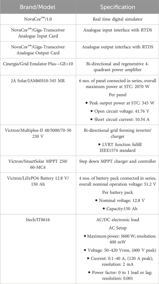
Table 1. PHiL Setup 1—Real time simulator and grid emulator specifications.
In terms of implementation, it is practical to adopt a phased approach. Starting with pilot projects that focus on smaller sections of the grid or specific types of inverters can help refine the methodologies and provide valuable insights into their effectiveness and cost implications. Following successful pilot tests, these technologies can be gradually scaled to larger sections of the grid. Additionally, integrating PHIL and DT with existing grid management systems and data analytics tools can optimize the investment by leveraging existing infrastructures, thus reducing the need for entirely new systems. While the implementation of PHIL and DT in large-scale grid settings with massive numbers of inverters is complex and costly, the strategic benefits in terms of enhanced performance, reliability, and potential cost savings make it a compelling investment. Careful planning and phased implementation are crucial to managing costs and maximizing the efficiency and return on these technological investments.
By conducting PHIL and DT tests on GFM inverters, we gain invaluable insights into their potential, optimizing their design and control strategies to meet the evolving demands of modern power systems. This ensures the transition towards a future with a higher reliance on renewable energy sources, our electrical grids remain robust, adaptive, and resilient, supported by the advanced capabilities of grid-forming inverters.
2 Digital Twin
DT technology is increasingly viewed as a vital tool in meeting the demands of power system decarbonization, offering advanced capabilities for the planning, monitoring, and operation of future energy infrastructures. A DT is essentially a dynamic, virtual model that mirrors a physical system, enabling a real-time representation of system behaviour. The components of a DT-based system include the virtual model itself, the physical system it emulates, the communication pathways between the two, the data exchanged, and the DT services that support various applications.
Distinct from traditional static models, a DT defining characteristic is its integration with live data streams, which allows it to reflect the instantaneous state of the physical system. Depending on the application’s requirements and design specifications, DT models can emphasize different aspects, such as electrical characteristics, physical geometry, thermal dynamics, or mechanical movements. For industry-wide adoption of DT to gain momentum, it is critical to develop and validate them within realistic test environments (Uhlemann et al., 2017). Although the research realm has made considerable strides in real-time simulations and PHIL testing, DT present unique challenges. These include the necessity for a seamless data connection between the physical asset and its virtual counterpart, and the potential for performance issues arising from communication latency and data throughput.
Implementing DT technology in power systems presents several challenges, such as communication delays, data integration complexities, and maintaining real-time synchronization between the physical system and its digital counterpart. Each of these issues requires specific solutions to ensure the efficacy of the DT in real-time operations and decision-making.
Communication delays are a significant challenge, particularly in scenarios where real-time data transmission is critical for system stability and decision-making. Delays can occur due to the physical distance between data sources and processing centers, legacy communication infrastructure, or bandwidth limitations. To address these, network optimization is crucial, which involves upgrading to faster, more reliable data transmission lines such as fibre-optic communications. Additionally, implementing edge computing can minimize delays, as data processing occurs closer to where it is generated. Advanced communication protocols designed for real-time applications, like MQTT or CoAP, also help in reducing latency.
Another challenge is integrating disparate data types and sources, which is essential for the DT’s operation. This complexity can be managed through data standardization, which involves adopting common data formats and communication standards. Middleware solutions can serve as an intermediary layer to facilitate data integration by translating between different data formats. Furthermore, employing advanced analytics and machine learning algorithms can enhance the process of data cleansing, integration, and analysis, ensuring the reliability of the data used for decision-making.
Maintaining real-time synchronization between the DT and the physical system is crucial. Any delay or lag in mirroring the physical system’s state can lead to incorrect decision-making. To overcome this, ensuring that all data used by the DT is time-stamped allows the system to account for any delays and process the most relevant and recent data snapshot. The use of Real-Time Operating Systems (RTOS) is beneficial in managing data in real-time, ensuring that the DT remains synchronized with the physical system. Additionally, establishing continuous feedback loops between the physical system and the DT helps in continuously adjusting and recalibrating the model based on the latest data and insights.
By addressing these challenges with targeted technological solutions and strategic system design, DT technology can be effectively implemented to enhance decision-making and operational efficiency in power system restoration and management. These solutions not only solve the immediate problems but also enhance the overall resilience and adaptability of the power systems to future challenges. In this study, a bespoke testing platform is proposed. This platform is tailored to the specific operational needs of DT, integrating a software-based communication emulator to replicate the data interactions between the physical system and the DT. This approach ensures that the DT performance is evaluated under conditions that closely mimic its intended real-world application, thus providing a robust foundation for the deployment of this transformative technology in the energy sector.
2.1 DT system modelling
A PV system, AC-coupled BESS, MPPT and aggregate load, are connected to the RTDS. The hierarchy box with the corresponding equipment images represents the sub-system internal circuit and control topologies. The microgrid is capable of operating in both islanding mode and grid-connected mode (Malakuti et al., 2019). The PV system design includes a photovoltaic cell/array module, an inverter, a filter, and a circuit breaker. The PV array is designed to have an overall open circuit voltage of 1.432 kV and a short circuit current of 960 A. At Standard Test Conditions (STC), this configuration is capable of producing approximately 1 MW of power.
2.2 Photovolatic system model
The output produced by the PV module is in the form of currents and voltages. The PV module produces an IV curve (current-voltage) and a P-V curve (power and voltage). Every PV module has this characteristic, which can be expressed as follow:
Where Iph is the short circuit current, Is the reverse saturation current of the diode, q is the electron charge (1,602 × 10−19 C), V is the diode voltage, k is the Boltzman constant (1,381 × 10−23 J/K), T is the junction temperature, N is the ideal factor of the diode, Rs is the series ground of the diode, and Rsh is the shunt resistance of the diode.
A photovoltaic cell consists of a p-n junction fabricated in a thin layer of semiconductor. When the incident radiation is low, the output I-V characteristics of a photovoltaic cell have an exponential characteristic similar to that of a diode. However when the radiation is higher, photons with energy greater than the bandgap energy across the p-n junction and a current proportional to the incident radiation is generated. When the cell is connected to an external load at the terminals, these current flows in the external circuit or else is shunted internally by an intrinsic p-n junction diode (Wang et al., 2013). Hence, it can be seen that the diode characteristics sets the open circuit voltage characteristics of a solar cell. A PV cell can thus be modelled as a current source in parallel with a diode with the output of the current source (current generated by the PV cell) proportional to incident Sun radiation, and the temperature dependence, quality factor and resistance of the diode (Letcher, 2022).
The formula used:
where
IL is the current generated due to Sun radiation.
IO is the diode saturation current.
η is the diode quality factor.
RS is the series resistance of the PV cell.
k is the Boltzmann's constant given by 1.38 × 10⁻²³
q is the charge constant and is equal to 1.6 × 10⁻¹⁹
G is the Sun radiation in W/m2.
T1 is the nominal temperature in °C.
Gnom is the nominal Sun’s radiation used for the modeling, obtained from manufacturer’s data.
ISC is the short circuit current through the PV diode.
VOC is the open circuit voltage of the panel, obtained from manufacturer’s data.
Formulas (1–8) are imputed in the DT model for simulation.
To simulate real-time solar irradiation, a slider is provided at runtime to control the intensity of the sunlight. Additionally, a rate limiter is connected after the slider to accurately represent the shading effect (Thijssen et al., 2018). This allows for precise adjustments of the solar irradiation, taking into account factors such as clouds or obstructions that may partially block the sunlight. Below Figure 1 shows the detailed PV control model.
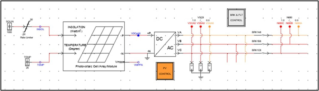
Figure 1. Detailed PV control model.
2.3 Battery energy storage system
The BESS serves as a repository, a grand library of electrons, where the bounty harvested from solar PV arrays is stored. The solar energy, once captured by the PV panels, is converted from its primal form, direct current (DC), into a more versatile form, alternating current (AC), through the mystical arts of the inverter, it can then be stored within the BESS, to be called upon when the Sun’s grace is obscured by night or cloud. The BESS system is considered as 4 batteries connected with series with each 12.8 V/150 Ah for microgrid operation. The energy released by the BESS can be calculated with formula 9-11 (Letcher, 2022).
where
Expdenotes Bess’s exponentially zone voltage(V), and Q = Bess capacity(Ah),
The block model and DT diagram is shown in Figures 2, 3.
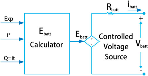
Figure 2. Block model of Bess.
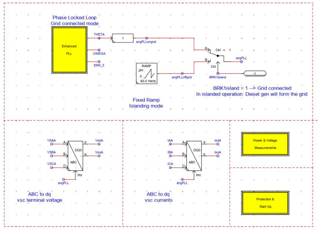
Figure 3. Detailed DT model of BESS.
By incorporating these control components and blocks, the BESS control scheme ensures effective regulation, protection, and monitoring of the energy storage system. It enables optimal operation, efficient power flow, and adherence to safety and stability requirements (Li et al., 2016).
The BESS system can function in both island mode and grid connection mode through the use of a three-phase PLL (Phase-Locked Loop). In this system, a three-phase voltage is supplied to the multiplier, which acts as a phase detector (Mohanty et al., 2016). The phase difference signal obtained from the multiplier is then transmitted to a VCO (Voltage-Controlled Oscillator), similar to a traditional single-phase PLL.
The VCO processes the phase difference signal and generates a three-phase sinusoidal signal, ensuring that it is synchronized with the grid or the reference voltage. Additionally, the VCO introduces a corresponding phase shift to align the BESS output with the grid voltage or the desired operating conditions.
By employing this three-phase PLL, the BESS can effectively regulate its operation and maintain synchronization with the grid in grid connection mode, or maintain stable operation in island mode when disconnected from the grid. The PLL ensures that the BESS output voltage and frequency are consistent with the grid or the desired reference, enabling smooth and reliable operation of the system.
Two control loops–P-Q control and Voltage control are implemented in grid connection and islanded mode and shown in below Figure 4.
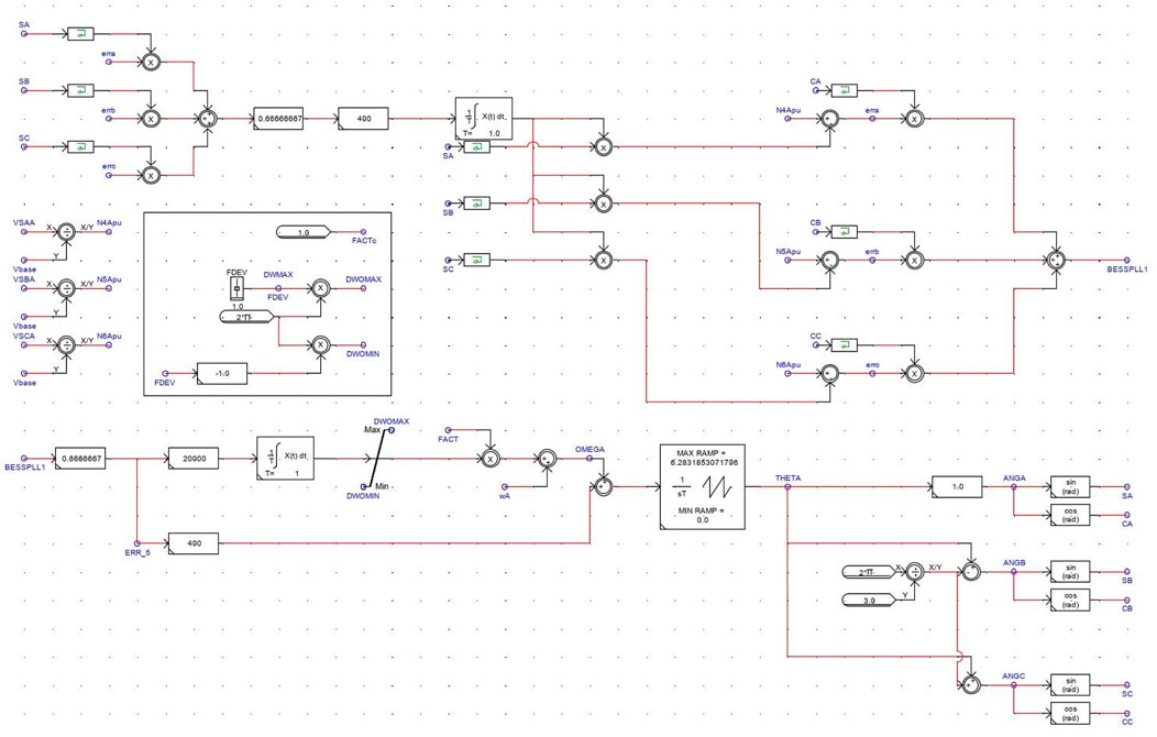
Figure 4. P–Q control and voltage control platform.
2.4 Grid-forming inverter
Grid-forming (GFM) inverters are crucial in power restoration, especially in scenarios where the existing grid infrastructure is unavailable or unstable. These inverters do not merely follow the existing grid parameters; instead, they actively establish and control the grid’s voltage and frequency. This capability is critical during power restoration, as it allows GFM inverters to provide a stable reference for other systems to synchronize with, effectively facilitating the reconnection of the grid.
The primary control strategy employed by GFM inverters is voltage and frequency control via droop control. This strategy involves adjusting the output frequency and voltage of the inverter based on the load it experiences. For instance, an increase in load typically leads to a slight reduction in output frequency and voltage, helping maintain stability across the grid. This behaviour is similar to traditional generators and is vital during the variable load conditions often present during the initial phases of power restoration. Furthermore, GFM inverters contribute virtual inertia and damping to the grid. Virtual inertia provides resistance against changes in frequency, mimicking the inertia inherent in conventional rotating generators. This feature is essential for damping frequency fluctuations following disturbances. Similarly, virtual damping adds resistance to rapid changes in power flow, aiding in voltage stabilization post-fault or during significant load changes. These capabilities are critical for maintaining grid stability and ensuring a smooth restoration process.
Parameter optimization is a crucial aspect of deploying GFM inverters effectively. Key parameters include droop coefficients for frequency and voltage, the inertia constant, and the damping factor. These parameters are not universally fixed and must be tailored to the specific dynamics of the grid and its operational demands. For example, a grid with a high renewable energy mix and frequent load changes might require different settings compared to a more stable grid with traditional power generation.
For the Grid Forming Inverter model, droop control topology is adopted. The inverter can be approximated as an idea voltage source with Eqs 12–14,
providing power to another source (terminal),
via an impedance.
The impedance, represented by the resistive component Rc and the inductive component Lc, functions as a simplified representation of a transformer’s characteristics. This model is instrumental in establishing the connection between the inverter and the electrical grid at their point of intersection (Qoria et al., 2020). Under conditions of system stability, both the grid’s voltage and the inverter’s output maintain sinusoidal waveforms, each oscillating at their respective native frequencies, symbolized by
The P and Q powers being delivered by the source are calculated using load voltage and output current measurements, as expressed by and below as:
where, δ denotes the power angle. It is observed that when
This forms the basis of droop control principle in parallel-operated power systems, whereby, P∼δ and Q∼E. Hence, it gives rise to conventional droop control strategy denoted by as:
where E∗ and ω∗ represent the rated values of voltage and frequency, respectively.
The droop coefficients are designed by as follows:
the selection of the droop coefficients, shown in Eqs 21, 22, represented by m for frequency and n for voltage, is a calculated decision based on the specific needs of the system. These needs include the required responsiveness of frequency and voltage to alterations in power and the imperative for equitable power distribution amongst a cohort of parallel inverters. These coefficients are pivotal in defining the degree to which frequency and voltage will deviate in response to fluctuations in power.
The droop parameters are meticulously calibrated so that an increase in power output by a single inverter results in a modest reduction in both its frequency and voltage. This subtle decline acts as a signal to the remaining inverters, compelling them to modulate their output. This orchestration is crucial for upholding the equilibrium of the load and for ensuring that the grid’s frequency and voltage remain within the bounds of acceptability.
For GFM inverters, droop control is a cornerstone for distributed control mechanisms that underpin power equalization and grid robustness. This technique is exceedingly beneficial within microgrid architectures or in contexts where the integration of renewable energy sources into the power matrix is pursued (Singh et al., 2024). It warrants mention, however, that the practical application of droop control encompasses complexities beyond the basic principle, often necessitating added components and regulatory circuits to refine the dynamic response and to guarantee steadfast stability across a spectrum of operational states.
2.5 MPPT
Maximum Power Point Tracking (MPPT) is a technique used in PV systems to maximize the energy harvest from the solar panels. Solar panels have non-linear voltage-current characteristics, which means that the power output is dependent on the operating voltage and current (Maeng et al., 2024). The Maximum Power Point (MPP) is the point on the voltage-current (V-I) curve of a solar panel at which the product of current (I) and voltage (V) is maximized, resulting in the highest possible power output (P). The goal of MPPT is to adjust the operating point of the solar panels to the MPP, especially since this point changes with varying environmental conditions such as temperature and irradiance. When adopting the MMPPT into the DT model, the following algorithms are implemented within the solar inverter or a dedicated charge controller.
Where VmppM is the maximum voltage at the peak to peak of the PV module circuit, Ns is the series circuit, VmppM is the peak voltage value.
Where Imppm is the maximum current generated by a PV system, Np is a total of parallel circuit, and Impp is the maximum current generated by one to PV module, as shown in Eq. 23. Thus, the series of PV modules can produce the following V-I and PV characteristic curves is shown in below Figure 5:
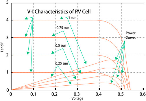
Figure 5. V–I and PV characteristic curves.
In grid-tied configurations, the MPPT’s critical role is within the inverter, while in off-grid setups, it is essential to the charge controller. The operational voltage of a solar panel is affected by the intensity of sunlight exposure, electrical demand, and temperature of the panel itself. Assessing the performance of an MPPT system is crucial for evaluating its efficiency and guiding further improvements. When designing the MPPT block in DT, dynamic parameters and static parameters are taken into account (Jeong et al., 2020). For dynamic parameters, the MPPT’s ability is evaluated to locate the MPP amidst fluctuating environmental conditions, such as changes in cell temperature and solar irradiance. Superior performance is indicated by a quicker response time in identifying the MPP. As for static parameters, the stability of the output power is measured when the MPP has been attained and environmental conditions remain constant. The smaller the deviation in power output, the more effective the MPPT algorithm.
2.6 Real time simulation (RTS)
The use of Electromagnetic Transient (EMT) simulations is becoming increasingly prevalent in the realm of power transmission and distribution. The adoption of real-time simulations, including Hardware-in-the-Loop (HIL) and PHIL, is on the rise for conducting EMT analyses (Edrington et al., 2015). The RTDS, a multiprocessor computing system, is engineered to enhance power system simulation processes. As implied by its name, RTDS is tailored for real-time simulation activities, executing computations that correspond with each passing second of actual time, and it operates in conjunction with physical equipment through the real-time interfacing software.
The core elements of a real-time simulation system encompass parallel processing hardware and specialized input/output cards, such as the Giga-transceiver Analogue Output Card (GTAO) and Giga-transceiver Analogue Input Card (GTAI), which facilitate the connection between external hardware and the simulation environment. The RTDS is recognized for its rapid performance, delivering continuous real-time EMT simulations utilizing the Dommel Algorithm. This algorithm, pioneered by Dr. Hermann Dommel, employs a unique parallel processing structure tailored to address the computational demands of electromagnetic transient simulations. Leveraging this algorithm allows real-time digital simulations to merge the adaptability and precision of digital simulation methods with the instantaneous nature of analogue simulators. The integration of such technology significantly elevates the precision and versatility of the processes used to design, implement, and evaluate control and protection systems for power networks (Sung, 2005). The Eqs 24–26 related to the RTDS calcualtion of equivalent network are shown below:
where
i = current,
v = voltage,
t = given time,
L = inductance,
During each time step, the RTDS Simulator’s parallel processing architecture uses this algorithm to carry out its power system solution process. The user-defined power system is converted to an equivalent network of only current sources and resistors, shown in Figure 6.
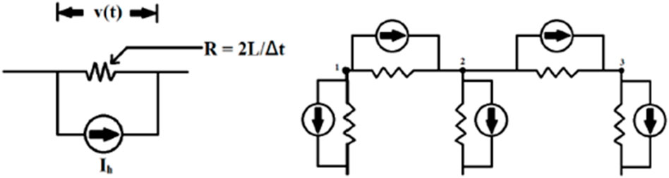
Figure 6. Dommel Algorithm transformation and Dommel Algorithm Equivalent network.
And the conductance matrix is formulated for this equivalent network.
All power system components are represented as equivalent current source and resistor, and then formulate conductance matrix for equivalent network. The conductance matrix is divided into block diagonals that can be treated separately. It should be noted that the simulation time step should be less than traveling time constant
2.7 Grid frequency event emulation
The grid frequency event emulation hierarchy box plays a crucial role in simulating the droop behavior and emulating the primary and secondary frequency control actions of the main grid. Its output signal is transmitted to the controllable voltage source, specifically the AC Type-CC (Constant Current) Control component, in the Microgrid overview frame (Fang et al., 2019). The purpose of this setup is to replicate the behavior of a real grid where the frequency of the system reacts to changes in load or generation. When there is a change in the system, such as an increase in load or a decrease in generation, the grid frequency tends to deviate from its nominal value. The grid frequency event emulation hierarchy box generates a signal that mimics these frequency variations.
The output signal from the grid frequency event emulation hierarchy box is then transmitted to the controllable voltage source, which in turn adjusts its dynamic output frequency based on the received signal (O’Sullivan et al., 2014). This means that the voltage source dynamically responds to changes in the system, such as load or generation fluctuations, by modifying its output frequency accordingly.
By incorporating this mechanism, the simulation model, shown in Figure 7 can accurately represent the frequency response and control actions of a real grid. It allows for a more realistic and comprehensive analysis of the microgrid system, taking into account the dynamic behavior of the voltage source in response to changes in load or generation within the system.
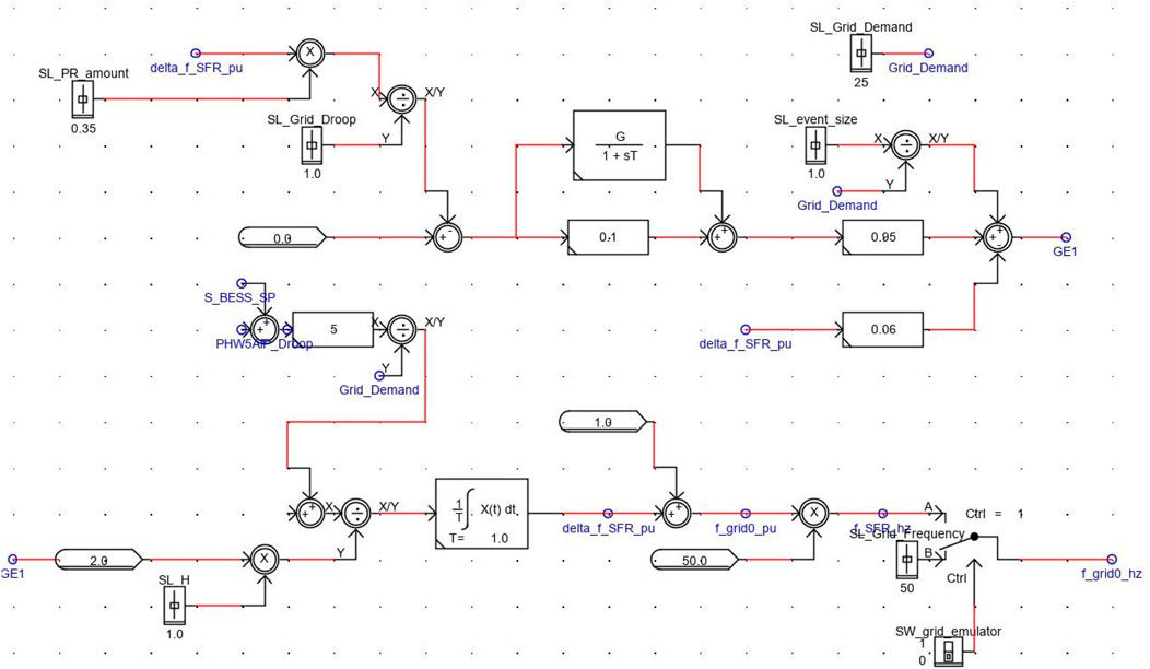
Figure 7. DT simulation model.
2.8 Power Hardware-in-the-loop (setup and parameters)
A comprehensive micro-grid model has been developed, incorporating a variety of components. This model is designed to receive a three-phase power supply and is equipped with mechanisms to control circuit breakers, manage faults, and regulate frequency. The circuit breakers play a crucial role in fault detection and triggering trip signals to address any discrepancies within the grid. In Hong Kong, the micro-grid’s frequency must adhere to the range of 50 Hz ± 2% as specified by the local power utilities’ Supply Rules. Additionally, the micro-grid is designed to generate frequency events, providing valuable insights into the impact of frequency variations.
The micro-grid seamlessly integrates different distributed energy resources, including a PV array, an aggregated load, and an inverter. These components are interconnected to support real-time simulation activities. To ensure continuous monitoring and synchronization between the distributed energy resources and the micro-grid, a Phasor Measurement Unit (PMU) is employed. The ADC/DAC unit plays a critical role in transmitting and receiving control signals to and from the actual hardware, enabling real-time simulation of the grid’s voltage and frequency. Over time, it is possible to monitor changes in the micro-grid’s voltage, frequency, current, active power, and reactive power (Wang et al., 2018).
To mimic frequency variations in the micro-grid, a specialized tool called the grid frequency event emulator is utilized. This tool reflects the balance between the supply of electrical power and the demand, where an increase in demand leads to a drop in micro-grid frequency, and vice versa. Within the PHIL experiment, PV inverters are considered a significant power source that influences the micro-grid’s frequency. Sudden spikes in demand, electrical outages, or disruptions can alter the grid’s frequency, impacting the overall balance. PV inverters play a vital role in maintaining uninterrupted functioning of the micro-grid. Through PHIL testing, issues related to grid system stability can be explored without risking real-world hardware. The primary objective of this research framework is to prevent blackouts and ensure a consistent and reliable power flow to users (Steinmetz et al., 2018).
The model employs a frequency droop control technique, a widely used method for managing the electrical grid’s frequency by adjusting generator outputs in response to load changes. Each generator is assigned a “droop” parameter, which determines the extent to which its output should decrease as the grid frequency increases. When the frequency decreases due to increased load, the generators increase their output to counteract the frequency droop. The contribution of each generator is finely adjusted based on its droop setting, ensuring a fair distribution of increased output across the grid. In PHIL experiments, the grid’s frequency droop signal can be manipulated using a slider linked to the grid event. Additionally, a slide bar allows for precise adjustments of the micro-grid’s frequency through an on/off signal from the frequency emulator.
Regarding the PV array, it is assumed that the irradiance remains constant at 1,000 W/m∧2, and the ambient temperature is fixed at 25°C. A rate limiter is used to restrict the change in irradiance rate, enhancing the accuracy of the simulation by reflecting real-world conditions more effectively. Circuit breakers and fault control points are introduced to simulate faults on the micro-grid’s AC side, aiding in stability assessments under various scenarios. In micro-grid connection mode, a changeover mechanism switches to one terminal, while in islanding mode, it switches to another, ensuring continuous operation of the PV array. However, for safety reasons, renewable energy sources, including PV arrays, are prohibited from operating in islanding mode in Hong Kong. In the event of a circuit breaker trip in islanding mode, a ramp islanding mode signal is employed to maintain the PV array’s operation (Vodyakho et al., 2012).
The outer loop control of micro-grid connection integrates MPPT to optimize the power output of the PV array. This is achieved by identifying the optimal point on the current-voltage curve, considering factors such as temperature, shade, and irradiation effects. Attaining the maximum power point is crucial for the efficient functioning and optimal energy utilization of the PV array within the micro-grid system. The PHIL setup is shown in below Figures 8, 9. The auxiliary devices specification for PHIL setup is shown in Table 2.
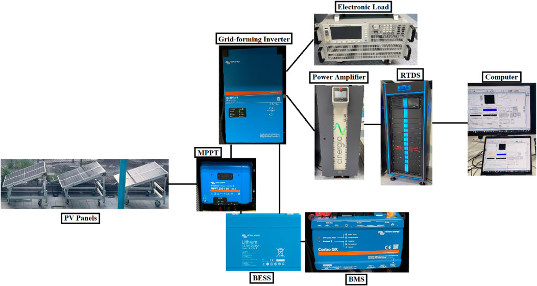
Figure 8. PHIL setup 1
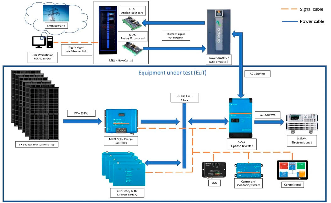
Figure 9. PHIL setup 2

Table 2. PHIL Setup - Auxiliary devices specification.
2.9 Comparison between PHIL and DT
Table 3 below provides a structured comparison to help understand where each technology excels and how they can be complementary. For instance, while PHIL provides precise validation for individual hardware components within a real-time setting, DT allows for broader system-level simulations and optimizations that can inform larger scale operational decisions.
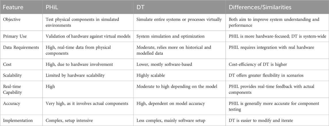
Table 3. Differences and similarities between PHIL and DT.
Traditional grid simulation methods like MATLAB & Simulink, based on software models, often do not fully capture the dynamic interactions of physical components in real-world scenarios. In contrast, the PHIL approach integrates actual hardware into simulations, providing a more dynamic and realistic testing environment. This allows for real-time data acquisition and response, improving the accuracy and realism of tests.
3 Case studies
3.1 Case 1—GFM inverter under three-phase symmetrical fault (2-s)
In Case 1, both the DT Model and PHIL system are run with the aid of real-time digital simulator to test out the performance of GFM inverter under three-phase symmetrical fault. Figure 10 and Figure 11 show the voltage and frequency change in grid-forming inverter when encounter three-phase symmetrical fault (2-s):
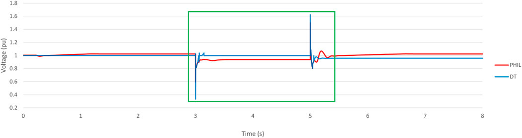
Figure 10. Voltage change in grid-forming inverter when encounter three-phase symmetrical fault (2-s).
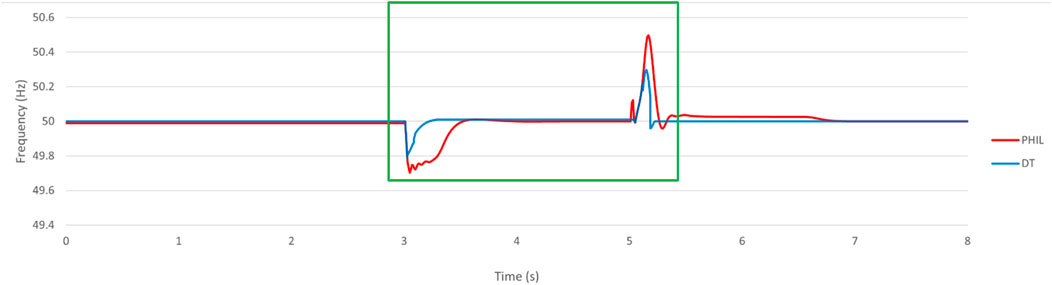
Figure 11. Frequency change in grid-forming inverter when encounter three-phase symmetrical fault (2-s).
The voltage of the system was stabilized at 1 per unit (pu) prior to the occurrence of an event. At 3 s, a symmetrical fault happened, resulting in a voltage dip in both the PHIL and DT simulated systems. Following the event, the load voltage dropped to 0.59pu and 0.38pu, and then recovered to 0.9pu in 580 ms and 402 ms, respectively. After 2 s, the fault was cleared, causing a disturbance in the system. The load voltage increased to 1.49pu and 1.62pu. Following that, the system’s disturbance rejection mechanism rapidly attenuated the voltage to 1.1pu in 26 ms and 19 ms respectively. Afterward, the system achieved the quasi-steady state, and eventually stabilized after the event.
Prior to the occurrence of an event, the load frequency was stabilized at 50 Hz. At the 3-s mark, a symmetrical fault occurred, causing a drop in frequency in both the PHIL and DT simulated systems. As a result of this event, the load frequency decreased to 49.70 Hz and 49.78 Hz. The frequency then recovered to its nominal value within 490 ms and 190 ms in the PHIL and DT systems, respectively. After a duration of 2 s, the fault was cleared, leading to an increase in the load frequency to 50.49 Hz and 50.3 Hz in the PHIL and DT systems, respectively. Subsequently, the load frequency control loop quickly mitigated the frequency disturbance, allowing the system to achieve steady state within 530 ms and 138 ms in the PHIL and DT systems, respectively.
3.2 Case 2—GFM inverter encountered Loss of Main
In Case 2, both the DT Model and PHIL system are run with the aid of real-time digital simulator to test out the performance of GFM inverter under LoM. Figure 12 and Figure 13 show the voltage and frequency change in grid-forming inverter when encounter LoM:
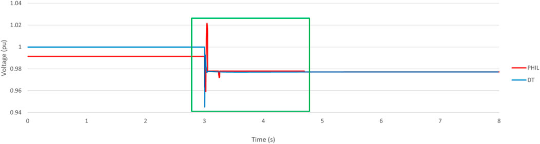
Figure 12. Voltage change in grid-forming inverter when encounter LoM.
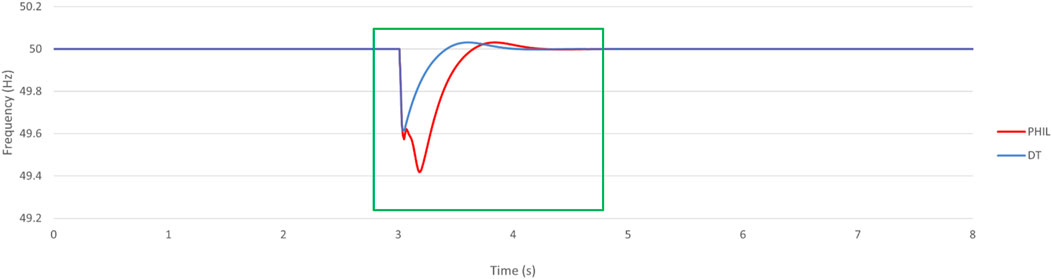
Figure 13. Frequency change in grid-forming inverter when encounter LoM.
Before the Loss of Main event occurred in the PHIL and DT systems, the load voltage of the was stabilized at 0.991 pu and 1 pu. When the system was islanded at 3 s, the load voltage exhibited fluctuations. In the PHIL system, the voltage bounced between 1.022 pu and 0.959 pu, while in the DT system, it varied between 1 pu and 0.945 pu. Fortunately, both systems quickly recovered to their nominal voltage levels within a short time period. The PHIL system took 52 ms to stabilize, whereas the DT system took 15 ms.
Prior to the onset of Loss of Main event, the system’s frequency was maintained at a stable 50 Hz. However, when the LoM occurred at the 3-s mark, the system experienced a reduction in inertia, resulting in a significant deviation from the target frequency. Consequently, the load frequency dropped to 49.42 Hz in the PHIL system and 49.62 Hz in the DT system. In response to this frequency deviation, the load frequency control loop promptly initiated corrective measures by increasing the active power generation. This action aimed to restore the system’s frequency to its nominal value. The control loop exhibited efficient performance, successfully attenuating the frequency disturbance and achieving frequency restoration within a relatively short timeframe. Specifically, the PHIL system recovered to the target frequency in 653 milliseconds (ms), while the DT system accomplished the same in 477 ms.
3.3 Case 3—GFM inverter encountered Loss of Main (improved case study—Apply Perez model)
By comparing the result from the DT model and PHIL system in the above case studies, they show similar behaviour on frequency and voltage. The data in PHIL system shows more realistic result in the case studies 1 & 2. By exchanging data between the PHIL system and the DT model, improvement can be made to enhance the DT system.
Solar irradiance stands as the primary factor influencing the temperature projections for PV modules and the exactitude of such irradiance values is vital for the refinement of the DT model.
By utilizing Perez model in the DT model, the diffuse irradiance on a tilted plane from the known values of global horizontal irradiance, the geometry of the Sun and the plane can be estimated. The model separates the sky into two primary components, including isotropic diffuse radiation which represent the uniform sky component that is unaffected by the Sun’s position and anisotropic diffuse radiation which represent the sky’s non-uniform component depending on the Sun′s position.
The total diffuse irradiance (Id) on a tilted plane can this be expressed as the sum of these two components, shown in Eq. 27 below:
where:
Idiso is the isotropic diffuse irradiance component.
Idaniso is the anisotropic diffuse irradiance component including circumsolar and horizon-brightening components.
The isotropic component Idiso is calculated with Eq. 28 below:
where: Idh dh is the diffuse horizontal irradiance.
The anisotropic component Idaniso is further broken down into the circumsolar and horizon brightening components, using Eq. 29 below:
where:
F1, F2 and F3 are coefficients that account for the circumsolar and horizon brightening effects, which are functions of the solar zenith angle, the sky clearness, and the sky brightness. 0 is the solar zenith angle.
The coefficients F1, F2 and F3 are determined from empirical data and are often presented in tabulated form within the literature for different values of sky clearness and brightness. The clearness index Kt and the brightness index Zb are used as inputs to obtain these coefficients from the tables or empirical equations.
Finally, the model also accounts for the reflected component from the ground with Eq. 30 below:
where:
Igh is the global horizontal irradiance.
Thus, the total irradiance on the tilted surface is the sum of the direct, diffuse, and reflected components, shown in Eq. 31 below:
Where
By applying the Perez model with its empirical coefficients and detailed consideration of the various components of solar irradiance, the DT model can be more precise, the following figures Figure 14 and Figure 15 show the performance of integrated model under LoM:
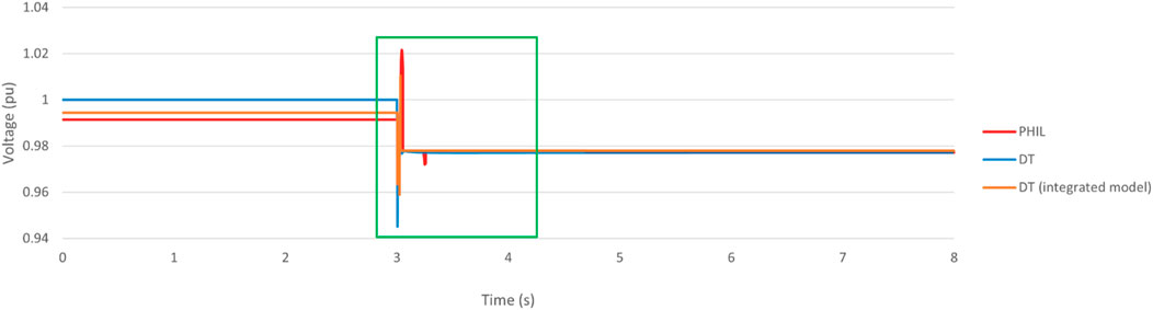
Figure 14. Voltage change in integrated model when encounter LoM.
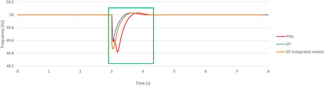
Figure 15. Frequency change in integrated model when encounter LoM.
As a result, the integrated DT model’s load frequency at the minimum point is 49.47 Hz, which is much closer to the PHIL model. Additionally, the frequency recovery time is 532 ms, indicating that the acceleration parabola time constant is relatively similar to the PHIL environment. Moreover, the steady-state load voltage of the integrated DT model is 0.994pu, which is also closer to the PHIL environment. However, it is worth noting that the voltage bounds between 1.011pu and 0.960pu, showing a closer resemblance to the behaviour of the PHIL system.
4 Discussion
This paper presents a real-time simulation on both physical and digital platforms of grid-forming inverter under LoM and three-phase fault. From the result of case 1 and 2, the GFM inverter shows similar behaviour in both PHIL system and DT model.
For case 1, before any disruptions, the system’s voltage was precisely maintained at the nominal level. Upon the occurrence of a symmetrical fault at a specific moment during the simulation, both the PHIL and DT systems experienced a notable voltage drop. This was followed by a prompt voltage recovery to near-nominal values in a fraction of a second for both systems. Once the fault was cleared after a brief interval, an overvoltage condition was observed, after which the systems’ rapid disturbance rejection responses quickly brought the voltage back to a slightly elevated level compared to the nominal setting. The systems then transitioned to a quasi-steady state and ultimately regained voltage stability after the disturbance. Simultaneously, the load frequency had been stable before the event. The same fault led to a slight decrease in frequency in both the PHIL and DT simulations. The frequency then returned to its standard value swiftly. Post-clearance of the fault, a brief frequency overshoot occurred, which was promptly corrected by the load frequency control mechanisms. The systems achieved a steady operational frequency shortly thereafter.
For case 2, prior to the LoM event, the PHIL and the DT simulations were operating with a high degree of voltage stability. The load voltage was finely tuned to just below and at unity in the respective systems. However, the stability was challenged at the moment the systems transitioned into an islanded state. This changeover, occurring at a decisive moment, initiated a series of voltage fluctuations. Within the PHIL system, the voltage oscillated slightly above and below the nominal level, while the DT system experienced a similar, albeit slightly wider, range of voltage variation. Despite these perturbations, both systems demonstrated remarkable resilience and agility in restoring voltage equilibrium in an expedient manner, with the PHIL system requiring slightly over half a second and the DT system even less to achieve stability. Simultaneously, the system’s frequency, which had been consistently held at 50 Hz, was impacted by the LoM event. The sudden reduction in system inertia precipitated a tangible deviation from the set frequency value. This led to a modest drop in the operating frequency of both systems. To counteract this deviation, the load frequency control loop sprang into action, enhancing active power output as a corrective measure to reel the frequency back to its designated threshold. The efficiency of the control loop was evident in its swift response, successfully dampening the frequency disturbance and returning to the target frequency within a short span—markedly under a second for both systems. This rapid restoration underscores the systems’ robust frequency regulation capabilities, which are essential for maintaining grid stability under dynamic conditions and ensuring reliable operation amidst potential disruptions.
For case 3, by incorporating the Perez model within the DT framework enhances the system’s ability to precisely estimate diffuse irradiance on a tilted surface. This estimation is informed by recognized measurements of global horizontal irradiance, in conjunction with the precise geometric relationship between the Sun and the plane in question. The Perez model is particularly adept at dissecting the sky’s radiation into two fundamental elements: isotropic and anisotropic diffuse radiation. The isotropic component is characterized by a uniform distribution that remains constant, irrespective of the solar position. It captures the portion of the sky’s diffused light that is evenly scattered across the heavens. On the other hand, the anisotropic component of diffuse radiation is sensitive to the location of the Sun, capturing the complexity of the sky’s luminance that varies with the Sun′s trajectory.
By leveraging the Perez model, the DT system gains an intricate understanding of how sunlight interacts with surfaces at various orientations and angles throughout the day. This nuanced simulation of solar irradiance is crucial, as it feeds into the overall accuracy of the system’s energy predictions and performance assessments. It enables a more realistic replication of the physical environment within the DT, providing valuable insights into the impact of solar radiation on energy production and system behavior. This, in turn, solidifies the DT model’s role as an indispensable tool for forecasting and optimizing the operation of solar-dependent energy systems, ensuring that they can efficiently adapt to the ever-changing patterns of sunlight exposure. The final simulated shows that the data exchange between physical and digital systems can spot out the elements which can be integrated, which can eventually increase the accuracy of the digital system.
5 Conclusion
In conclusion, the swift paradigm shift towards a decarbonized power grid, underpinned by the proliferation of DERs, presents a dual-edged sword. While it aligns with global sustainability goals, it simultaneously imposes significant challenges on grid stability due to the limited transparency in DER operations. The implications of these challenges resonate through the risk of overwhelming the grid’s capacity, thereby necessitating innovative solutions to preserve the integrity of the energy network.
DT technology emerges as a critical solution to these challenges. By crafting virtual replicas of the physical grid infrastructure that require minimal data transmission, DTs significantly diminish the barriers imposed by the demands of real-time data flows. This advancement not only enhances the visibility of the grid’s operational dynamics but also provides a strategic platform for grid optimization and resilience. The paper underscores the urgency of adopting DT technology within the energy sector and stresses the importance of validating its effectiveness through empirical demonstrations. It showcases a dedicated simulation platform that seamlessly integrates DT and PHIL methodologies. This hybridized platform serves as a testbed for prototyping and validating grid-forming inverters—a cornerstone in the quest for robust power restoration solutions.
This research marks a significant advancement in the integration of PHIL & DT technologies for the power systems sector. It innovatively combines real-time hardware simulation with dynamic system modelling to form a strong framework for testing, analysis, and system restoration. Moving beyond traditional DT technologies that focus on virtual simulations, this study incorporates real hardware into the loop, enhancing the accuracy and practicality of how components interact under simulated conditions. The integration is particularly transformative in system restoration, a complex area crucial for managing large-scale disruptions in power grids. The PHIL-based DT setup allows for risk-free simulation and testing of restoration strategies, mimicking real-world conditions. This capability provides grid operators and engineers with a powerful tool to plan, test, and optimize restoration procedures effectively and confidently. The ability to simulate various failure scenarios and restoration strategies using real hardware within a DT framework deepens the understanding of system vulnerabilities and recovery options, significantly enhancing the resilience and efficiency of power systems.
Furthermore, the integration of the Perez Model within the DT framework represents a leap forward in enhancing the fidelity of simulations. By capturing the nuanced interplay between solar irradiance and grid performance, the model fine-tunes the DT’s predictive capabilities, ensuring a closer alignment with the physical realities captured by PHIL experiments.
The necessity for future research into DT and PHIL technologies is highlighted by the evolving complexity of modern power systems. Key areas for further investigation include scalability, where research should focus on managing data from diverse sources for larger-scale simulations. Another critical area is the integration of renewable energy sources, requiring improvements in predictive models to manage their variability. Cybersecurity is also paramount, with a need for advanced protocols to protect data and ensure the reliability of DT. Additionally, advancements in real-time data processing using artificial intelligence could enhance decision-making capabilities. Economic and regulatory research is crucial to understand the cost implications and necessary policy adjustments for broader adoption.
In PHIL, refining validation techniques is essential to ensure simulations accurately reflect real-world conditions. Research into interoperability and the development of advanced visualization tools, like augmented or virtual reality, could improve how these technologies are integrated and utilized. Each of these areas offers significant potential to advance the capabilities and applications of DT and PHIL technologies in modern power systems.
In the broader context, this paper’s findings illuminate a path toward a more transparent, adaptable, and sustainable power grid. The successful application of DT and PHIL technologies in tandem has the potential to revolutionize grid management practices. It paves the way for a future where grid operators can anticipate and respond to the intricacies of a renewable-heavy energy landscape with unprecedented precision and confidence. Hence, the research presented here not only contributes to the academic discourse but also provides actionable insights for industry stakeholders striving to navigate the complexities of an evolving energy paradigm.
Data availability statement
The raw data supporting the conclusions of this article will be made available by the authors, without undue reservation.
Author contributions
MC: Conceptualization, Data curation, Formal Analysis, Funding acquisition, Investigation, Methodology, Project administration, Resources, Software, Supervision, Validation, Visualization, Writing–original draft, Writing–review and editing. KL: Data curation, Investigation, Methodology, Resources, Software, Validation, Writing–review and editing.
Funding
The author(s) declare that no financial support was received for the research, authorship, and/or publication of this article.
Conflict of interest
The authors declare that the research was conducted in the absence of any commercial or financial relationships that could be construed as a potential conflict of interest.
Publisher’s note
All claims expressed in this article are solely those of the authors and do not necessarily represent those of their affiliated organizations, or those of the publisher, the editors and the reviewers. Any product that may be evaluated in this article, or claim that may be made by its manufacturer, is not guaranteed or endorsed by the publisher.
References
Chen, J., Si, W., Liu, M., and Milano, F. (2023). On the impact of the grid on the synchronization stability of grid-following converters. IEEE Trans. Power Syst. 38 (5), 4970–4973. doi:10.1109/TPWRS.2023.3284262
Dong, D., Wen, B., Boroyevich, D., Mattavelli, P., and Xue, Y. (2015). Analysis of phase-locked loop low-frequency stability in three-phase grid-connected power converters considering impedance interactions. IEEE Trans. Ind. Electron. 62 (1), 310–321. doi:10.1109/tie.2014.2334665
Edrington, C. S., Steurer, M., Langston, J., El-Mezyani, T., and Schoder, K. (2015). Role of power hardware in the loop in modeling and simulation for experimentation in power and energy systems. Proc. IEEE 103 (12), 2401–2409. doi:10.1109/jproc.2015.2460676
Fang, J., Zhang, R., Li, H., and Tang, Y. (2019). Frequency derivative-based inertia enhancement by grid-connected power converters with a frequency-locked-loop. IEEE Trans. Smart Grid 10 (5), 4918–4927. doi:10.1109/tsg.2018.2871085
Goksu, O., Teodorescu, R., Bak, C. L., Iov, F., and Kjær, P. C. (2014). Instability of wind turbine converters during current injection to low voltage grid faults and PLL frequency based stability solution. IEEE Trans. Power Syst. 29 (4), 1683–1691. doi:10.1109/tpwrs.2013.2295261
Jeong, J., Shim, M., Maeng, J., Park, I., and Kim, C. (2020). A high-efficiency charger with adaptive input ripple MPPT for low-power thermoelectric energy harvesting achieving 21% efficiency improvement. IEEE Trans. Power Electron. 35 (1), 347–358. doi:10.1109/tpel.2019.2912030
Lawder, M. T., Suthar, B., Northrop, P. W. C., De, S., Hoff, C. M., Leitermann, O., et al. (2014). Battery energy storage system (BESS) and battery management system (BMS) for grid-scale applications. Proc. IEEE 102 (6), 1014–1030. doi:10.1109/JPROC.2014.2317451
Li, X., Yao, L., and Hui, D. (2016). Optimal control and management of a large-scale battery energy storage system to mitigate fluctuation and intermittence of renewable generations. J. Mod. Power Syst. Clean Energy 4 (4), 593–603. doi:10.1007/s40565-016-0247-y
Maeng, J., Jeong, J., Park, I., Shim, M., and Kim, C. (2024). A time-based direct MPPT technique for low-power photovoltaic energy harvesting. IEEE Trans. Industrial Electron. 71 (5), 5375–5380. doi:10.1109/TIE.2023.3288183
Malakuti, S., Schmitt, J., Platenius-Mohr, M., Grüner, S., Gitzel, R., and Bihani, P. (2019). A four-layer architecture pattern for constructing and managing digital twins. Proc. 13th Eur. Conf. Softw. Archit. 11681, 231–246. doi:10.1007/978-3-030-29983-5_16
Meng, X., Liu, J., and Liu, Z. (2019). A generalized droop control for grid-supporting inverter based on comparison between traditional droop control and virtual synchronous generator control. IEEE Trans. Power Electron. 34 (6), 5416–5438. doi:10.1109/tpel.2018.2868722
Mohanty, S., Subudhi, B., and Ray, P. K. (2016). A new MPPT design using grey wolf optimization technique for photovoltaic system under partial shading conditions. IEEE Trans. Sustain. Energy 7 (1), 181–188. doi:10.1109/tste.2015.2482120
O’Sullivan, J., Rogers, A., Flynn, D., Smith, P., Mullane, A., and O’Malley, M. (2014). Studying the maximum instantaneous non-synchronous generation in an island system—frequency stability challenges in Ireland. IEEE Trans. Power Syst. 29 (6), 2943–2951. doi:10.1109/tpwrs.2014.2316974
Qoria, T., Rokrok, E., Bruyere, A., François, B., and Guillaud, X. (2020). A PLL-Free grid-forming control with decoupled functionalities for high-power transmission system applications. IEEE Access 8, 197363–197378. doi:10.1109/access.2020.3034149
Singh, A., Debusschere, V., Hadjsaid, N., Legrand, X., and Bouzigon, B. (2024). “Slow-interaction converter-driven stability in the distribution grid: small-signal stability analysis with grid-following and grid-forming inverters,” in IEEE transactions on power system. (Piscataway: IEEE).
Steinmetz, C., Rettberg, A., Ribeiro, F., Schroeder, G., and Pereira, C. (2018). Internet of Things ontology for digital twin in cyber physical systems. Proc. 8th Braz. Symp. Comput. Syst. Eng., 154–159.
Sun, H., Li, C., Fang, X., and Gu, H. (2017) “Optimized throughput improvement of assembly flow line with digital twin online analytics,” in 2017 IEEE international conference on robotics and biomimetics (ROBIO), Macau, Macao. Piscataway: IEEE, 1833–1837. doi:10.1109/ROBIO.20
Sung, C. O. (2005). Evaluation of motor characteristics for hybrid electric vehicles using the hardware-in-the-loop concept. IEEE Trans. Veh. Technol. 54 (3), 817–824. doi:10.1109/tvt.2005.847228
Thijssen, B. J., Klumperink, E. A. M., Quinlan, P., and Nauta, B. (2018). Feedforward phase noise cancellation exploiting a sub-sampling phase detector. IEEE Trans. Circuits Syst. II Express Briefs 65 (11), 1574–1578. doi:10.1109/tcsii.2017.2764096
Uhlemann, T. H. J., Lehmann, C., and Steinhilper, R. (2017). The digital twin: realizing the cyber-physical production system for industry 4.0. Proc. 24th CIRP Conf. Life Cycle Eng. 61, 335–340. doi:10.1016/j.procir.2016.11.152
Vodyakho, O., Steurer, M., Edrington, C. S., and Fleming, F. (2012). An induction machine emulator for high-power applications utilizing advanced simulation tools with graphical user interfaces. IEEE Trans. Energy Conv. 27 (1), 160–172. doi:10.1109/tec.2011.2179302
Wang, X., Harnefors, L., and Blaabjerg, F. (2018). Unified impedance model of grid-connected voltage-source converters. IEEE Trans. Power Electron. 33 (2), 1775–1787. doi:10.1109/tpel.2017.2684906
Keywords: real time digital simulator (RTDS), digital Twins (DT), Grid-forming inverter, Perez model, power hardware in the loop (PHIL), power restoration, solar photovolatic energy, Smart Grid
Citation: Chow Jason MH and Li Ben KY (2024) Examining grid-forming inverters for power restoration using power-hardware in-the-loop and Digital Twins approaches with Real-time Digital Simulation. Front. Energy Res. 12:1421969. doi: 10.3389/fenrg.2024.1421969
Received: 23 April 2024; Accepted: 08 July 2024;
Published: 30 July 2024.
Edited by:
Shuqing Zhang, Tsinghua University, ChinaReviewed by:
Jiazuo Hou, National University of Singapore, SingaporeHaoming Liu, Hohai University, China
Liang Liang, Harbin Institute of Technology, Shenzhen, China
Copyright © 2024 Chow Jason and Li Ben. This is an open-access article distributed under the terms of the Creative Commons Attribution License (CC BY). The use, distribution or reproduction in other forums is permitted, provided the original author(s) and the copyright owner(s) are credited and that the original publication in this journal is cited, in accordance with accepted academic practice. No use, distribution or reproduction is permitted which does not comply with these terms.
*Correspondence: Man Hin Chow Jason, amFzb25jaG93MjI2QGdtYWlsLmNvbQ==