Refined identification of the key parameters of power system synthesis load model based on the improved butterfly algorithm

With the improvement in power grid simulation accuracy requirements, the existing typical load model parameters can no longer meet the accuracy requirements and become the short board that restricts the stable operation of power system. This paper mainly proposes an improved butterfly optimization algorithm based on the population optimization and dynamic strategy (PODSBOA) for commonly used synthesis load model (SLM) parameters to realize the refined and personalized identification of SLM key parameters:[$p_u$, $q_u$, $R_s$, $X_s$, $R_r$, $X_r$, $K_m$, and $M_{if}$]. The results indicate that in the 2-s load data experiment, the identification error is 0.02, the identification accuracy is 4.09, and the convergence time of the PODSBOA is 12.048 s. In the 5-s load data experiment, the identification error is 0.013, the identification accuracy is 6.65, and the convergence time of the PODSBOA is 23.405 s. The identification errors in the two sets of experiments are reduced by 0.02023–0.06443 compared with other algorithms. The comparison results of different load model parameter identification algorithms indicate that the improved PODSBOA proposed in this paper has high recognition accuracy and fast convergence speed and solves the problem of low accuracy and instability of the identification results of the existing identification schemes.

1 Introduction

The planning, designing, scheduling, and operation decisions of the power system are based on the theoretical support of power system simulation calculation, which is based on the load model of the power system. The accuracy of calculation is closely related to the accuracy of load model parameters. Due to the complex and scattered characteristics of the load, the mathematical model used for the load part in the simulation calculation and analysis of large-scale power systems at this stage is usually based on versatility rather than accuracy. The simulation results obtained by using these rough load models cannot meet the accuracy requirements and the requirements for guiding power system dispatching, operation, and decision-making in the current complex grid environment. In order to ensure the stable operation of the power system, we propose higher requirements for the accuracy of the simulation analysis and calculation of the power system. The load model cannot continue to use typical parameters but needs to establish a new load model for the load nodes through the identification of actual measured data with the short-term and long-term changes in the load (El-Shimy et al., 2018; Kosterev et al., 1999).

At this stage, modeling by identification is gradually becoming the mainstream modeling method, but there are still some problems in obtaining accurate load model parameters through identification (Ma et al., 2008). Power system simulation analysis and decision-making pay more attention to the overall characteristics of load clusters. However, due to the complexity of load characteristics in the actual power grid and the huge differences between different nodes, it is difficult for the load model to accurately describe the overall load characteristics and have good generalization ability in different operating environments in practical applications. It is mainly reflected in two aspects: load data and identification parameters. Specifically, there are few measured data and many parameters to be identified in the synthesis load model (SLM), which is prone to the dispersion problem of unstable identification results and limits the accuracy of model parameter identification. Identifying the load model parameters under less known conditions will cause the problem of the model parameters being unable to be uniquely identified or unidentifiable, and when there are too many identified parameters, the model parameter identification results will have dispersion problems (Zad et al., 2017).

In recent years, the research focus in the field of load modeling has gradually developed with regard to the use of multi-source data and the establishment of generalized synthesis load models for wide-area load modeling problems (Zhao et al., 2020; Ju et al., 2007). At this stage, better results have been achieved in terms of positive deterministic model structure and accurate quantitative model parameters through new techniques and multiple methods (Zhou et al., 2018). Based on the SLM structure, the strategy of identifying only part of the parameters has become one of the most important research directions; setting the parameters with low sensitivity or unimportant parameters as typical parameter values can effectively improve the identification speed (Wang and Han, 2010; Yuan et al., 2021). An effective reconfiguration framework can minimize the distribution loss while the energy demand and load change (Mahdavi et al., 2021). An isolated microgrid dynamic economic load-dispatching method based on particle swarm optimization (PSO) algorithms is studied (Jordehi et al., 2020). Bu et al. (2020) proposed a method combining deep learning to adjust parameter weights to efficiently identify parameters. Simulation evolution methods can be used to solve the problem of load model-parameter identification. Intelligent optimization algorithms in simulation evolution methods are increasingly used in model-parameter identification. The introduction of intelligent optimization algorithms such as particle swarm algorithm, genetic algorithm, and butterfly algorithm into the field of power system-load model-parameter identification results in a notable performance (Bai and Jing 2015; Chen et al., 2022; Kang et al., 2021). However, the intelligent optimization algorithm has problems such as insufficient optimization efficiency and easily falls into local optimality. Therefore, how to improve the algorithm is the key to improving the parameter-identification effect of the synthesis load model. In this novel research, swarm intelligence algorithms such as the improved firefly algorithm (Zivkovic et al., 2022; Bacanin et al., 2021) have successfully combined machine learning and been applied to scenarios such as hyperparameter optimization and feature selection. They yield excellent results and show significant potential. They yield excellent results and show significant potential.

In a word, the difficulty of obtaining load identification data and the inherent structure and parameter limitations of the load model make parameter identification very complicated. The problems of the parameters being unable to be uniquely identified or even unidentifiable and the dispersion of identification results need to be solved urgently (Cheng and Ju 2003). In order to obtain more accurate model parameters and improve the practicability of the load model in the actual power grid, based on the overall measurement method and the related technology of identification modeling using the intelligent optimization algorithm, it is necessary to further carry out more specific research on the identification strategy and the model-parameter identification algorithm of the load model to improve the accuracy and stability of the model-parameter identification results and obtain a more accurate load model to improve the accuracy of the power system simulation calculation. In summary, for solving the problems of low accuracy and instability in parameter identification, it is necessary to carry out further research on the identification strategy of load models and model parameter identification algorithms.

Existing parameter identification schemes have problems such as insufficient identification accuracy and instability caused by scattered identification results. This paper solves the above problems. The main contributions are as follows:

(1) The butterfly optimization algorithm (BOA) is improved based on the population optimization strategy and adaptive dynamic parameter strategy. The search performance of the algorithm is optimized; it has higher convergence accuracy and speed than other algorithms.

(2) An identification scheme for key parameters of the SLM is proposed based on the importance of parameters, which improves the stability and accuracy of the identification scheme.

The paper is organized as follows: Section 1 introduces and reviews the research results related to the load model parameter identification of the power system; Section 2 introduces the structure of the traditional SLM and its parameter identification method; then introduces the theoretical principle, optimization strategy, and calculation process of the improved butterfly algorithm; and finally presents the overall process of SLM parameter identification using the proposed improved butterfly algorithm; Section 3 verifies the recognition accuracy, recognition error, and convergence time of the SLM parameter recognition based on practical cases, which confirms the superiority of the method. The proposed identification scheme sets the parameters that are insensitive to the output as typical parameters, which reduces the parameters to be identified, improves the identification accuracy of the model, and solves the problem of result dispersion that is prone to occur in the process of identifying all parameters. The improved butterfly algorithm has a superior effect on the parameter identification of the SLM. It solves the problems of complexity and low accuracy of parameter identification caused by the acquisition of current load identification data and the limitation of the load model structure and parameters.

2 Materials and methods

2.1 Synthesis load model identification

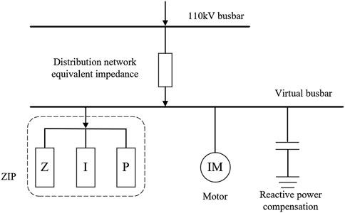
In the actual grid structure, the load is indirectly connected to the substation outlet busbar through the distribution network formed by 110-kV and 35-kV transformers and transmission lines. The load model needs to consider the influence of the impedance in the distribution network at all levels. In order to make the model load characteristics closer to the requirements of the actual grid and to the premise of “qualitative accuracy” of the model structure, the SLM, which directly considers the influence of distribution network impedance, is proposed (Ju et al., 2010; Tang et al., 2009). In the SLM, the actual injected power at the 110-kV node flows into the lower load through the distribution network equivalent impedance, which truly reflects the influence of the impedance in the distribution network.

The SLM consists of six parts in total, as shown in Figure 1, namely, the 110-kV busbar connected to the load model, the distribution network equivalent impedance, the virtual busbar connected to all loads, the static load section (ZIP), the dynamic load section (motor), and the reactive power compensation device (reactive power compensation in the form of capacitors in the model). The equivalent circuit of the synthesis load section in the SLM is shown in Figure 2, where the equivalent circuit port voltage is equal to the virtual busbar voltage $U_L$.

Figure 1

Figure 1. Structure diagram of the SLM.

Figure 2

Figure 2. Equivalent circuit diagram of the synthesis load model.

The third-order induction motor state equation describing the dynamic load of the SLM is shown in Equation 1:

$\left\{\begin{array}{l}\frac{d{e}_{imx}^{\prime }}{dt}=-\frac{1}{T_{d0}^{\prime }}\left[e_{imx}^{\prime }+\left(X-X^{\prime }\right)i_{imy}\right]+s{e}_{imy}^{\prime }\\ \frac{d{e}_{imy}^{\prime }}{dt}=-\frac{1}{T_{d0}^{\prime }}\left[e_{imy}^{\prime }-\left(X-X^{\prime }\right)i_{imx}\right]-s{e}_{imx}^{\prime }\\ \frac{ds}{dt}=\frac{1}{2H}\left(T_M-T_E\right)\end{array}\right..(1)$

The relevant parameters are defined in Equation 2:

$\left\{\begin{array}{l}X=X_s+X_m\\ X^{\prime }=X_s+\frac{X_m{X}_s}{X_m+X_s}\\ T_{d0}^{\prime }=\frac{X_m+X_r}{R_r}\\ \begin{array}{l}{X}_{rm}=X_m+X_r\\ X_p=X_s{X}_r+X_s{X}_m+X_r{X}_m\end{array}\end{array}\right..(2)$

Among them, the electromagnetic torque coefficient and mechanical torque parameters are shown in Equations 3, 4:

$T_E=e_{imx}^{\prime }{i}_{imx}+e_{imy}^{\prime }{i}_{imy},(3)$

$T_M=\left(A{\left(1-s\right)}^2+B\left(1-s\right)+C\right)T_L.(4)$

Among them, $e_{imx}^{\prime }$ is the direct axis component of the transient potential of the induction motor, $e_{imy}^{\prime }$ is the cross-axis component of the transient potential of the induction motor, $i_{imx}$ is the direct axis component of the induction motor current, $i_{imy}$ is the cross-axis component of the induction motor current, $T_{d0}^{\prime }$ is the rotor branch time constant, $H$ is the motor inertia time constant, $T_E$ is the electromagnetic torque, $T_M$ is the mechanical torque, $f$ is the system frequency, $T_L$ is the initial mechanical torque, and $A$, $B$, and $C$ are the mechanical torque coefficients.

There are 17 parameters in the SLM, without considering the effect of frequency, which are divided into static parameters, motor parameters, distribution network impedance, and dynamic and static proportional parameters, as follows:[ $R_s$, $X_s{X}_m$, $R_r$, $X_r$, $A$, $B$, $H$, $P_0$, $Q_0$, $p_u$, $q_u$, $K_m$, $M_{if}$, $R_D$, $X_D$, and $X_C$]. $R_s$ and $X_s$ are the stator branch resistance and reactance, respectively; $X_m$ is the excitation branch reactance; $R_r$ and $X_r$ are the rotor branch resistances and reactance, respectively; $P_0$ and $Q_0$ are the static initial load coefficients in the range of 0–3; $p_u$ and $q_u$ are power and voltage characteristic coefficients, respectively; $K_m$ is the initial power distribution coefficient; $M_{if}$ is the rated initial load rate coefficient; $R_D$ and $X_D$ are the equivalent resistance and reactance of the distribution network, respectively; and $X_C$ is the compensation reactance.

For the complex structure of the SLM, the identification scheme that only relies on the measured voltage and power to identify all parameters will lead to the parameters not being uniquely identified, and thus it is necessary to change the identification scheme and select important parameters for identification.

By setting the insensitive parameter values as typical parameters and identifying only the remaining part of important parameters, the set of key parameters to be identified in the SLM is revealed to be [$p_u$, $q_u$, $R_s$, $X_s$, $R_r$, $X_r$, $K_m$, and $M_{if}$]. Among them, distribution network impedance is a non-critical parameter, and the typical value ($R_D$ and $X_D$) of the 110-kV line distribution network impedance is directly used, and the influence of reactive power compensation capacity $X_C$ is considered, which is combined and attributed to the static model reactive power characteristics. In order to reduce the number of identification parameters and improve the identifiability of the model parameters, the mechanical torque parameters ($A$, $B$, and $H$), excitation reactance parameters ($X_m$), and static initial load coefficients ($P_0$ and $Q_0$) in the model, which are insensitive to the output, are set as typical parameters. These immaterial parameters with low sensitivity and little impact on the output are set to typical parameter values. The typical parameter values are shown in Table 1, and the identification range of the key parameters is shown in Table 2.

Table 1

Table 1. Typical values of non-key parameters.

Table 2

Table 2. Identification interval range of key parameters.

2.2 Improved butterfly algorithm

2.2.1 Basic butterfly algorithm flow

The butterfly optimization algorithm is a simulated evolutionary class of intelligent optimization algorithms that searches by imitating a butterfly’s foraging behavior of finding the most scented individual and moves toward the optimal individual for location update by imitating the butterfly’s mating behavior (Arora and Singh 2019). The butterfly location-update mechanism is as follows: when a butterfly receives information from a higher-scented butterfly, it moves toward the higher-scented butterfly for global search; when a butterfly does not perceive that there is a higher-scented butterfly, it moves randomly in the current range for local search.

The scent intensity of butterfly f is characterized by three parameters: power function exponential term $\mathit{\alpha }$, stimulus intensity I, and sensory modality $c$, as shown in Equation 5.

$f=c{I}^{\alpha }.(5)$

The global update and local update of individual butterfly positions are shown in Equations 6, 7.

Iterative population individual global position update:

$x_i^{t+1}=x_i^t+\left(r^2*g^{*}-x_i^t\right)*f_i,(6)$

and iterative population individual local position update:

$x_i^{t+1}=x_i^t+\left(r^2*x_j^t-x_k^t\right)*f_i,(7)$

where $x_i^t$ is the ith butterfly in the tth iteration, r is a random amount between [0,1], $g^{*}$ is the current optimal butterfly, $x_j^t$ and $x_k^t$ are two random butterflies in the current iteration, $f_i$ is the current scent of this butterfly, and $x_i^{t+1}$ is the ith butterfly in the (t+1)th iteration after the update.

2.2.2 Improved butterfly algorithm based on the population optimization and dynamic strategy

2.2.2.1 Population optimization

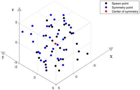
The convergence speed and accuracy of the butterfly algorithm are sensitive to the initial state. The initial population established by the pseudo-random number generator (PRNG) is usually not uniformly distributed in the high-dimensional space. The initial population optimization is achieved by using symmetric population amplification to increase the coverage area of the search space and retain the dominant population through the elite retention strategy. First, the initial population is established based on the pseudo-random number generator, and the population spatial distribution center is calculated. Then, the symmetric population is obtained through Equation 8 to achieve symmetric amplification of the population. The process of symmetric population amplification is shown in Figure 3. The black points are the initial population established by the pseudo-random number generator, the blue points are the symmetric population obtained by Equation 8, and the red point is the spatial center of the population distribution.

Figure 3

Figure 3. Schematic diagram of population symmetric amplification.

Population symmetric amplification:

$X_2=2*X_1-C,(8)$

where $X_1$ is the initial population of size n*dim created by the pseudo-random number generator, n is the number of populations, dim is the dimension of the population individuals, $C$ is the center of the population distribution space, and $X_2$ is the new population generated symmetrically by the center point.

When the current iteration ends, before starting the next iteration, two butterflies with the worst fitness in the current iteration population are processed for crossover variation (the number of butterflies in the population is 30; the reason for selecting 2 is because the selection of too many butterflies affects the convergence path of the algorithm, and it is more appropriate to select the number of individuals at approximately 1/10). Crossover processing is used for butterfly whose random generation number is less than the crossover probability $pc$, and all pairs of crossover methods are used after the crossover point. Uniform variation is used for butterfly whose random generation number is less than the variation probability $pm$, and the values of each dimension are replaced with random quantities that meet the boundary range. The iterative population after crossover and variation processing improves the diversity and provides the algorithm search a certain ability to jump out when it is caught in the local optimum problem.

2.2.2.2 Dynamic strategy

The values of sensory modality $c$ and power function exponential term $\mathit{\alpha }$ are all positive correlation parameters of adaptation degree. The larger the value taken in the early stage, the higher the fragrance, that is, the more clearly the optimal solution can be perceived by the rest of the global population individuals. The individual adaptation degree is adjusted by the global position update and local position search. The larger the step size, the easier it is to lock the optimal population range and thus speed up the convergence of the algorithm.

The size of the switching probability $p$-value determines the probability distribution of the global search and local search, and the control algorithm has a different emphasis on global and local search probabilities in different search periods. The first stage of the algorithm needs to quickly lock the region where the optimal solution is located and set a larger $p$-value for the first stage, focusing on global search; the later stage requires a deeper search in the region of the current better solution and set a smaller $p$-value for the later stage, focusing on local search.

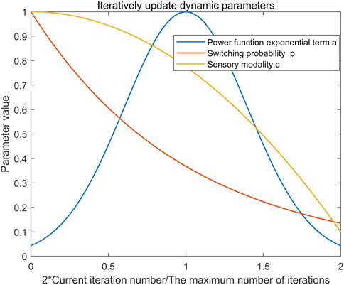
Combined with the demand for different search modes in different periods of the algorithm to improve the convergence speed and convergence accuracy, the dynamic change curves of sensory modality $c$, power function exponential term $\mathit{\alpha }$, and switching probability $p$ are constructed, as shown in Figure 4.

Figure 4

Figure 4. Algorithm search parameter dynamic adaptive trend.

Sensory modality $c$ dynamically updated with the iterative process as shown in Equation 9:

$c=-0.225{\left(\frac{2t}{N}\right)}^2+1.(9)$

Power exponent $\mathit{\alpha }$ that updates dynamically with the iterative process as shown in Equation 10:

$\alpha =e^{-\pi *{\left(\frac{2t}{N}-1\right)}^2}.(10)$

The switching probability $p$ that updates dynamically with the iterative process as shown in Equation 11:

$p=e^{-\frac{2t}{N}},(11)$

where $t$ is the current number of iterations and $N$ is the maximum number of iterations.

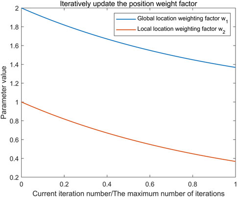
In order to meet the location update requirements of the algorithm to increase the global location update breadth in the early stage and the random search depth of the local location range in the later stage, the location update strategy for increasing the dynamic weight operator is constructed, and the overall trend of the dynamic update weight operator of the location is shown in Figure 5.

Figure 5

Figure 5. Dynamic trend of the location update weighting factor.

Global position update operator $w_1$ as shown in Equation 12:

$w_1=e^{-\frac{t}{N}}+1.(12)$

Local position update operator $w_2$ as shown in Equation 13:

$w_2=e^{-\frac{t}{N}}.(13)$

Global position update after the introduction of the weight operator as shown in Equation 14:

$x_i^{t+1}=w_1*x_i^t+\left(r^2*g^{*}-x_i^t\right)*f_i.(14)$

Local position update after the introduction of the weight operator as shown in Equation 15:

$x_i^{t+1}=w_2*x_i^t+\left(r^2*x_j^t-x_k^t\right)*f_i.(15)$

2.2.2.3 Algorithm flow

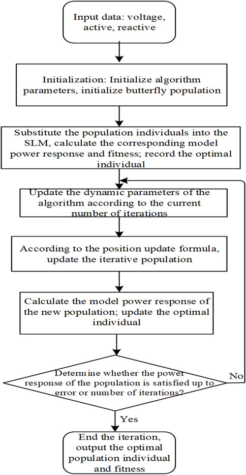
The initial population is optimized, and the disadvantaged population and other population optimization strategies are improved, combined with adaptive dynamic search parameters and a variable weight position update factor strategy to optimize the butterfly algorithm. The advantages of the two optimization strategies are combined to form a PODSBOA based on the population optimization and dynamic parameter strategy, and the complete flow of the algorithm is shown in Figure 6.

Step 1: The butterfly algorithm search parameters are initialized, the number of butterfly populations is set to $n$, the maximum number of iterations of the algorithm is set to $N$, the population boundary conditions [$L_b$, $U_b$], and the dimension of the optimization search problem dim.

Step 2: The initial butterfly population of size $n$*dim is generated by using random numbers according to the boundary conditions in the boundary range, and the initial population size is expanded to $2n$*dim by spatial symmetry.

Step 3: Fitness calculation—the fitness of butterflies in the expanded population is calculated according to the fitness criterion function.

Step 4: Population recovery—$n$ individuals with the best fitness are selected by an elite retention strategy and recorded as the recovery population, and the best individuals of the current recovery population are found and recorded.

Step 5: Disadvantaged population update—the two butterfly with the worst fitness are selected, and crossover and mutation operations are performed on them.

Step 6: Dynamic update of algorithm parameters—sensory modality $c$, power function exponential term $\mathit{\alpha }$, switching probability $p$, and position update operators $w_1$ and $w_2$ are updated according to the current number of iterations $t$.

Step 7: The current fragrance of each butterfly is calculated according to the updated parameters.

Step 8: Iterative optimization search—a random number between 0 and 1 is generated, denoted as rand. If the switching probability $p$ >rand, the position of the individual is updated globally; if the switching probability $p$ <rand, the position of the individual is updated locally.

Step 9: The global optimal value is calculated after individual updates.

Step 10: Out-of-bounds check—it is checked whether the updated individual is out of bounds, and the position of the new individual that is out of bounds is corrected.

Step 11: It is determined whether the current end condition of the iteration of the algorithm is satisfied. If the end condition is not satisfied, the algorithm turns to step 5 to continue the execution; conversely, the current optimal result is output, and the algorithm ends.

Figure 6

Figure 6. Flowchart of the PODSBOA.

3 Results

3.1 Synthesis load model identification process

3.1.1 Identification scheme

3.1.1.1 Identification criteria

The data used in the identification process are in the case of self-disturbance, including the data collected in the whole process of the load node before the disturbance, the disturbance process, and the gradual recovery to the steady state after the disturbance. The data type is the dynamic operation data of voltage and power.

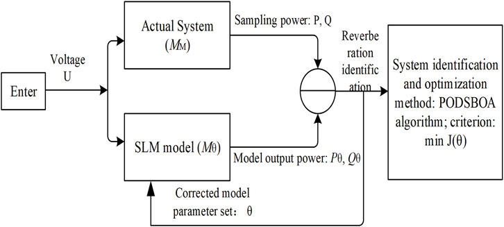
The identification criterion is to find the parameter group that can make the synthesis power response of the power function model and the motor model closest to the disturbance sampling data under the same voltage input. The parameter group that can achieve the optimal response is the parameter identification result. The dynamic model parameter identification criteria of the SLM are shown in Figure 7.

Figure 7

Figure 7. Dynamic model parameter identification criteria of the SLM.

3.1.1.2 Objective function

According to the output relationship of the SLM, it is known that according to the power composition of the model, the total load power is characterized by static load power $P_s$, $Q_s$, and motor load power $P_{im}$, $Q_{im}$, and the active and reactive power are identified simultaneously. The SLM identification objective function is shown in Equations 16, 17.

$\left\{\begin{array}{l}{J}_{\left({\theta }_{\sum P}\right)}=\sqrt{\left(\frac{{\displaystyle \sum _{i=1}^N}{\left(P_S+P_{im}-P\right)}^2}{N}\right)}\\ J_{\left({\theta }_{\sum Q}\right)}=\sqrt{\left(\frac{{\displaystyle \sum _{i=1}^N}{\left(Q_S+Q_{im}-Q\right)}^2}{N}\right)}\end{array}\right.,(16)$

$\left\{\begin{array}{l}J\left(\theta \right)=\sqrt{{J_{\left({\theta }_{\sum P}\right)}}^2+{J_{\left({\theta }_{\sum Q}\right)}}^2}\\ \epsilon =J\left(\theta \right)*N\end{array}\right.,(17)$

where $P_s$ and $Q_s$ are power responses of the power function model; $P_{im}$ and $Q_{im}$ are power responses of the motor model; $P$ and $Q$ are actual power data; $N$ is the number of sample data points; $J_{\left({\theta }_{\sum P}\right)}$ and $J_{\left({\theta }_{\sum Q}\right)}$ are model active and reactive power discrimination errors, respectively; $J\left(\theta \right)$ is the model synthesis identification error; and $\epsilon$ is the identification accuracy and is numerically equal to the absolute error accumulation sum of single point data.

3.1.1.3 Identification process

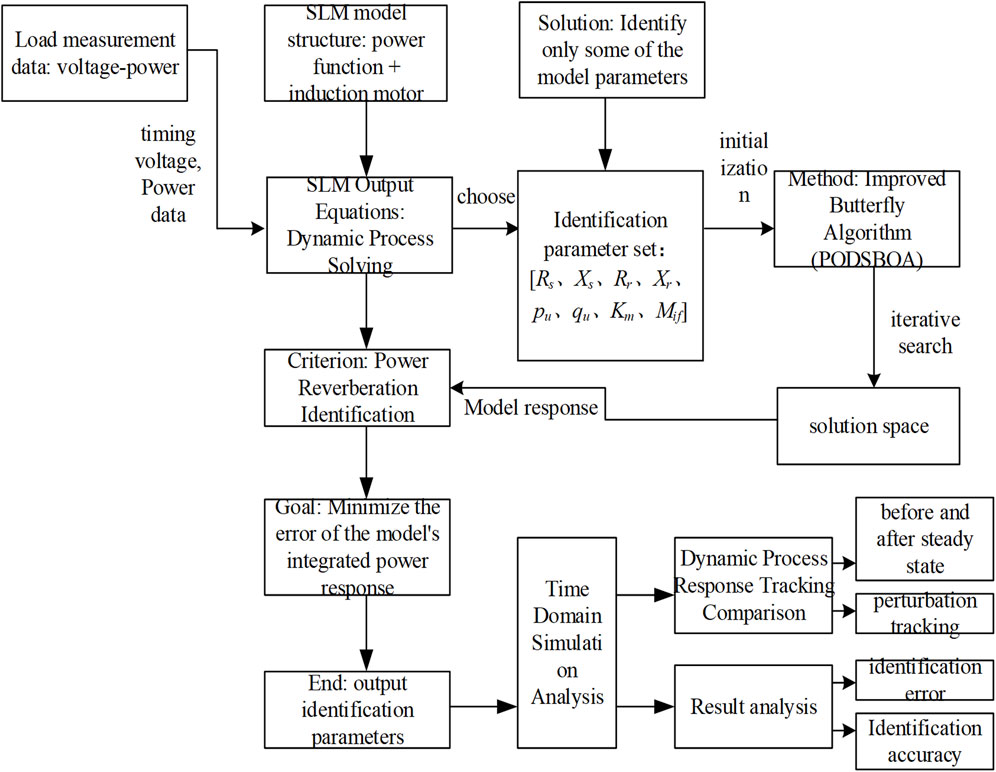
First, the motor parameters and voltage power data are input, and then the slip and transient potential are initialized according to the known parameters such as static model parameters, motor model parameters, dynamic and static load ratio, and motor load rate. Finally, the terminal current, terminal power, and total active and reactive power output of the model are solved. Based on the power response identification criterion, the minimum synthesis power response error of the model is taken as the goal, the parameter group to be identified is continuously modified by the PODSBOA, and the final identification result is output.

The dynamic load model adopts the SLM structure of motor load in parallel with static load, and the SLM parameters are identified by an intelligent optimization algorithm, in which the SLM identification process using the optimization algorithm is shown in Figure 8.

Figure 8

Figure 8. SLM dynamic model parameter identification scheme.

3.1.2 Dynamic model parameter identification process using the PODSBOA

The PODSBOA is used to complete the identification of the dynamic model parameters, and the specific steps of the PODSBOA for dynamic model parameter identification are shown in Figure 9. The insensitive parameters are set as typical parameters values, and only the important parameters of the remaining part are identified. The set of key parameters to be identified for the SLM is [$p_u$, $q_u$, $R_s$, $X_s$, $R_r$, $X_r$, $K_m$, and $M_{if}$].

Figure 9

Figure 9. Process of identifying the parameters of the dynamic model by the PODSBOA.

3.2 Result verification and performance comparison

3.2.1 Identification data source

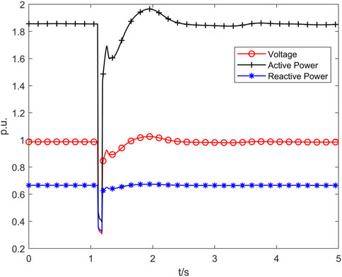
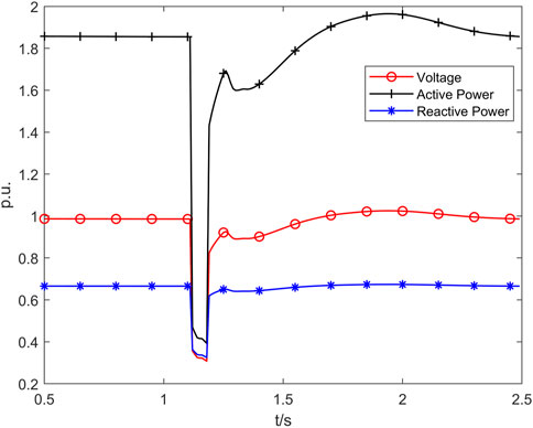
Dynamic model parameter identification uses the dynamic load characteristic data shown in Figure 10; a single-phase short-circuit fault occurs at 1.12 s, the data sampling time interval is 0.01 s, and the voltage starts to decrease when the fault occurs at 1.12 s and starts to recover at 1.20 s. The collected data types include voltage and active power, reactive power, and fault recording data lasting 5 s in total.

Figure 10

Figure 10. Sampling data of the disturbance fault recorder.

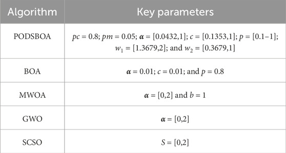
The simulation environment of the algorithm test experiment is as follows: the computer operating system is Windows 10, and the CPU is Intel@Core TM i5-6200U. The main frequency of the system is 2.30 GHz, the memory is 8.0 GB, and the simulation software version is MATLAB 2019a. The basic parameters of the five algorithms PODSBOA, BOA, modified whale optimization algorithm (MWOA) (Zhang and Chen 2018), gray wolf optimizer (GWO), and sand cat swarm optimization (SCSO) are the same. The population number is set to 30, and the maximum number of iterations is 500. The key parameters of the five algorithms PODSBOA, BOA, MWOA, GWO, and SCSO are set as shown in Table 3.

Table 3

Table 3. Key parameters of each algorithm.

In the PODSBOA, the power exponent $\mathit{\alpha }$ is a Gaussian kernel function varying with the number of iterations, the sensory modality $c$ is a parabolic function attenuating with the number of iterations, and the switching probability $p$ is a power function attenuating with the number of iterations. The global position update weight operator $w_1$ attenuates from 2.0 to 1.3679 with the number of iterations, and the local position update weight operator $w_2$ attenuates from 1.0 to 0.3679 with the number of iterations.

3.2.2 Identification process and results

The complete disturbance data lasting 5-s and the disturbance data from 0.5 s to 2.5-s are selected separately as the identification data for the iterative identification and optimization of the model parameters, as shown in Figures 10, 11. In the 2-s disturbance data recognition experiment, the data proportion of the steady-state process before disturbance and the process of recovery to the steady-state after the disturbance are reduced, and the data proportion of the disturbance process is increased, focusing on the tracking ability of the load model for the changes of the load characteristics during the disturbance.

Figure 11

Figure 11. Fault disturbance sampling data (0.5 s–2.5 s).

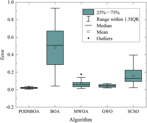
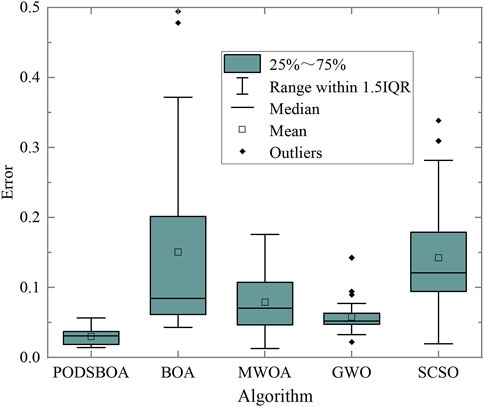
The PODSBOA, BOA, MWOA, GWO, and SCSO are used to identify the model parameters, and the identification results are shown in Tables 4, 5. The error is the single-point average absolute error of the synthesis power response of the model. In the experiment where disturbance data from 0.5 s to 2.5-s is selected as the identification data are shown in Figure 12A; the power response of SLM parameter identification is shown in Figures 12B, C, the iterative convergence process of the five algorithms is shown in Figure 12D, and the box and whisker plot diagrams of identification errors of each algorithm are shown in Figure 13. In the experiment of all 5-s disturbance data, the solution of the transient potential of the dynamically changing motor and the calculation results of the machine end current are shown in Figure 14A; the power response of SLM parameter identification is shown in Figures 14B, C, the iterative convergence process of the five algorithms is shown in Figure 14D, and the box and whisker plot diagrams of identification errors of each algorithm are shown in Figure 15. In order to prove the significance of the algorithms’ identification results, the Wilcoxon signed ranks test was performed on each algorithm, and the p-value results are shown in Table 5 (0.5 s–2.5 s) and Table 7 (0 s–5 s).

Table 4

Table 4. Parameter identification results of the dynamic load model (0.5 s–2.5 s).

Table 5

Table 5. p-value of the Wilcoxon signed rank test between each algorithm and the PODSBOA.

Figure 12

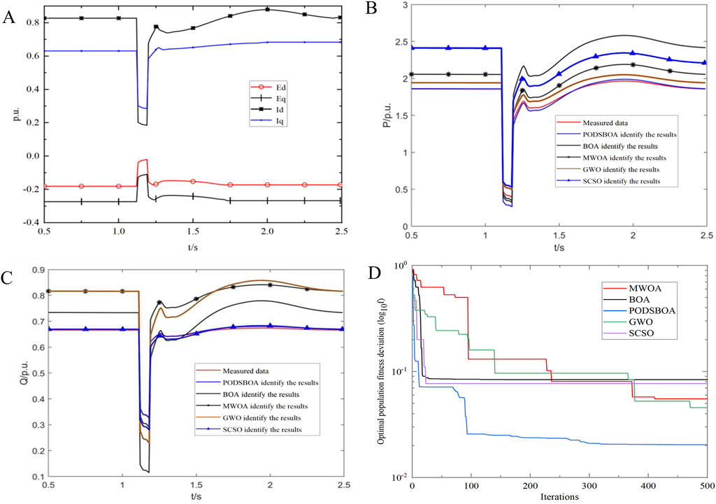
Figure 12. (A) Main process variables of motor model identification and calculation. (B) Active power response of SLM identification. (C) Reactive power response of SLM identification. (D) Iterative convergence curve (comparison of five algorithms).

Figure 13

Figure 13. Box and whisker plot diagrams of identification errors of each algorithm (0.5 s–2.5 s).

Figure 14

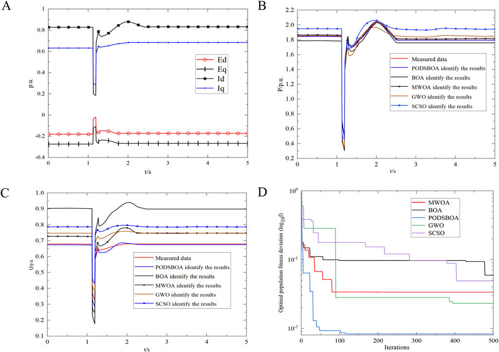
Figure 14. (A) Main process variables of motor model identification and calculation. (B) Active power response of SLM identification. (C) Reactive power response of SLM identification. (D) Iterative convergence curve (comparison of five algorithms).

Figure 15

Figure 15. Box and whisker plot diagrams of identification errors of each algorithm (0 s–5 s).

3.2.3 Analysis of the results

Based on the 2-s duration load data and 5-s duration load data for model parameter identification, by analyzing the results obtained by identifying load model parameters using the five algorithms, it can be concluded that

(1) According to Figures 12, 14D, by comparing the convergence curves, it can be found that the SLM identification results obtained based on the PODSBOA have the highest convergence accuracy compared to those obtained using the BOA, MWOA, GWO, and SCSO, and the model identification error based on the 2-s duration data is 0.02017, and the identification accuracy is 4.09, which is better than 4.6215 obtained using the mutational PSO with S-curve inertia weight (S-MPSO) (Shen 2013), Similarly, the model identification error based on the 5-s duration data is 0.01337, and the identification accuracy is 6.65, which is better than 6.6842 obtained using the S-MPSO, which illustrates the excellent effect of the PODSBOA proposed in this paper for load model parameter identification, and the dynamic model parameter identification scheme based on the PODSBOA to identify the key parameters of SLM: [$p_u$, $q_u$, $R_s$, $X_s$, $R_r$, $X_r$, $K_m$, $M_{if}$], realizes the refined identification of SLM parameters.

(2) According to Figures 12B, C, based on the power response of the model, the power response of the SLM identification model of the PODSBOA starts to decrease at 1.12 s, lasts 0.08 s, and then starts to recover and gradually returns to smooth operation from 1.2 to 2.0 s, which is consistent with the actual fault recording data situation and can accurately reflect the real level of the actual load, and realizes the fine identification of load model parameters, and from the box and whisker plot diagrams of identification errors of each algorithm in Figures 13, 15, it can be seen that the PODSBOA has the best robustness in the identification process of 2 and 5 s sampling data.

(3) Tables 4, 6 show that in the 2-s load data experiment, the convergence time of the PODSBOA is 12.048 s, which is lesser than that of MWOA and GWO and slightly larger than that of BOA and SCSO. The same is true in the experiment of 5 s load data, which is determined by the increased computational effort of the improved algorithm itself, and illustrates that the improved butterfly algorithm ensures faster convergence speed. Tables 5, 7 list the p-values of the PODSBOA and other algorithms at the 5% significance level. When p is less than 5%, it indicates that there is a significant difference between the two comparison algorithms, and when p is greater than 5%, it means that the difference between the two algorithms is not obvious. It can be seen that the p-values of the four comparison algorithms are all less than the significance level of 5%, which means that there is a significant difference between the PODSBOA and other algorithms, and the PODSBOA is statistically superior.

(4) Comparing the results of identification using load disturbance data of two pre- and post-steady-state processes with different time lengths, when the same identification method is used, the identification accuracy of the PODSBOA is 4.09 based on 2-s data, and the identification accuracy of the PODSBOA is 6.65 based on 5-s data. By appropriately increasing the proportion of the disturbance process in the total data and reducing the sampling time of the process data before and after steady state, the identification accuracy of the load model can be improved. This is because in the load model parameter identification, more attention is paid to the load change of the disturbance process. The data before and after steady state should not be selected too long to avoid interference with the disturbance data during the identification process.

Table 6

Table 6. Parameter identification results of the dynamic load model (0 s–5 s).

Table 7

Table 7. p-value of the Wilcoxon signed rank test between each algorithm and the PODSBOA.

4 Discussion

This paper proposes the improved butterfly algorithm by combining the basic population optimization and dynamic strategy optimization, which solves the SLM parameter identification problem, reduces the identification error of SLM parameters, and improves the accuracy and stability of the model parameter identification results. The model identification error of the proposed algorithm in 2 s load data is 0.02, which is better than the identification errors of BOA, MWOA, GWO and SCSO. Similarly, the model identification error of the algorithm proposed in this paper in 5 s load data is 0.013, which is also better than the identification errors of BOA, MWOA, GWO and SCSO, and the convergence speed is much higher than that of the improved algorithm MWOA. The identification situation is also consistent with the actual fault recording data, which shows that the proposed algorithm can accurately reflect the real level of the actual load and realize the fine identification of SLM parameters quickly and accurately. However, there are still shortcomings. The proposed improved algorithm is based on the number of iterations to adjust the dynamic parameters, and the next step is to consider combining fitness to further optimize the search mode of the algorithm. Due to the limitation of space, only the effect of dynamic load model parameter identification based on the perturbed data of single-phase grounded short-circuit fault type is explained, and the effect of model identification based on the perturbed data of the remaining fault cases is not explained. In the next step, a variety of identification studies can be carried out for different fault disturbances to further verify the generalization ability of the proposed method.

Data availability statement

The raw data supporting the conclusion of this article will be made available by the authors, without undue reservation.

Author contributions

ZW: conceptualization, investigation, methodology, and writing–review and editing. GY: data curation, formal analysis, methodology, visualization, and writing–review and editing. YR: formal analysis, validation, and writing–original draft. HW: formal analysis, visualization, and writing–original draft.

Funding

The author(s) declare financial support was received for the research, authorship, and/or publication of this article. This work was financially supported by Jiangxi Electric Power Company of State Grid. The funder was not involved in the study design, collection, analysis, interpretation of data, the writing of this article, or the decision to submit it for publication.

Conflict of interest

The authors declare that the research was conducted in the absence of any commercial or financial relationships that could be construed as a potential conflict of interest.

Publisher’s note

All claims expressed in this article are solely those of the authors and do not necessarily represent those of their affiliated organizations, or those of the publisher, the editors, and the reviewers. Any product that may be evaluated in this article, or claim that may be made by its manufacturer, is not guaranteed or endorsed by the publisher.

References

Arora, S., and Singh, S. (2019). Butterfly optimization algorithm: a novel approach for global optimization. Soft Comput. 23 (3), 715–734. doi:10.1007/s00500-018-3102-4

CrossRef Full Text | Google Scholar

Bacanin, N., Stoean, R., Zivkovic, M., Petrovic, A., Rashid, T. A., and Bezdan, T. (2021). Performance of a novel chaotic firefly algorithm with enhanced exploration for tackling global optimization problems: application for dropout regularization. Mathematics 9 (21), 2705. doi:10.3390/MATH9212705

CrossRef Full Text | Google Scholar

Bai, G., and Jing, P. (2015). Kinematic parameter identification of parallel manipulator based on improved particle swarm algorithm. Inf. Control 44 (5), 545–551. doi:10.13976/j.cnki.xk.2015.0545

CrossRef Full Text | Google Scholar

Bu, F., Ma, Z., Yuan, Y., and Wang, Z. (2020). WECC composite load model parameter identification using evolutionary deep reinforcement learning. IEEE Trans. Smart Grid 11 (99), 5407–5417. doi:10.1109/tsg.2020.3008730

CrossRef Full Text | Google Scholar

Chen, Y., Wu, H., Shen, Y., Meng, X., and Ju, P. (2022). A fast parameter identification method for composite load model based on jumping and steady-state points of measured data. IEEE Access 10, 97665–97676. doi:10.1109/ACCESS.2022.3206380

CrossRef Full Text | Google Scholar

Cheng, Y., and Ju, P. (2003). Measured dynamic load parameters and power network stability calculation. Electr. Power Autom. Equip. 23 (4), 19–21. doi:10.3969/j.issn.1006-6047.2003.04.005

CrossRef Full Text | Google Scholar

El-Shimy, M., Mostafa, N., Afandi, A. N., Sharaf, A. M., and Attia, M. A. (2018). Impact of load models on the static and dynamic performances of grid-connected wind power plants: a comparative analysis. Math. Comput. Simul. 149, 91–108. doi:10.1016/j.matcom.2018.02.003

CrossRef Full Text | Google Scholar

Jordehi, A. R., Javadi, M. S., and Catalão, J. P. (2020). “Dynamic economic load dispatch in isolated microgrids with particle swarm optimisation considering demand response,” in 2020 55th International Universities Power Engineering Conference (UPEC), Turin, Italy, 01-04 September 2020 (IEEE), 1–5. doi:10.1109/UPEC49904.2020.9209769

CrossRef Full Text | Google Scholar

Ju, P., Jin, Y., Chen, Q., Shao, Z., and Mao, C. (2010). Identifiability and identification of a synthesis load model. Sci. China Technol. Sci. 02, 461–468. doi:10.1007/s11431-009-0404-x

CrossRef Full Text | Google Scholar

Ju, P., Xie, H., and Chen, Q. (2007). Development trend of electric load modeling research. J. Automation Electr. Power Syst. 31 (2), 1–4. doi:10.3321/j.issn:1000-1026.2007.02.00

CrossRef Full Text | Google Scholar

Kang, P., Zhu, S., Wang, H., Fan, G., and Yang, G. (2021). Parameter identification of comprehensive load model with photovoltaic generation based on the IBOA algorithm. Renew. Energy Resour. 39 (11), 1541–1547. doi:10.13941/j.cnki.21-1469/tk.2021.11.018

CrossRef Full Text | Google Scholar

Kosterev, D. N., Taylor, C. W., and Mittelstadt, W. A. (1999). Model validation for the August 10, 1996 WSCC system outage. IEEE Trans. power Syst. 14 (3), 967–979. doi:10.1109/59.780909

CrossRef Full Text | Google Scholar

Ma, J., Han, D., He, R. M., Dong, Z. Y., and Hill, D. J. (2008). Reducing identified parameters of measurement-based composite load model. IEEE Trans. Power Syst. 23 (1), 76–83. doi:10.1109/TPWRS.2007.913206

CrossRef Full Text | Google Scholar

Mahdavi, M., Javadi, M. S., Wang, F., and Catalão, J. P. (2021). “Optimal modeling of load variations in distribution system reconfiguration,” in 2021 IEEE International Conference on Environment and Electrical Engineering and 2021 IEEE Industrial and Commercial Power Systems Europe (EEEIC/I&CPS Europe), Bari, Italy, 07-10 September 2021 (IEEE), 1–6. doi:10.1109/EEEIC/ICPSEurope51590.2021.9584545

CrossRef Full Text | Google Scholar

Shen, L. (2013). Research on parameter identification of power load model based on improved particle swarm optimization. China: Dalian Maritime University (Master thesis).

Google Scholar

Tang, Y., Zhang, H., Zhang, D., and Hou, J. (2009). A synthesis load model with distribution network for power transmission system simulation and its validation. IEEE Power and Energy Society General Meeting, 1–7.

Google Scholar

Wang, J., and Han, M. M. J. (2010). “A new identification strategy for improving convergence stability of load model parameters,” in International Conference on Electrical and Control Engineering, Wuhan, China, 25-27 June 2010 (IEEE), 145–148.

Google Scholar

Yuan, H., Dai, H., Wei, X., and Ming, P. (2021). Internal polarization process revelation of electrochemical impedance spectroscopy of proton exchange membrane fuel cell by an impedance dimension model and distribution of relaxation times. Chem. Eng. J. 418, 129358. doi:10.1016/J.CEJ.2021.129358

CrossRef Full Text | Google Scholar

Zad, B. B., Lobry, J., and Vallée, F. (2017). “Impacts of the load and line inaccurate models on the voltage control problem of the MV distribution systems,” in 52nd International Universities Power Engineering Conference (UPEC), Heraklion, Greece, 28-31 August 2017 (IEEE), 1–6. doi:10.1109/UPEC.2017.8231928

CrossRef Full Text | Google Scholar

Zhang, Y., and Chen, F. (2018). A modified whale optimization algorithm. Comput. Eng. 44 (03), 208–213+219. doi:10.3969/j.issn.1000-3428.2018.03.035

CrossRef Full Text | Google Scholar

Zhao, J., Ju, P., Shi, J., and Qin, C. (2020). Review and prospects for load modeling of power system. J. Hohai Univ. Sci. 48 (1), 87–94. doi:10.3876/j.issn.10001980.2020.01.013

CrossRef Full Text | Google Scholar

Zhou, L., Peng, Z., Deng, C., Qi, X., and Li, P. (2018). A generalized synthesis load model considering network parameters and all-vanadium redox flow battery. Prot. Control Mod. Power Syst. 3, 32–13. doi:10.1186/s41601-018-0105-1

CrossRef Full Text | Google Scholar

Zivkovic, M., Tair, M., Venkatachalam, K., Bacanin, N., Hubálovský, Š., and Trojovský, P. (2022). Novel hybrid firefly algorithm: an application to enhance XGBoost tuning for intrusion detection classification. PeerJ. Comput. Sci. 8, e956. doi:10.7717/PEERJ-CS.956

CrossRef Full Text | Google Scholar