Study on mining wind information for identifying potential offshore wind farms using deep learning

The global energy demand is increasing due to climate changes and carbon usages. Accumulating evidences showed energy sources using offshore wind from the sea can be added to increase our consumption capacity in long term. In addition, building offshore wind farms can also be environmentally advantageous compared to onshore farms. The assessment of wind energy resources is crucial for the site selection of wind farms. Currently, short-term wind forecast models have been developed to predict the wind power generation. However, methods are needed to improve the forecasting accuracy for ever-changing weather data. So, we try to use deep learning methods to predict long-term wind energy for identifying potential offshore wind farms. The experimental results indicate that PredRNN++ prediction model designed from the spatiotemporal perspective is feasible to evaluate long-term wind energy resources and has better performance than traditional LSTM.

1 Introduction

In the past centuries, fossil energy was the main source of energy for mankind. While enjoying the high-quality life brought by the advancements of fossil energy, it also brings a series of consequences such as resource depletion, environmental degradation and climate changes. In particular to climate changes, our planet’s average surface temperature has risen about 0.99°C from the late 19th century (Data source: NASA’s Goddard Institute for Space Studies). In addition, a change driven largely by an increased carbon dioxide and other human-made emissions into the atmosphere have been observed. Due to the increase of human activities since the industrial revolution, the current global warming trend is particularly significant (Doughty, 2013). Therefore, researching to meet global energy demands can bring enormous opportunities to human society and the energy industry (BUSINESS WIRE, 2017).

According to the latest assessment of global energy consumption by the International Energy Agency (IEA), global energy demand is growing at the fastest rate in a decade, which is an outstanding performance driven by a strong global economy. With the rapid growth of energy consumption, renewable energy (including solar, wind and hydro power) is the fastest growing energy source between 2018 and 2050 (S&P Global Market Intelligence, 2019). Among these fastest-growing energy sources, wind energy has become an important source of zero-carbon power, which is inseparable from the sharp decline in wind turbine costs and increasing installed capacity. The global wind energy distribution, as shown in Figure 1, illustrated there is huge potential for wind energy resource over the water (Possner and Caldeira, 2017). The evidence showed the offshore wind speed is much higher than onshore wind speed, and the ocean area is also much larger than the land area. Such aligns with the recent evidence to utilize offshore wind to increase the capacity for the repository of energy (Rusu, 2020).

Figure 1

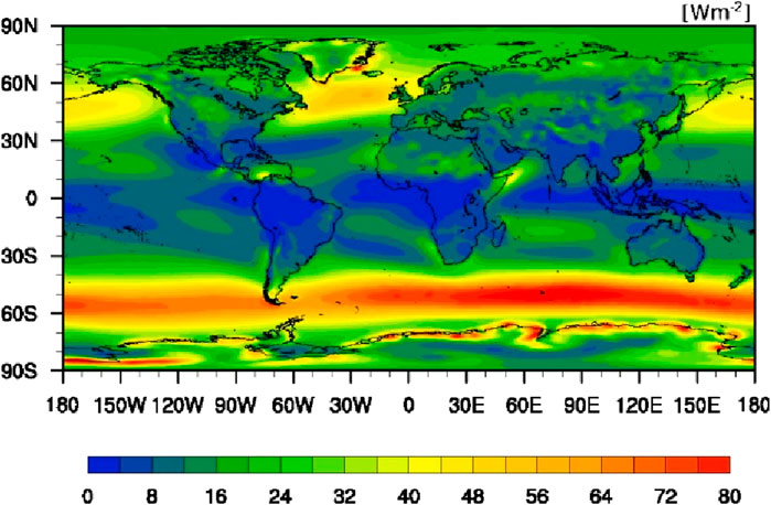
Figure 1. Global wind energy distribution.

From 2010 to 2018, the global offshore wind power market grew by nearly 30% annually, thanks to rapid technological improvements. In the next 5 years, about 150 new offshore wind power projects are planned to be accomplished, which indicates that offshore wind power is playing an increasingly significant role in power supply. If the world’s optimum offshore wind farm site is completed, it can exceed the current global electricity consumption demand. Although offshore wind energy has the advantages of clean, renewable, zero-carbon, etc., there are still great difficulties in the utilization of offshore wind energy, especially for the construction of offshore wind farm. Once these constraints are broken, offshore wind power will greatly alleviate the global energy crisis and climate problems. Especially for the densely populated and energy demanding Asian regions, such as China, South Korea and Hong Kong, the zero-carbon power generation technology of offshore wind power is taken as the key planning project in the future to reduce greenhouse gas emissions (FINANCIAL TIMES, 2018).

However, the wind as energy supply of offshore wind farm is unstable and uncontrolled. So, how to control turbines and predict the instability of wind power in advance has become an urgent problem for wind farms. In recent development, machine learning and deep learning in artificial intelligence technology supports the great progress of prediction methods. It can be found that from the above examples and related research literatures that the great majority of the current wind power forecasting is based on a very short-term prediction analysis (Heinermann and Kramer, 2016; Khan et al., 2019; Optis and Perr-Sauer, 2019). Usually wind power or wind speed can only be predicted for the next few days or weeks. But the studies for long-term wind energy prediction and assessment are scarce. In fact, the accurate and effective assessment of wind energy resources is of great significance to the study of large-scale wind power grid connection and demonstrating the feasibility of wind power project construction. It is the basic work of wind farm construction especially for the offshore wind farm.

The current assessment of offshore wind energy resources is generally carried out in the history of 1–30 years, and the operation period of offshore wind farms can reach more than 20 years at present, so the assessment of offshore wind farm site selection should be more concerned about wind energy potential in the next few decades. Besides, the accuracy of the offshore wind energy potential assessment results is directly related to the risks and profits of offshore wind farm investment. So, the first thing to do in building offshore wind farms is through the meteorological, geographic conditions and other aspects of comprehensive investigation to select the areas with rich wind energy resources. Currently, the classification and assessment methods for in offshore wind energy potential assessments are not uniform and difficult to quantify. The uncertain factors of wind energy resource assessment have not be classified and scientific enough, reasonable and operable assessment methods should be proposed. From the perspective of prediction methods, wind power prediction methods include: physical model method, statistical model method, machine learning method, and deep learning method, etc. The physical modeling method mainly relies on numerical weather prediction (NWP) to determine meteorological information for future periods. This method does not rely on the accumulation of historical data and can make predictions through high-precision numerical weather forecasting. It is suitable for short-term forecasting and the prediction model when there is sufficient meteorological geographic location data. The statistical modeling approach, grounded in statistics, integrates NWP with historical wind power data and employs fitting techniques to establish an input-output mapping, ultimately achieving the objective of wind power prediction. Traditional statistical models can capture linear relationships well, but perform poorly in non-linear relationships. Due to the wind power prediction is a highly nonlinear problem relying on variations in meteorological data, the predictability of features is harnessed to construct a model during input-output mapping, thereby enabling the prediction of wind power. Compared to traditional statistical methods, machine learning methods can effectively predict nonlinear time series data with significantly improved accuracy. The model performs well with small sample data, but has certain limitations when dealing with large amounts of data. On the basis of machine learning, deep learning methods have been further proposed, which can better process time series and spatial series predictions of large amounts of data. A LSTM-CNN joint model is proposed for predicting the wind power of multiple wind turbines to provide accurate power scheduling (Chen et al., 2021). Wind power prediction based on WT-BiGRU-attention-TCN model using deep learning methods provides a new solution to high-precision forecasting of wind power generation (Chi and Yang, 2023). And the digital twin of wind farms via physics-informed deep learning is developed to achieve the accurate in situ full field prediction including wind farm assessment, monitoring, power forecasting and scheduling (Zhang and Zhao, 2023). Learning from the experience of wind power prediction, we can also try to introduce machine learning and deep learning into the assessment of offshore wind energy resources to predict the offshore wind speed to evaluate the offshore wind energy potential.

In order to make more rational and efficient use of offshore wind energy resources and maximize the economic benefits of offshore wind farms and shorten its payback period of investment, optimize the offshore wind farm site selection from a long-term point of view is very necessary. Therefore, using deep learning methods to improve the scientific and accurate estimation of wind energy potential and predict its spatial distribution is a very worthwhile study for wind power development.

2 Key parameters and data

As for the potential prediction of offshore wind energy, we mainly consider the wind speed and wind energy density as the key parameters to be measured. Wind energy density, also known as wind power density, is the wind energy that the airflow passes through the unit cross-section area vertically in unit time, and the unit is watt per square meter. It is the most convenient and valuable quantity for describing the wind potential of a place. Wind energy density is directly proportional to the third power of wind speed and air density. The calculation formula of wind energy density is shown in Eq. 1.

$\omega =\frac{1}{2}\rho {\upsilon }^3(1)$

$\omega$ express wind energy density (w/m²), ρ express air density (kg/m³), $\upsilon$ express wind speed (m/s).

Additionally, the value of air density depends on temperature and altitude. The formula is shown in Eq. 2.

$\rho =\left(353.05/T\right)\mathit{exp}-0.034\left(\mathrm{z}/T\right)(2)$

$T$ in the above formula is the thermodynamic temperature scale (Kelvin temperature scale or absolute temperature scale), and $\mathrm{z}$ is the altitude of the wind turbine hub (m).

This calculation method can also be used for offshore wind energy potential assessment. After identifying the key parameters, we need to obtain accurate and reliable meteorological data. In this paper, we have chosen the data provided by the ECMWF as the data source. The meteorological dataset of the ECMWF is abundant and can be selected and downloaded easily. With rich data, the assessment of offshore wind energy potential has more reference value. Moreover, we have chosen the dataset “ERA5 monthly averaged data on single levels from 1979 to present” which is downloaded from the Climate Data Store (CDS) was launched online by the Copernicus Climate Change Service (C3S) operated by the ECMWF. The dataset is mostly derived from the six-hourly ERA-Interim reanalysis dataset by bias adjusting against observations using different methods. Data are then aggregated on daily, monthly, seasonal, and annual averages.

According to the research content and the above key parameters, we select the variables, shown in Table 1, that we need to use from the dataset. On the basis of the latest statistics abroad, the rotating diameter of large-scale wind turbine blades (that is, the range swept by the front blades) was nearly 100 m in 2014. Therefore, we select an existing offshore wind turbine with a general height of 100 m to evaluate the wind energy resources and because wind energy can only be transformed from the airflow passing through the unit cross-section area vertically. So, we need to calculate the horizontal speed of air moving, which is the u component of wind. There is no air density parameter for the atmosphere in the dataset, so we need to calculate the air density from the temperature. The temperature available in the dataset is that of air at 2 m above the sea surface and needs to later be revised into 100 m’s temperature of air. As for the ocean parameter, we can get the parameters of air density and wind speed directly from the dataset.

Table 1

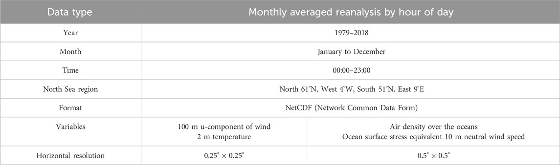
Table 1. Dataset of the key parameters.

In the geographical scope of the study, the North Sea of Europe as the main object of offshore wind resource assessment is quite suitable because the development of offshore wind power in Europe is more advanced and large-scale. The geographical conditions of the North Sea are also highly suitable for the construction of wind farms. By 2019, the cumulative installed capacity of offshore wind power in the North Sea had reached 16,908 MW, accounting for 77% of the total offshore wind power in Europe (WindEurope, 2020). There are many offshore wind farms under planning and construction. Therefore, the potential assessment of offshore wind energy resources in the North Sea area has important reference value.

The data we used in this dataset are of monthly averaged reanalysis by hour of day from 1979 to 2018, with s total of 11,520 (24 h × 12 months × 40 years) time points of sub-datasets for each variable. The geographical range is 51°N–61°N, 4°W–9°E, covering the entire area of the North Sea. And the data have been regridded to a regular latitude–longitude grid of 0.25° for the reanalysis of the variables for atmosphere and 0.5° for ocean waves. Therefore, each sub-dataset contains 2,080 (40 × 52) parameters of atmosphere and 1,040 (20 × 26) parameters of ocean waves. The dataset can be regarded as a series of image text composed of two-dimensional arrays; see Figures 2, 3.

Figure 2

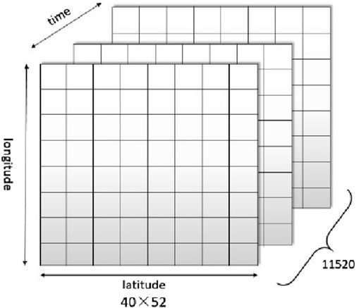
Figure 2. Data set of the atmosphere.

Figure 3

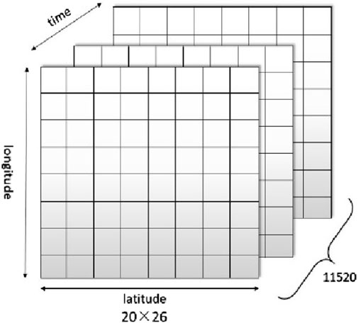
Figure 3. Data set of ocean surface.

Of note is that the wind speed in the dataset is that at 100 m altitude, but the temperature is at 2 m. Therefore, we need to correct the temperature to 100 m so that we can calculate the air density using Formula 2. According to the empirical formula, for every 100 m above sea level, the temperature drops 0.6°. So, the temperature at 100 m is 2 m temperature subtract 0.588 K (100–2)*0.6). The modified air density formula is shown in Eq. 3.

${\rho }_{100m}=\left(353.05/\left(T_{2m}-0.588\right)\right)\mathit{exp}-0.034\left(z/\left(T_{2m}-0.588\right)\right)(3)$

Regarding data format, NetCDF was developed by the Unidata project scientists of the University Corporation for Atmospheric Research (UCAR), aiming at the characteristics of scientific data. NetCDF format data are widely used in atmospheric science, hydrology, oceanography, geophysics, and many other fields. Mathematically, the data stored in NetCDF comprise a single valued function with multiple independent variables. In the function f (x, y, z…) = value, the independent variables x, y, and z of the function are called “dimension” or “axis” in NetCDF, and the value of function in NetCDF is called “variables.” However, the NetCDF file cannot be directly read by computer programming language. So, we need to write a program to convert NetCDF format data into CSV format, which stores data as plain text for subsequent input model processing.

3 Methodology–deep learning

3.1 Prediction models

In the process of deep learning development, people have established different types of neural networks with their own characteristics through continuous innovation and optimization, such as convolutional neural networks (CNN), generative adversarial networks (GAN), recurrent neural networks (RNN), deep belief networks (DBN), and so on (Pouyanfar et al., 2018). Among them, CNN and RNN are the most widely used at this stage. They constitute the basis of most of the pre-training models in deep learning.

The building block of CNN is a filter, called kernels. Kernel function is used to extract correct and related features from input data by convolution. The convolution of the image with filters generate the feature map to capture spatial features from the image (Krizhevsky et al., 2017). Therefore, CNN is often used in image classification, recognition, and video processing projects. While the RNN established a recurrent connection in the state to state transfer. Therefore, the chain structure of RNN successfully solves the problem of time sequence prediction and has been widely used in audio recognition, machine translation and other sequence data (Mandic and Chambers, 2001).

Although RNN can solve the time sequence problem, it also has some deficiencies like gradient explosions and vanishing gradient problems. To address the fact that the classical RNN cannot deal with the long-term memory problem, an LSTM networks model is proposed (Yu et al., 2019). LSTM establishes a long-term delay mechanism on the basis of RNN, which can avoid gradient vanishing or explosion problems by keeping a continuous error in the memory unit. Therefore, LSTM is a more suitable neural network for our wind energy potential prediction compared with RNN.

When evaluating the potential of wind energy resources, we should not only pay attention to the changes in the time dimension but also the spatial distribution. Therefore, Combined with the excellent performance of CNN in spatial feature extraction, ConvLSTM network was proposed in 2015 (Shi et al., 2015). ConvLSTM is equivalent to using a convolution operation instead of the fully connected method used as input to the state to state transfer process.

However, in ConvLSTM the time dimensions are independent of each other. To solve this problem, the team from Tsinghua University introduced a new building block called ST-LSTM in 2017 (Wang et al., 2017). It is equivalent to Adding an M state (the state of spatiotemporal memory) to the original LSTM. In this way, the drawback of ConvLSTM is solved.

Although the ST-LSTM already has a very good performance, some problems remain, such as the recursion depth and the gradient vanishing. Therefore, further improvement is made to put forward PredRNN++ in 2018 (Wang et al., 2018), which is the model we choose to use. Compared with ST-LSTM, the difference lies in the change of the cell from ST-LSTM to Causal LSTM and the addition of the gradient highway unit (GHU) structure between the first and second stack structures. The input of the GHU is the output of the current lower layer and the input of the previous time. It is similar to get the two inputs go through an update gate in GRU (Gate Recurrent Unit) (Dey and Salem, 2017). Therefore, the GHU connects the input of the current time and the previous time. The result of adding this new unit is that the gradient is no longer a strand of line propagation, but can directly spread between the first layer and the second layer. In other words, the propagation distance is shortened. And the network will not be as deep as before, which can effectively solve the problem of gradient vanishing.

3.2 Experiments

After the comparison and analysis of the above prediction models, we choose to bring our dataset into PredRNN++ (the model with the best performance of those above) for training. We use TensorFlow 2.0, which is more efficient and easy to deploy, as a framework to build, train, and validate the models (Singh and Manure, 2019). To take into account the accuracy of the prediction results and the training speed, we build the neural network model into five layers, which are composed of four causal LSTMs and one GHU. The GHU is set between the first and second layers. The structure is shown in Figure 4.

Figure 4

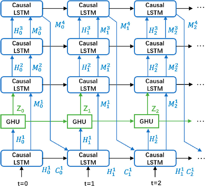
Figure 4. The structure of PredRNN++ model.

All kernel filter sizes in the model are set to 3, and the Adam optimization algorithm was used in the training process (Wang and Wang, 2020). As for the setting of the other hyper parameters, such as the learning rate or step size factor, it controls the update ratio of the weights. A larger value (such as 0.3) will have faster initial learning before the learning rate is updated, while a smaller value (such as 0.00001) will make the training converge to better performance. So, we set 0.001 as the initial learning rate. As for the objective function, we use the L1 + L2 loss to simultaneously enhance the sharpness and the smoothness of the generated frames. The L1and L2 are shown inEqs. 4, 5. As for the performance measurement of the model, we use the mean squared error (MSE) most commonly used in regression problems as the loss function to measure the accuracy of the prediction results. The calculation formula of the MSE is shown in Eq. 6, where t_i is the true value, and p_i is the predicted value.

$L1={\displaystyle {\sum }_{i=1}^n}\left|y_i-f\left(x_i\right)\right|(4)$

$L2={\displaystyle {\sum }_{i=1}^n}{\left(y_i-f\left(x_i\right)\right)}^2(5)$

$MSE=\frac{1}{N}{\displaystyle {\sum }_{i=1}^N}{\left(t_i-p_i\right)}^2(6)$

On the division of datasets, we divided 11,520 time sequence samples into a training set and a test set according to the ratio of 9:1. As the change of wind speed is seasonal, we divide the data samples according to the time series of 1 year. Therefore, the training set is divided into 36 batches of 288 each, and the test set is divided into 4 batches of 288 each. All these batches are brought into the model for iterative training. Finally, 40 years of wind energy data were brought into the optimized model, which was used to predict the wind energy in the next 20 years which is the average operating period of an offshore wind farm and visualize the data to create an average wind energy density map of the North Sea in the next 20 years.

At the same time, we set up a typical LSTM model also using TensorFlow and the same dataset to compare with the prediction results of the PredRNN++.

4 Results and discussions

4.1 Results

We bring the 100 m u-component of the wind energy density dataset calculated by wind speed and temperature, and ocean surface stress equivalent 10 m neutral wind energy density dataset calculated by wind speed and air density into PredRNN++ and LSTM models, respectively, for training and testing.

The results are shown in Figures 5, 6 above. It can be seen from the figure that the MSE of PredRNN++ and LSTM are very close at the beginning of the training process. The MSE of LSTM in wind speed prediction is even higher. With the increase of time steps, the MSE of the two models are constantly improving, and the MSE of PredRNN++ being smaller than that of LSTM. This illustrates that the PredRNN++ model considering spatial characteristics has more accuracy results for wind energy density prediction in a given region than the LSTM model which only considers the time sequence. Moreover, we can see that with the extension of the time steps PredRNN++ performs much better than LSTM. This is due to the fact that the GHU layer in PredRNN++ can effectively transfer the gradient in a very deep feedforward network and prevent the rapid vanishing of the long-term gradient. Therefore, the performance of PredRNN++ is more suited to long-term prediction.

Figure 5

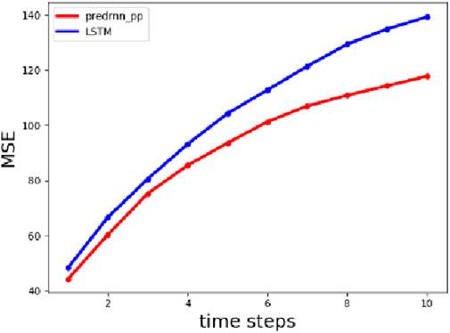
Figure 5. The prediction result of 100 m u-component wind energy density.

Figure 6

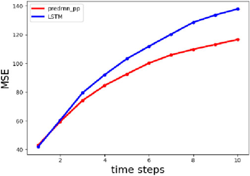
Figure 6. The prediction result of ocean surface stress equivalent 10 m neutral wind energy density.

Figure 7 is a map of wind energy density at 100 m altitude horizontal direction for the next 20 years (2020–2039) predicted by PredRNN++. The lighter the color, the greater the wind energy density like the yellow area. And the darker the color, the lower the wind energy density like the dark blue area. The wind energy density in the central part of the North Sea is relatively high, which is suitable for the construction of large-scale offshore wind farms. The highest wind energy density is around 57.5 °N and 8°E, which can reach 449.02 W/m2. And Figure 8 is a map of wind energy density at 10 m above ocean surface for the next 20 years (2020–2039) predicted by PredRNN++. The white area on the map represents the land, the lighter the same color, the higher the wind energy density. In the north central part of the North Sea, the wind energy density is high, the highest wind energy density is up to 839.45 W/m2. Because the wind speed measured 10 m above the sea surface is the natural wind speed, it is higher than the wind speed at 100 m of the atmosphere only considering u-component, and the wind energy density is higher.

Figure 7

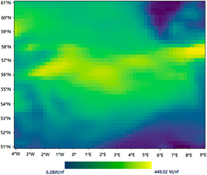
Figure 7. Average wind energy density over the next 20 years at 100 m

Figure 8

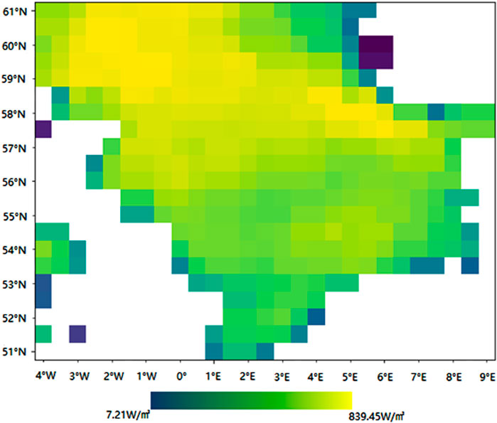
Figure 8. Average wind energy density over the next 20 years at 10 m above ocean surface.

Combining the results of the atmosphere condition and ocean surface condition, we can see that if you choose to build a large-scale offshore wind farm in the future, it is more appropriate to choose an area with a higher wind energy density at an altitude of 100 m in the atmosphere. If you choose to build an offshore wind farm that integrates wind and wave energy, it is more rational to choose an area with a higher wind energy density 10 m above the sea surface, since the area with higher wind energy also has greater wave energy.

4.2 Discussions

In future research, the accuracy rate of this model can be further improved with more data. And the prediction model can be further optimized. We can further improve the PredRNN++ model by combining it with other machine learning methods. For example, using the machine learning model XGBoost to extract corresponding temporal features, and using a CNN model to fuse temporal features into sea surface temperature data, and extracting spatial dependencies between the fused sea surface temperature data. On this basis, the PredRNN++ model was used to integrate spatiotemporal dependencies into the data sequence, avoiding the problem of gradient vanishing (Du et al., 2022).has used this method achieved better experimental results than the PredRNN++model in predicting sea surface temperature. With the latest advances in graph neural networks (GNNs), time series analysis methods based on GNNs have significantly increased (Jin et al., 2023). These methods can explicitly model the relationship between time series and variables, while other traditional deep neural network-based methods are difficult to achieve. Many time series data have characteristics in time and space, and different variables in the series capture information about different locations (spaces), which means it not only contains temporal information but also spatial relationships. So, GNN can play an important role in wind speed and power prediction, capturing the complex spatiotemporal dynamics of wind speed patterns, providing accurate predictions, and helping to effectively manage wind energy resources.

We can also add marine-related factors near the sea surface, such as the significant height of wind waves and mean wave period as variables put into the model. The model can also be applied to satellite weather maps for weather and climate prediction, which may achieve better results than a two-dimensional matrix dataset. Additionally, it is possible to consider extending this prediction model to the assessment of wind energy resources in onshore wind farms. Further extending the application scenarios, this wind power prediction model can also be applied in buildings equipped with wind and photovoltaic distributed power sources (Li et al., 2024; Ding et al., 2024).

5 Conclusion

Based on the results and discussions presented above, the conclusions are obtained as below:

(1) It is feasible to use deep learning to predict and evaluate long-term wind energy resources, especially with the PredRNN++ model.

(2) PredRNN++ prediction model designed from the spatiotemporal perspective, which has better performance than a traditional LSTM.

(3) We can use the predicted wind energy map for the next 20 years as a reference to select the location of the wind farm.

Data availability statement

The original contributions presented in the study are included in the article/Supplementary Material, further inquiries can be directed to the corresponding author.

Author contributions

JZ: Writing–original draft, Writing–review and editing. TZ: Writing–original draft, Writing–review and editing. YL: Writing–original draft, Writing–review and editing. XB: Writing–original draft, Writing–review and editing. LC: Writing–original draft, Writing–review and editing.

Funding

The author(s) declare that no financial support was received for the research, authorship, and/or publication of this article.

Conflict of interest

Author TZ was employed by Shanghai Zhongyuan Network Technology Co., Ltd.

The remaining authors declare that the research was conducted in the absence of any commercial or financial relationships that could be construed as a potential conflict of interest.

Publisher’s note

All claims expressed in this article are solely those of the authors and do not necessarily represent those of their affiliated organizations, or those of the publisher, the editors and the reviewers. Any product that may be evaluated in this article, or claim that may be made by its manufacturer, is not guaranteed or endorsed by the publisher.

References

BUSINESS WIRE (2017). Well intervention market by services. Available at: https://www.businesswire.com/news/home/20170426005652/en/Well-Intervention-Market-by-Services-Application-Region March 15, 2018.

Google Scholar

Chen, X., Zhang, X., Dong, Mi, Huang, L., Guo, Y., and He, S. (2021). Deep learning-based prediction of wind power for multi-turbines in a wind farm. Front. Energy Res. 9, 723775. doi:10.3389/fenrg.2021.723775

CrossRef Full Text | Google Scholar

Chi, D., and Yang, C. (2023). Wind power prediction based on WT-BiGRU-attention-TCN model. Front. Energy Res. 11, 1156007. doi:10.3389/fenrg.2023.1156007

CrossRef Full Text | Google Scholar

Dey, R., and Salem, F. M. (2017). “Gate-variants of Gated Recurrent Unit (GRU) neural networks,” in IEEE 60th International Midwest Symposium on Circuits and Systems (MWSCAS), Boston, MA, 1597–1600. doi:10.1109/MWSCAS.2017.8053243

CrossRef Full Text | Google Scholar

Ding, B., Li, Z., Li, Z., Xue, Y., Chang, X., Su, J., et al. (2024). A CCP-based distributed cooperative operation strategy for multi-agent energy systems integrated with wind, solar, and buildings. Appl. Energy 365, 123275. doi:10.1016/j.apenergy.2024.123275

CrossRef Full Text | Google Scholar

Doughty, C. E. (2013). Preindustrial human impacts on global and regional environment. Annu. Rev. Environ. Resour. 38, 503–527. doi:10.1146/annurev-environ-032012-095147

CrossRef Full Text | Google Scholar

Du, Y. F., Wu, X. F., and Qiao, B. Y. (2022). Sea surface temperature prediction based on XGBoost-PredRNN++. Comput. Syst. Appl. 31 (10), 236–244. (in Chinese).

Google Scholar

FINANCIAL TIMES (2018). Offshore wind to rise 20-fold in Asia but solar slows: report. ■■■: ■■■. Available at: https://www.ft.com/content (Accessed October 24, 2018).

Google Scholar

Heinermann, J., and Kramer, O. (2016). Machine learning ensembles for wind power prediction. Renew. Energy 89, 671–679. doi:10.1016/j.renene.2015.11.073

CrossRef Full Text | Google Scholar

Jin, M., Koh, H., Wen, Q., Zambon, D., Alippi, C., Webb, G. I., et al. (2023). A survey on graph neural networks for time series: forecasting, classification, imputation, and anomaly detection. China: ArXiv.

Google Scholar

Khan, M., Liu, T., and Ullah, F. (2019). A new hybrid approach to forecast wind power for large scale wind turbine data using deep learning with TensorFlow framework and principal component analysis. Energies 12 (12), 2229. doi:10.3390/en12122229

CrossRef Full Text | Google Scholar

Krizhevsky, A., Sutskever, I., and Hinton, G. E. (2017). ImageNet classification with deep convolutional neural networks. Commun. ACM 60 (6), 84–90. doi:10.1145/3065386

CrossRef Full Text | Google Scholar

Li, Z., Su, S., Jin, X., Xia, M., Chen, Q., and Yamashita, K. (2024). Stochastic and distributed optimal energy management of active distribution networks within integrated office buildings. CSEE J. Power Energy Syst. 10 (2), 504–517.

Google Scholar

Mandic, D. P., and Chambers, J. (2001). Recurrent neural networks for prediction: learning algorithms, architectures and stability. USA: John Wiley and Sons, Inc.

Google Scholar

Optis, M., and Perr-Sauer, J. (2019). The importance of atmospheric turbulence and stability in machine-learning models of wind farm power production. Renew. Sustain. Energy Rev. 112, 27–41. doi:10.1016/j.rser.2019.05.031

CrossRef Full Text | Google Scholar

Possner, A., and Caldeira, K. (2017). Geophysical potential for wind energy over the open oceans. Proc. Natl. Acad. Sci. 114 (43), 11338–11343. doi:10.1073/pnas.1705710114

PubMed Abstract | CrossRef Full Text | Google Scholar

Pouyanfar, S., Sadiq, S., Yan, Y., Tian, H., Tao, Y., Reyes, M. P., et al. (2018). A survey on deep learning: algorithms, techniques, and applications. ACM Comput. Surv. (CSUR) 51 (5), 1–36. doi:10.1145/3234150

CrossRef Full Text | Google Scholar

Rusu, E. (2020). An evaluation of the wind energy dynamics in the Baltic Sea, past and future projections. Renew. Energy 160, 350–362. doi:10.1016/j.renene.2020.06.152

CrossRef Full Text | Google Scholar

Shi, X., Chen, Z., Wang, H., et al. (2015). Convolutional LSTM network: a machine learning approach for precipitation nowcasting. Adv. neural Inf. Process. Syst. 28, 1–9.

Google Scholar

Singh, P., and Manure, A. (2019). Learn TensorFlow 2.0: implement machine learning and deep learning models with Python. Germasny: Apress.

Google Scholar

S and P Global Market Intelligence (2019). EIA outlook forecasts more energy usage, renewables, CO2 emissions by 2050. Available at: https://www.spglobal.com/marketintelligence/en/news-insights/trending (Accessed September 24, 2019).

Google Scholar

Wang, P., and Wang, P. (2020). Based on Adam optimization algorithm: neural network model for auto steel performance prediction. J. Phys. Conf. Ser. 1653 (1), 012012. doi:10.1088/1742-6596/1653/1/012012

CrossRef Full Text | Google Scholar

Wang, Y., Gao, Z., Long, M., et al. (2018) “Predrnn++: towards a resolution of the deep-in-time dilemma in spatiotemporal predictive learning,” in International conference on machine learning, USA, 12 June 2024 (PMLR), 5123–5132.

Google Scholar

Wang, Y., Long, M., Wang, J., et al. (2017). Predrnn: recurrent neural networks for predictive learning using spatiotemporal lstms. Adv. neural Inf. Process. Syst. 30, 1–10.

Google Scholar

WindEurope (2020). Offshore wind in Europe: key trends and statistics 2019. Available at: https://windeurope.org/about-wind/statistics/offshore/european-offshore-wind-industry-key-trends-statistics-2019/WindEuropeexecutivesummary (Accessed February, 2020).

Google Scholar

Yu, Y., Si, X., Hu, C., and Zhang, J. (2019). A review of recurrent neural networks: LSTM cells and network architectures. Neural Comput. 31 (7), 1235–1270. doi:10.1162/neco_a_01199

PubMed Abstract | CrossRef Full Text | Google Scholar

Zhang, J., and Zhao, X. (2023). Digital twin of wind farms via physics-informed deep learning. Energy Convers. manage. 293 (2023), 117507. doi:10.1016/j.enconman.2023.117507

CrossRef Full Text | Google Scholar