Novel hybrid data-driven models for enhanced renewable energy prediction

Global power grid management depends on accurate solar energy estimation, yet present prediction techniques frequently suffer from unreliability as a result of abnormalities in solar energy data. Solar radiation projections are affected by variables such as anticipated horizon length, meteorological classification, and power measuring techniques. Therefore, a Solar Wind Energy Prediction System (SWEPS) is proposed as a solution to these problems. It improves renewable energy projections by taking sun trajectories and atmospheric characteristics into account. In addition to using a variety of optimization methods and pre-processing techniques, such as Principal Component Analysis (PCA), Recursive Feature Elimination (RFE), Least Absolute Shrinkage Selection Operator (LASSO), and recursive feature addition processes (RFA), complemented by a genetic algorithm for feature selection (GAFS). The SWEPS also makes use of sophisticated machine learning algorithms and Statistical Correlation Analysis (SCA) to find important connections. Neural Network Algorithms (NNA) and other metaheuristic techniques like Cuckoo Search Optimization (CSO), Social Spider Optimization (SSO), and Particle Swarm Optimization (PSO) are adopted in this work to increase the predictability and accuracy of models. Utilizing the strengths of machine learning and deep learning techniques (Artificial Neural Networks (ANN), Decision Trees, Support Vector Machine (SVM), Recurrent Neural Networks (RNN), and Long Short Term Memory (LSTM)) for robust forecasting, as well as meta-heuristic optimization techniques to fine-tune hyper-parameters and achieve near-optimal values and significantly improve model performance, are some of this work contributions to the development of a comprehensive prediction system.

1 Introduction

A major oil-producing country extracts about 10 million barrels of oil per day, Saudi Arabia is presently involved in deliberate efforts to dramatically increase the share of renewable energy in its overall energy mix. By 2030, the country aims to deploy 58.7 gigawatts (GW) of renewable energy capacity, demonstrating its ambitious commitment to sustainable energy sources. The government’s all-encompassing strategy to meet this lofty goal mainly depends on utilizing the nation’s plentiful solar resources and taking advantage of the quick cost reductions seen in the solar industry. The primary objectives include achieving energy self-sufficiency, bolstering energy security, fostering stable and long-term economic advancement, all while mitigating carbon dioxide emissions through efficient utilization of the region’s considerable solar potential Al Garni et al. (2016).

Furthermore, as part of its efforts to transition towards a sustainable energy future, Saudi Arabia is also implementing smart city initiatives. These smart cities leverage advanced technologies, data analytics, and interconnected systems to optimize energy consumption, enhance resource efficiency, and improve overall quality of life. By integrating renewable energy generation, energy-efficient buildings, smart grid infrastructure, and intelligent transportation systems, these smart cities play a vital role in achieving the country’s renewable energy targets while creating sustainable and livable urban environments. Saudi Arabia is actively implementing various smart city initiatives to transform urban areas into sustainable and technologically advanced environments. Here are some examples of smart city initiatives in Saudi Arabia: NEOM, King Abdullah Economic City (KAEC), Riyadh Smart City, Jeddah Economic City, and Smart Metering.

Major solar energy technologies in the country include $(i)$ Photovoltaic (PV) systems, which use sunlight to generate electricity directly Jäger et al. (2016), and $(ii)$ Concentrated Solar Power (CSP) systems, of which the Parabolic Trough Solar Collector (PTC) is the most common type and accounts for 79% of the global market. Concentrated Solar Power (CSP) systems use thermal energy from the sun to produce electricity indirectly Gherboudj et al. (2021). Because solar Photovoltaic (PV) requires less money for installation and maintenance and produces electricity without making noise, it is more economically advantageous than CSP Zeng et al. (2016). However, new developments in CSP technology are changing the worldwide environment. This development in CSP systems holds great promise for nations with abundant solar radiation, abundant fossil fuel supplies, and severe water scarcity issues. The incorporation of heat storage capabilities into CSP systems, which permits dispatchable power production in line with energy demand profiles, is one noteworthy achievement. Furthermore, there is an increasing possibility to utilize the high-temperature heat produced for other purposes such as industrial process heat, space heating, and heat-driven water desalination operations, as demonstrated by the Kuraymat power plant in Egypt. Furthermore, the invention includes the use of concentrating solar collectors in hybrid plants that operate alongside currently in-use conventional power cycles. Under this scenario, fossil fuel-fired boilers provide continuous power supply by acting as backup power sources when the sun is not shining Salah (1997).

Because conventional energy sources are unsustainable and detrimental to the environment, there has been a recent upsurge in the study of alternative energy sources. Furthermore, the growing global energy crisis presents a formidable obstacle, given that technical and economic advancements strongly depend on the accessibility of energy, which is necessary for global industrialization and urbanization. On the other hand, the continued increase in the world’s population exacerbates the severity of energy shortages everywhere. An increase of up to 70% is predicted in the power demand. Fossil fuels were declarable as the leading sources of electrical energy production throughout the 20th century, and they still play this role today Duffy et al. (2015). However, extended usage of fossil fuel supplies, which are already few, puts the world’s health at risk Campbell-Lendrum and Prüss-Ustün (2019) and has negative consequences on global climate change, including the greenhouse essence or global warming Das et al. (2018).

One of the most popular uses of solar energy in recent years has been PV power generation. By 2030, it is anticipated that the world’s PV power capacity will exceed 1700 GW Hoeven (2015). As a result, photovoltaic power generation is seen as a viable renewable energy option that can help power system operators meet peak load demand and reduce dependency on fossil fuels, among other benefits Zhang et al. (2015). However, unpredictable weather circumstances such as bright, overcast, and rainy days, sudden changes in the weather, snowy days, and other meteorological factors make it difficult to anticipate solar PV output and present a problem for system administrators. As a result, accurate PV power generation dependability is essential for achieving the best grid performance Yang et al. (2014).

Electric power systems require accurate predicting models for operational planning, which poses a challenge for commercial electric power firms that aim to provide their customers with dependable and secure electricity. The issue is further complicated by patterns of electricity demand, which are impacted by time, the economy, and social and environmental factors Keyno et al. (2009). Predicting solar irradiance is essential for scheduling energy storage devices, integrating solar PV facilities into the electrical grid, and maximizing energy transmission to reduce energy loss Doorga et al. (2019). Furthermore, it lowers generation costs and reserve capacity, preventing interruptions in electrical energy systems Zhang et al. (2018), allowing for more precise predictions of PV power generation. Because solar energy is abundant and endless, it has attracted a lot of interest from academic and business circles over time, making it possible to provide sustainable power on a worldwide scale. The Earth intercepts solar energy at a rate of approximately $1.74\times 10^{17}$ W, based on the solar constant of 1,367 W/${\mathrm{m}}^2$ and the cross-sectional area of the Earth. This value highlights the vast amount of solar energy available, underscoring the potential for solar power technologies to harness this energy effectively. The figure is calculated as follows: 1,367 W/${\mathrm{m}}^2$ multiplied by the cross-sectional area of the Earth ($\pi \times$ ($6.371\times 10^6$ m)²). The potential distribution of solar energy over the globe is shown in Figure 1, highlighting the infinite supply of solar energy available on Earth. As a result, solar energy is the best option available for guaranteeing energy supply in the commercial, residential, and industrial domains Kumari and Toshniwal (2021).

Figure 1

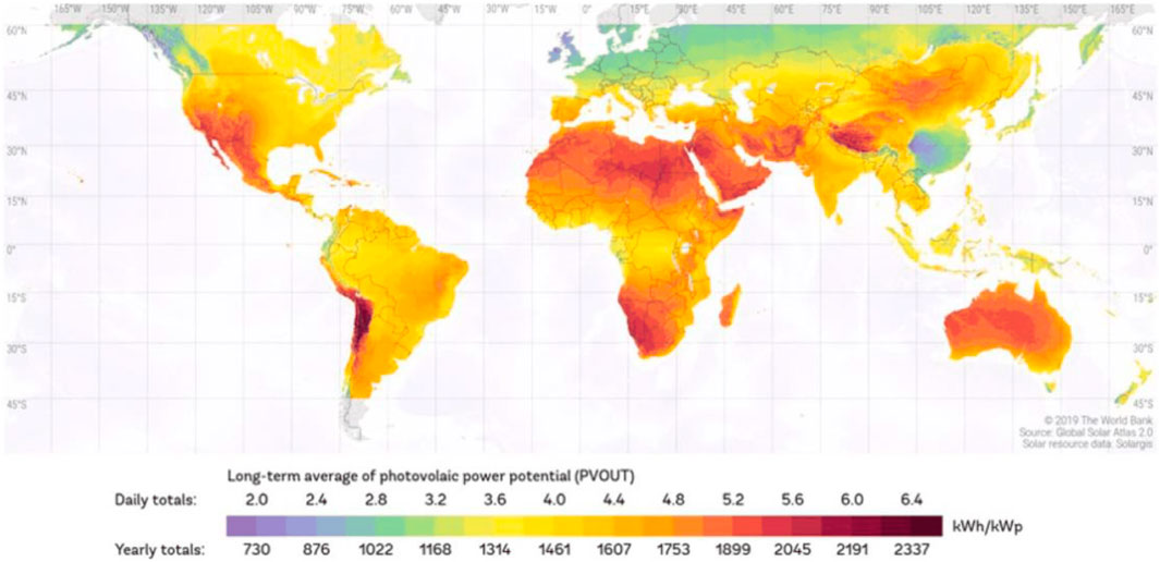
Figure 1. Geographical dispersion of solar resources on a global map Duvenhage (2019).

Three categories of power predicting models are commonly used in the design of electricity power distribution and supply systems: 1) short-term techniques, which provide predicts up to 1 day/week in advance; 2) medium-term models, which extend predictions up to 1 year ahead of time; and 3) long-term models, which have predicted exceeding 1 year Pedregal and Trapero (2010). Ramp events-rapid variations in solar irradiance-are important for very short- and very short-term prediction timeframes. The dependability and quality of PV electricity may decline with sudden and intense fluctuations in solar irradiation. As a result, the best PV power ramp rates can be determined using the results of short-term predictions Lappalainen et al. (2020). Moreover, the enhancement of operational efficiency and market involvement is contingent upon the use of long- and medium-term predicting Husein and Chung (2019). Predictions of day-ahead solar irradiance have proven effective in maximizing annual energy consumption for business operations in microgrids. Consequently, it becomes necessary to modify solar energy projections using a suitable predicting approach and to customize them according to particular applications.

The literature has been overflowing with studies of Saudi Arabia’s wind energy sector in recent years. As Baseer et al. (2017) points out, these studies primarily analyze statistical factors related to various wind farm sites, frequently deriving Weibull distribution parameters for each site. Nevertheless, a significant drawback of this research is their dependence on general evaluations of the available wind speed data for specific locations. As a result, their site productivity results can bespeak that a site is not ideal for a wind project at this time, even though it might be suitable in the future. These studies frequently rely on the presumption that a universal strategy that uses the Weibull distribution works well at every location. This assumption lacks validity and accuracy due to the intrinsic diversity among sites, which could result in over-approximations Ouarda et al. (2015). Interestingly, none of these studies-to the best of our knowledge-have taken into account the addition of wind speed data gathered from other, geographically dispersed places. The lack of such an approach misses the chance to handle these disparate data sets as a single, cohesive package while maintaining the location-based relationships. This comprehensive viewpoint, which is mainly lacking in current research efforts, has the potential to engage in more correct and thorough standard assessments of wind speed productivity at different sites. This paper’s main contribution is to address this specific aspect. The study that is being presented makes use of cutting-edge Artificial Intelligence (AI) approaches that have been widely used in a variety of disciplines. AI is widely used because of its natural benefits in decision-making and model-building Almutairi et al. (2016).

AI techniques have been applied to the research of renewable systems in many studies. The author Almonacid et al. (2010) utilized artificial neural networks to describe solar modules. Other research makes use of data mining methods like fuzzy logic and Support Vector Machines (SVM). Adaptive fuzzy inference systems and Gaussian-kernel SVM are combined in a novel way in Abukhait et al. (2018) to derive fuzzy rules straight from training data for use in testing phases later on. The authors Mansour et al. (2019); Mansour (2018) use of SVM, Artificial Neural Network (ANN), Naïve Bayes, and Decision Tree (DT) is investigated for the analysis of electroencephalography signals in the diagnosis of epilepsy. Furthermore, to detect bad medication reactions, Mansour (2018) use the decision tree technique. A Genetic Algorithm (GA) is then used to optimize the system.

One of the most important steps in attaining a high degree of grid integration of renewable energy is the construction of a comprehensive and centralized Solar and Wind Energy Prediction System (SWEPS). Several essential elements must be included in the improvement of such a method: $(i)$ the capacity to predict loads and predict power output at different time scales (intra-day, day-ahead, and week-ahead); $(ii)$ realistic following and geospatial visualization of renewable generation; and $(iii)$ smooth coordination between grid operators and producers of renewable energy to ensure efficient grid control. With its foundation in accurate power output predictions, the SWEPS is essential in establishing the guaranteed dispatch level for every Renewable Energy Sources (RES) that is accessible. This process is essential for optimal use of energy storage and reducing fluctuations in energy production. Accurate predicting of solar energy requires an extensive apprehension of various components, including the path of the sun, atmospheric conditions, dissipation processes, and the circumstantial properties of the system itself. SWEPS proves effective in finding this complexity and enables the coherent integration of inexhaustible energy into our existing grid system promoting a more authentic and cost-effective energy atmosphere.

The important frameworks embedded into the SWEPS consider $(i)$ a model for Meteorological Numerical Forecasting (MNF), which provides projections of hourly weather data plus solar radiance components Jimenez et al. (2016); $(ii)$ differentiated methodologies for predicting electrical power devoted to different renewable technologies like solar PV and Parabolic Trough Collector (PTC) Zeng et al. (2016); Tang et al. (2015). The determinative information embraced in this methodology involves climate trends, atmospheric compositions, anticipated production from electric power generators as well as traits specific to sustainable energy facilities.

This study lays the foundation for a comprehensive Solar and Wind Energy Predicting System by carefully examining the existing functional frameworks of renewable energy. Using advanced web interface solutions, sustainable energy models, climate predicting modules, and daily updates on solar and weather predictions; SWEPS is designed to effectively monitor the efficiency of various green energy situations. Regular use of this technology will enable grid operators and key players in the Saudi energy sector to provide forward-looking power supply estimates daily. Key objectives include maximizing the current operational locations of RES by facilitating their integration into the unified grid interface while understanding the challenges of connecting or maintaining solar energy systems within the same systematic framework. Additionally, through collaboration with companies such as Elia Grid International, Khalifa University of Science and Technology, and King Abdullah City for Atomic and Renewable Energy (KACARE); Our system advances research by supporting green energy platforms across the region.

In this study, the SWEPS is developed for predicting wind and solar energy. The various data collected across multiple channels is refined and standardized using various pre-processing methods, including deep learning and machine learning algorithms, to predict results. After the initial processing phase, a series of techniques related to Statistical Correlation Analysis (SCA) are used to identify relationships and links between aspects. Least Absolute Shrinkage and Selection Operator (LASSO), Recursive Feature Elimination (RFE), Principal Component Analysis (PCA), Recursive Feature Addition (RFA), and Genetic Algorithm for Feature Selection (GAFS) are some of the techniques used in feature selection. In addition, Cuckoo Search Optimization (CSO), Social Spider Optimization (SSO), Particle Swarm Optimization (PSO), and Neural Network Algorithm (NNA) are GA used to optimize the prediction model to improve its robustness.

The SWEPS represents a significant advancement and contributions in the following.

$•$ For effective solar PV and PTC power predicting, the crucial building blocks are a comprehensive MNF model and specialized predicting methods.

$•$ To ensure high-quality analysis, the data undergoes rigorous refinement and standardization using a diverse toolbox of pre-processing techniques, including machine learning and deep learning algorithms.

$•$ By implementing a combination of feature selection methods such as LASSO, RFE, PCA, RFA, and GAFS, the model’s ability has been improved to identify the most relevant and impactful variables.

$•$ A multi-pronged feature engineering strategy is utilized, combining the Intersection over Union (IoU) technique with various customized methods to enhance model precision and resilience.

$•$ By integrating machine learning models (ANN, Decision Trees, SVM) with deep learning methods (Recurrent Neural Network (RNN), Long-Short Term Memory (LSTM)), a comprehensive and reliable prediction system has been proposed.

$•$ Meta-heuristic optimization techniques (SSO, PSO, CSO, NNA) were employed to fine-tune hyperparameters, achieving near-optimal values for improved convergence and accuracy in models such as SVM, DT, ANN, RNN, and LSTM.

$•$ By applying this holistic approach, asignificant progress have been made in the accuracy and reliability of renewable energy predictions.

Section 1 delves into the latest advancements in Solar and Wind Energy Networks and preprocessing methodologies for Renewable Energy Systems, providing a comprehensive review of cutting-edge works. A summary of the SWEPS is given in Section 3, followed by an examination of the methodological analysis in Section 3.6, methodology development and outcomes in Section 4, and research conclusion and future initiatives in Section 6.

2 Motivation and aims

Predicting solar energy production remains a major hurdle due to the inherent inaccuracies of existing predicting methods, especially when it comes to anomalies in the solar and wind data. Factors such as inconsistencies in energy measurements, inaccurate climate categorization, and variable predicted horizons contribute to unreliable solar intensity predictions. The urgent need for a robust and reliable predicting system that directly addresses these challenges is clear when considering the critical role that solar predictions play in the planning, management, and operation of the global power grid.

In this work, an SWEPS is introduced and presented, an innovative and comprehensive approach to revolutionizing the accuracy and reliability of solar energy prediction. Current predicting techniques often miss the mark due to their limited scope of application. The SWEPS addresses this problem head-on by carefully considering every detail, from the path of the sun to atmospheric fluctuations. This manuscript addresses the complex architecture of SWEPS and shows its dependence on optimization strategies and state-of-the-art preprocessing techniques such as PCA, RFE, LASSO, and RFA-GA. It also highlights how the SWEPS SCA seamlessly integrates with advanced deep learning algorithms. Additionally, it highlights how genetic algorithms such as CSO, SSO, PSO, and NNA are used to refine search criteria and improve model predictability, ultimately paving the way for more accurate and reliable solar energy predictions.

Our dataset’s intricacy and time-series format necessitated a multipronged feature engineering strategy. To make sure the most important features were included, the Intersection over Union (IoU) technique is used in conjunction with a range of customized feature engineering techniques. This strategy made it easier to combine comparable information from several approaches, which improved the overall precision and resilience of our models. In an ensemble framework, also certain machine learning approaches are adopted such as ANN, DTs, and SVM to capitalize on their distinct advantages. Furthermore, deep learning methods are adopted and used that are especially well-suited for time-series forecasting, such as RNN and LSTM networks. By combining these techniques, we were able to develop a thorough prediction system that would function dependably under different circumstances.

Lastly, we highlight the significance of using meta-heuristic optimization approaches to fine-tune our machine learning models’ hyperparameters. To efficiently explore solution spaces, methods like SSO, PSO, CSO, and NNA imitate natural processes. Models like as SVM, DTs, ANN, RNN, and LSTM perform better with this method because it achieves near-optimal hyperparameter values, which guarantee strong convergence and increased accuracy. SWEPS is a vital component for efficient planning and control of the worldwide power grid because it integrates these cutting-edge methodologies to considerably increase the prediction accuracy and dependability of solar and wind energy projections.

3 Proposed design and methodology

This article introduces SWEPS, a novel system for predicting solar and wind energy production. SWEPS addresses data heterogeneity from different sources using a multi-stage process. Algorithm 1 describes the complete process of the proposed methodology. First, it refines and standardizes the data using a powerful combination of deep learning and traditional machine learning algorithms. This pre-processing ensures a clean and consistent basis for subsequent analysis. After the cleaning phase, SWEPS deals with the selection of functions and uses a diverse arsenal of techniques. RFE, PCA, RFA, LASSO, and GAFS. They work together to identify the most impactful features. To illuminate important connections and eliminate redundancies. The optimization of the prediction model takes a central place in the final phase. By using evolutionary algorithms such as GA, SWEPS explores innovative NNA, PSO, SSO, and CSO. This rigorous optimization process improves the robustness of the model and enables it to provide accurate and reliable predictions, ultimately improving grid stability and renewable energy integration.

The SWEPS system, depicted in Figure 2, uses deep learning and machine learning methodology to predict energy usage and production. In the initial step, the dataset from various sources is collected, and remove errors and noise. For normalization, different methodologies are used such as replacing missing values, min-max operation, and standardization on the numerical data. To calculate the correlation, between features, and the selection of optimal features for analysis, we use SCA, RFE, RFA, LASSO, and GAFS to find the optimal correlations. After feature selection, different traditional machine learning algorithms are applied such as SVM, DT, and Neural Networks. Further, we apply the deep learning technique RNN, and LSTM and ensemble these algorithms. To robust our system, optimization algorithms is applied such as NNA, PSO, SSO, and CSO to get the optimal results from the algorithms.

Figure 2

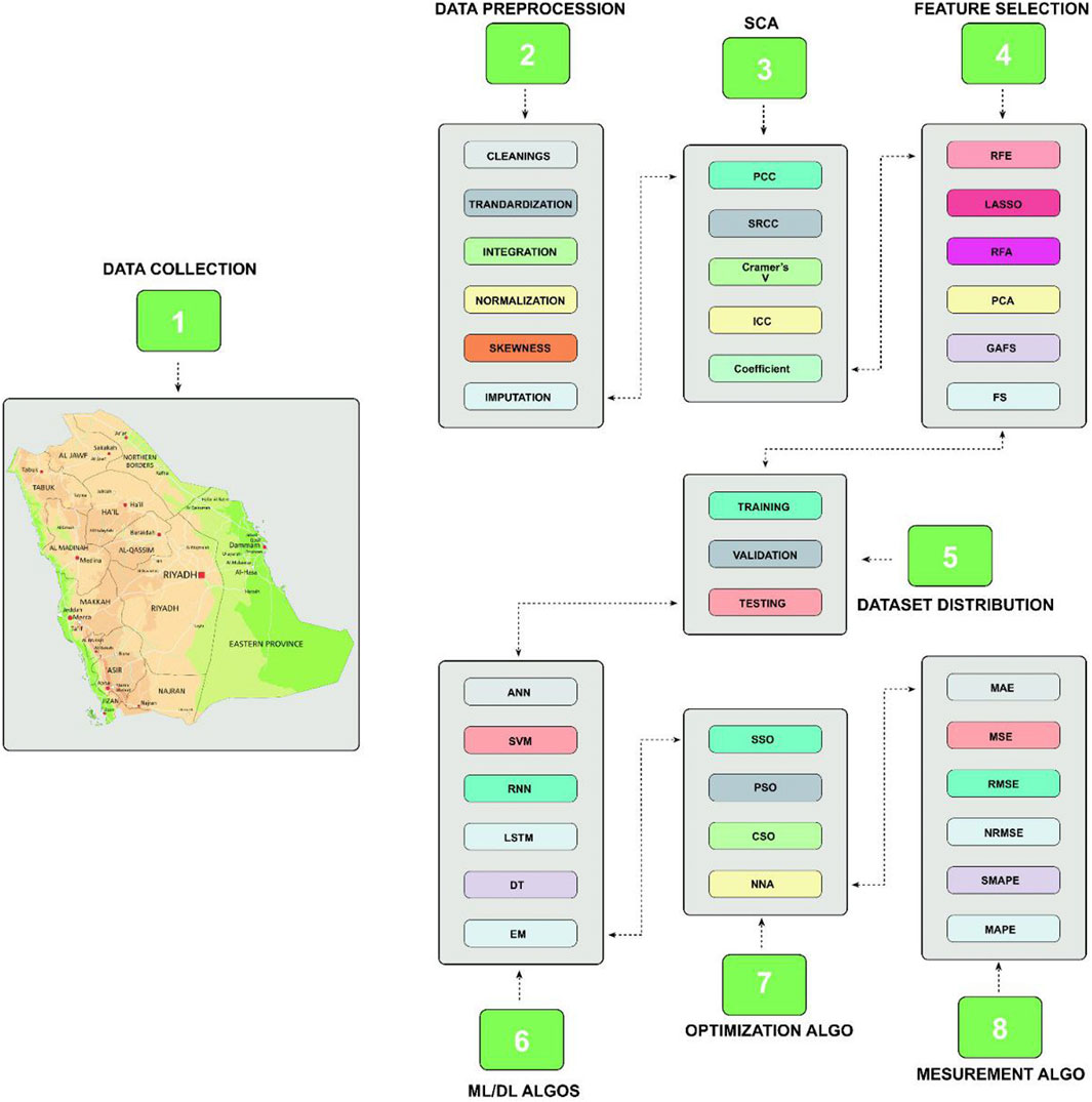
Figure 2. The solar and wind energy prediction system (SWEPS) framework.

3.1 Dataset

We used large datasets of hourly high-resolution solar radiation observations from several years ago, with a combined raw data size of several terabytes. For us to train and validate our deep learning models, such as LSTM and RNN, this massive dataset was essential. It made it possible for us to accurately estimate solar activity and to record temporal dynamics efficiently. The size of the dataset also made it easier to use ensemble methods and meta-heuristic optimization algorithms (PSO, CSO, SSO), which improved our predictions even more. A statistical statement of the data composed at each site is shown in Table 1, which includes indices that provide important information about the location and variability of the data. To help with interpretation, brief descriptions for a few of these statistics are Mean, Standard Error, Median, Mode, Standard Deviation, Sample Variance, Kurtosis, Skewness, and Minimum and Maximum values. The most popular measure of central tendency for a random variable is the mean, which is the average number of data points. Except for the east area, where the recorded mean is 1.9 m/s, the means across the chosen sites range from roughly 3 m/s to 4 m/s. All sites show standard errors below 5%, indicating adequate sample representation. Central tendency measures include median and mode. Standard deviation, variance, kurtosis, and skewness assess data distribution characteristics. Minimum and maximum values denote dataset extremes. Sum and count reveal the total wind speeds and the number of data points. Due to variances in local weather and distances, the data shown in Table 1 show considerable statistical value fluctuations among sites.

Table 1

Table 1. Samples of meteorological data of qassim university.

The information is a component of the KACARE’s Renewable Resource Monitoring and Mapping program. At many locations around the Kingdom of Saudi Arabia, KACARE methodically observed and recorded wind speed data at a height of 3 m. A sample dataset from the different sites is shown in Table 2. The accuracy and degree of confidence in the wind speed estimate are largely dependent on the sample size. Estimates of wind speed are inherently imprecise, and this uncertainty is impacted by the unpredictability of the data as well as sample size; larger samples decrease the uncertainty, while smaller samples increase it. A sample dataset from Qassim University (QU), in Qassin Region in Saudid Arabia as depcited shown in Figure 3, is shown in Table 1, with sample sizes varying from 19,000 to 25,000 data points. To reduce the degree of uncertainty in wind speed estimates, larger samples are purposefully obtained. To tackle outliers, preprocessing involves k-means clustering. It should be noted that the data mining uncertainty is addressed via decision tree methodology, notably Gini impurity and entropy metrics.

Table 2

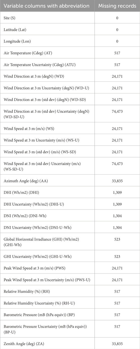
Table 2. Data features.

Figure 3

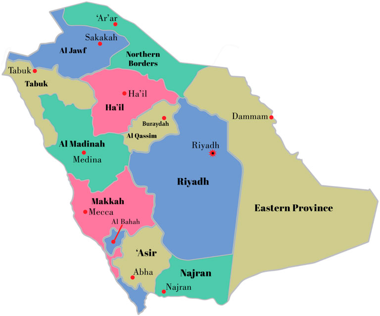
Figure 3. Geographical Saudi Arabia map: Regions.

In Table 2, the number of missing records for each dataset column is displayed in the table. There are large gaps in variables like Wind Direction at 3 m, Wind Speed at 3 m, and related uncertainty. The number of missing values varies depending on the parameter. The information provided makes clear the data gaps that must be taken into account and handled appropriately while analyzing and interpreting the dataset.

3.2 Preprocessing

After a comprehensive examination of the dataset assembled from multiple locations, our data analysis revealed the presence of missing values. To address this issue described in Table 2, we applied certain techniques to numerical and categorical features in our data cleaning strategy. We decided to use imputation for numerical features where data were missing and replace the missing values with the mean of the corresponding features. This helps configure the overall statistical properties of the data set. Instead, we chose to use the mode representing the collection with the highest frequency to fill in missing values for categorical features. This methodology ensures that classification information is presented meaningfully.

After removing missing values, we then standardized all data. When data is normalized, it is transformed so that its mean is zero and its standard deviation is one. Especially when working with algorithms that are sensitive to the scaling of the input variables, this step is essential to ensure that all features contribute equally to the analysis. We have aggregated data from multiple sources into a consistent format to enable in-depth examination across multiple locations. This integration enables meaningful comparisons and analyzes and enables a consistent and consistent presentation. Additionally, we used data normalization techniques to guarantee that numerical values from respective features and locations are immediately comparable. By measuring the mathematical values to a similar range, usually between 0 and 1, normalization removes any potential biases brought about by assorted scales. By taking this step, comparisons are more reliable and the total dataset is interpreted more accurately.

In our careful data analysis, we paid particular attention to dealing with skewness and missing values in columns related to key weather variables. The air temperature $(C\mathrm{deg})$, the wind direction in 3 m $(\mathrm{deg}N)$, the wind speed in 3 m (m/s), the relative humidity (%), and the air pressure (mB (equivalent to hPa)) are just some of those examined Data characteristics. To understand the distribution properties of these features and to detect and correct any asymmetries, an asymmetry assessment is performed. To ensure the completeness and representativeness of the data, missing values in the air temperature and wind direction columns are imputed by replacing the mean and mode, respectively. Similarly, mean, mean, and median-based imputation is used to fill missing values in the wind speed, relative humidity, and barometric pressure columns, respectively. This comprehensive method not only ensures a robust data set but also reduces skewness, providing a basis for deeper analysis and modeling with advisable data quality. The dataset features are Site, Latitude, Longitude, Date, Air Temperature (C$\mathrm{deg}$) – (AT), Air Temperature Uncertainty (C$\mathrm{deg}$) – ATU, Wind Direction at 3 m ($\mathrm{deg}$N) – WD, Wind Direction at 3 m Uncertainty ($\mathrm{deg}$N) – WDU Wind Direction at 3 m (std dev) ($\mathrm{deg}$N) ${\mathrm{W}\mathrm{D}}_{\sigma }$ Wind Direction at 3 m (std dev) Uncertainty ($\mathrm{deg}$N) – ${\mathrm{W}\mathrm{D}\mathrm{U}}_{\sigma }$, Wind Speed at 3 m (m/s) – WS, Wind Speed at 3 m Uncertainty (m/s) – WSU, Wind Speed at 3 m (std dev) (m/s) – ${\mathrm{W}\mathrm{S}}_{\sigma }$, Wind Speed at 3 m (std dev) Uncertainty (m/s) – ${\mathrm{W}\mathrm{S}\mathrm{U}}_{\sigma }$, Azimuth Angle $(\mathrm{deg})$ – AA, DHI (Wh/m2), DHI Uncertainty (Wh/m2) DHIU, DNI (Wh/m2), DNI Uncertainty (Wh/m2) – DNIU, GHI (Wh/m2), GHI Uncertainty (Wh/m2) – GHIU, Peak Wind Speed at 3 m (m/s) – PWS, Peak Wind Speed at 3 m Uncertainty (m/s) – PWSU, Relative Humidity (%) – RH, Relative Humidity Uncertainty (%) – RHU, Barometric Pressure (mB (hPa equiv)) – BP Barometric Pressure Uncertainty (mB (hPa equiv)) – BPU, Zenith Angle $(\mathrm{deg})$ – ZA.

Algorithm 1.Solar and wind energy prediction system (SWEPS).

1: $SWEPS\leftarrow$initialize_SWEPS()

2: $data\leftarrow$collect_data_from_channels ()

3: $refined\_data\leftarrow$preprocess_data ($data$, methods = [missing_values])

4: $processed\_data\leftarrow$initial_processing ($refined\_data$,methods = [normalization, standardization])

5: for alloptimized_results $\ge$threshold do

6:   $selected\_features\leftarrow$feature_selection ($processed\_data$, techniques = [LASSO, RFE,PCA, RFA, GAFS])

7:   $training\_models\leftarrow$learning ($selected\_features$, techniques = [DT, SVM, ANN, RNN, LSTM])

8:   $optimized\_model\leftarrow$optimize_model ($selected\_features$, algorithms = [CSO, SSO, PSO, NNA])

9: end for

10: $output\leftarrow$class_value ($optimized\_model$, algorithms = [MAE, MSE, RMSE, NRMSE, MAPE])

3.3 Statistical correlation analysis

The linear relationship between two continuous variables is measured by the PCC. We may be curious to know the correlation between variables like Air Temperature, Wind Speed at 3m, and Relative Humidity in the context of our dataset. For instance, a positive Pearson Correlation Coefficient (PCC) between temperature and solar radiation would suggest that there is a tendency for solar radiation to rise with temperature. In a similar vein, a negative PCC between temperature and wind speed may indicate an inverse link. The positive association between solar radiation and air temperature follows that solar radiation tends to rise along with air temperature. This is because warmer weather usually means more sunshine and, thus, more solar radiation. A positive PCC value for the association between the variables air temperature and solar radiation that is close to 1 would support the hypothesis that they are positively connected. A negative correlation between temperature and wind speed suggests an adverse relationship. To put it another way, there may be a drop in air temperature and a spike in wind speed. One possible explanation for this connection might be that higher wind speeds provide the illusion of a lower temperature. A negative PCC value would indicate a potential inverse relationship between Wind Speed at 3 m and Air Temperature. When the value of PCC gets closer to −1, the negative link becomes stronger.

In Figure 4, the PCC and Spearman Rank Correlation Coefficient (SRCC) were applied to visualize the relationship between different meteorological features such as air temperature, relative humidity, wind direction, and speed. The values present strong and weak correlations. Positive values indicate a strong correlation and negative values show negative correlations.

Figure 4

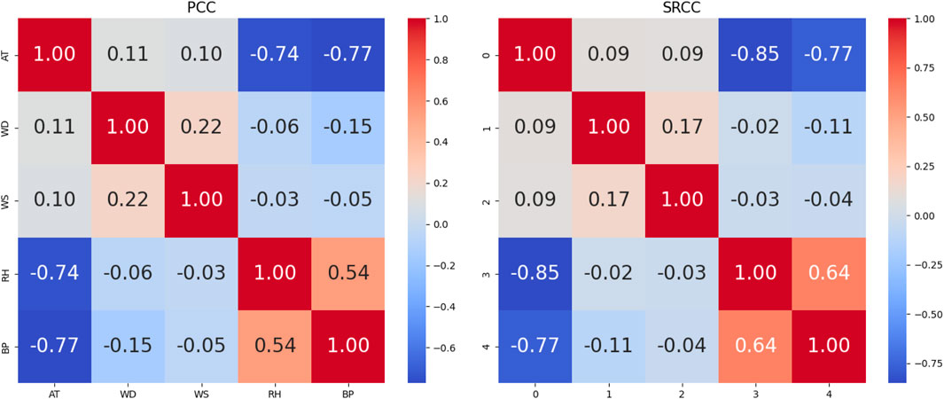
Figure 4. Application of PCC and SRCC to visualize the relationship between different meteorological features.

The monotonic relationship between two variables is evaluated using the SRCC. When working with non-linear relationships, it is quite helpful. Even in cases when the connection between the variables in the dataset is not strictly linear, SRCC can assist in determining whether the variables collectively show a consistent rise or fall in value. Compared to PCC, the rank-based correlation metric SRCC is less susceptible to outliers. The SRCC takes into account the ranks of these values rather than the variables’ actual values. It can withstand extreme values or non-linear relationships because of this. Although the SRCC results may have different numerical values, they should be interpreted similarly to the PCC results. The monotonic relationship between the variables and the correlation direction (positive or negative) should coincide. The SRCC measures the monotonic relationship which should continuously increase and decrease and it does not necessarily have to be linear. It will find the trends between variables which one is falling and rising in proportion to the other. The SRCC values which are near −1 or 1 indicated strong monotonic relationships. When one variable rises, the other tends to rise as well, according to positive SRCC, and when one variable rises, the other tends to fall, according to negative SRCC.

The degree of link between categorical variables is measured using Cramer’s V. We used to analyze the relationship between categorical variables in your dataset, like Wind Direction at 3 m and Wind Speed at 3 m. Between 0 and 1, Cramer’s V denotes the absence of any correlation between the category variables. The Cramer’s V value in the context of wind direction and wind speed should be around zero if there is no regular link between the direction and speed. The Cramer’s V value should be around zero if the wind’s direction and speed are unrelated. A high degree of correlation between categorical variables is indicated by a Cramer’s V value near 1. This would suggest that there is a distinct and well-established link between wind direction and wind speed. The Cramer’s V value should be very near to 1 if wind direction and wind speed are strongly correlated. The consistency or dependability of measurements is evaluated using the Intraclass Correlation Coefficient (ICC). You can use the ICC function in your dataset to determine the degree of consistency in readings for variables such as Air Temperature and Wind Speed at 3 m across several sites. In $2\times 2$ contingency tables, the association is measured by the $\varphi$ Coefficient. You might utilize the $\varphi$ Coefficient in your dataset to determine the relationship between categorical variables such as Peak Wind Speed at 3m and Wind Direction at 3m. Particularly in the uncertainty metrics across all records, Table 2 has considerable missing data in several of its columns. To maintain the accuracy and dependability of the dataset, it has been adopted to exclude some columns from the study.

3.4 Feature engineering

The main objective of this research is to use data from an Solar and Wind Energy (SWE) located at Qassim University in Saudi Arabia to anticipate SWE power generation. Three different kinds of factors that are pertinent to the study location are used to train different models to get the most accurate SWE power production prediction. The literature has shown that temporal parameters, meteorological circumstances, and historical SWE power-generating data have a significant impact on SWE output. The input variables used in this study are listed in Table 2. As an example, the air temperature ($\mathrm{deg}$C) is represented by variable (d$4_m$), where m is the temperature value for each hour, yielding 24 values per day. The dataset (D) is then divided into three subsets, namely the validation, the test dataset, and the training dataset. In this study, 15% and 10% of the data is set aside for validation and testing, respectively and the remaining 75% is used for training. To optimize hyperparameters for conventional machine learning algorithms and set up the neural network architecture the K-fold validation technique is utilized.

The target column is removed from the dataset before it is imported into a unique format to create the feature matrix, represented by the letter X. After that, PCA is performed to X, converting the data into a space with fewer dimensions. To help with the decision of how many components to keep, it includes a plot depicted in Figures 5, 6, that shows the cumulative explained variance ratio against the number of principal components. To further visualize the data in the condensed space, optional 2D and 3D scatter plots are generated. A deeper comprehension of the dataset’s underlying structure is made possible by these visualizations, which provide insights into the patterns and relationships found within it.

Figure 5

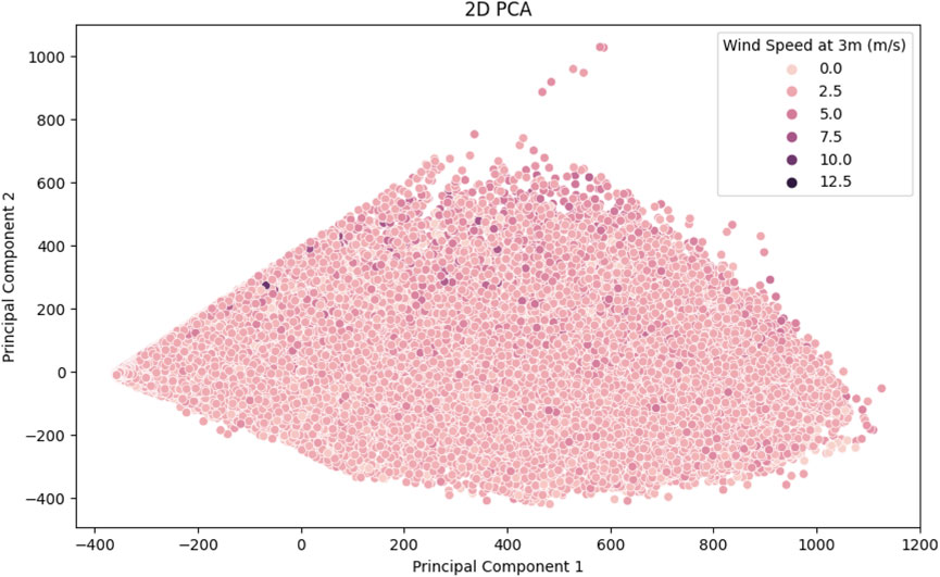
Figure 5. PCA 2D.

Figure 6

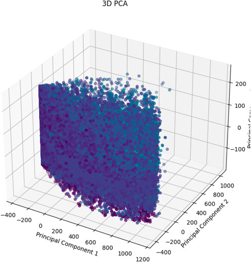
Figure 6. PCA 3D.

In Figures 5, 6, the additive elaborate variance ratios for all important elements obtained from PCA are presented in this figure. The number of primary components is plotted on the x-axis, while the cumulative explained variance ratio is plotted on the y-axis. The plot aids in figuring out the ideal number of primary components required to preserve a sizable portion of the original dataset’s content.

The determined computer and a planned amount of selectable features are used to format RFE. After fitting the RFE model to the data, a horizontal bar chart is used to illustrate the ranking of features and help determine which features are most important in predicting the” Diffuse Horizontal Irradiance (DHI) $(Wh/m^2)$”. This method preserves the most relevant features, simplifies the dataset, improves model interpretation, and can even increase prediction performance. This is useful for feature selection, as Figure 7 shows.

Figure 7

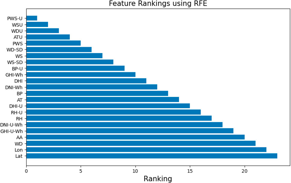
Figure 7. Feature rankings via RFE for predicting solar and wind energy.

Feature Rankings via RFE for Predicting Solar and Wind Energy. The significance of each attribute in predicting DHI with the Random Forest Regressor as the estimator is displayed as a horizontal bar plot. Features are rated according to how well they predict the model performs, which helps identify the important factors affecting solar radiation. RFE is a useful approach for feature selection since it keeps the most important variables in the model, improving interpretability and possibly optimizing prediction accuracy.

Initially, the selected and objective feature is removed from the source dataset and the remaining features are there in the dataset for analyzing and predicting the objective features. Using $\alpha$ variable of 1.0 is used in the LASSO regression model to regularize the degree of parameters. The dataset fits and is trained on the model and develops the coefficients for each attribute presented in Section 3.4. Two visualizations are created: a two-dimensional plot in Section 3.4 showing the LASSO coefficients versus the feature indices. With these interactive visualizations, you can readily explore how each factor shapes the target variable, ultimately leading to the identification of crucial features for further research or model construction. The “alpha” parameter serves as a customizable lever, empowering you to fine-tune the feature selection method based on the specific needs of your data and modeling ambitions.

The complicated dynamics and time-series character of our data in our study made it difficult for us to use a single strategy for feature engineering. A variety of feature engineering strategies is used that were adapted for our particular dataset to solve this. Every unique method extracted pertinent characteristics that are essential to our prediction model. The Intersection over Union (IoU)approach is used to make sure the most relevant and appropriate characteristics were included. By locating and combining similar features from different engineering methodologies, IoU made it easier to integrate features. By using this strategy, we made sure that our prediction system had access to a wide range of information that improved our models’ overall accuracy and resilience and increased our capacity to accurately forecast the dynamics of solar and wind energy.

As in Section 3.4 the effect of each feature on the target variable “DHI (Wh/m2)” is illustrated in this bar chart, which shows the coefficients derived from the LASSO regression model (Figures 8, 9). The magnitude of the coefficients is represented by the x-axis, with positive and negative values representing the direction and strength of the connection, respectively. Features with non-zero coefficients significantly increase the predictive ability of the model and help identify important factors in predicting solar radiation.

Figure 8

Figure 8. 2D Features Coefficients using LASSO Coefficients for Features Selection.

Figure 9

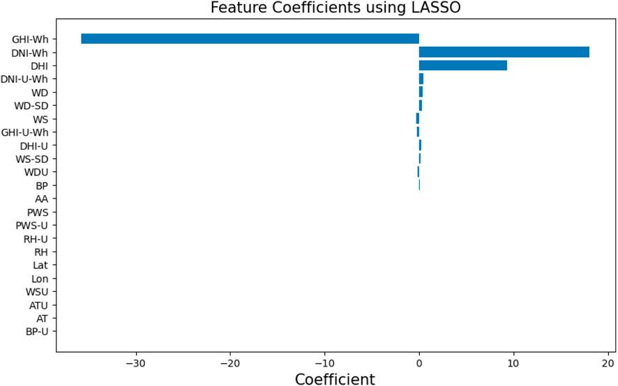
Figure 9. Features Coefficients using LASSO regression model.

3.5 Machine learning algorithms

Gaining knowledge about these linear correlations will help you better understand how solar irradiance behaves and the elements that influence it. For instance, clear skies, lower relative humidity, and higher air temperatures are often linked to high solar irradiance (GHI and DNI), but overcast days with greater humidity might result in higher diffuse irradiance DHI. The zenith angle, wind direction and speed, and barometric pressure all have a major impact on how weather patterns shape solar energy availability. Improved models for forecasting solar irradiance and optimizing renewable energy systems may be created by examining these correlations.

The key to determining how changes in one variable might affect another is to comprehend the linear relationships between the columns depicted in Figure 10, ‘Air Temperature (C$°$)’, ‘Wind Direction at 3 m (N$°$)’, ‘Wind Speed at 3 m (m/s)’,’ Direct Normal Irradiance (DNI) (Wh/${\mathrm{m}}^2$)’, ‘GHI (Wh/${\mathrm{m}}^2$)’, ‘DHI (Wh/${\mathrm{m}}^2$)’, ‘Relative Humidity (%)’, ‘Barometric Pressure (mB (hPa equiv))’, and ‘Zenith Angle $(◦)$’. Since clear, sunny days tend to be warmer, higher air temperatures are typically correlated with enhanced GHI. Similarly, because of the brighter sky, DNI and DHI may increase with temperature. While wind direction may affect humidity levels depending on the source of the air masses, the link between wind direction and speed might indicate regional weather trends. The dispersion of clouds and the mixing of air masses caused by wind speed can both influence solar irradiance levels and humidity. Given that GHI is made up of both DNI and DHI, a strong linear connection between the two is anticipated. Due to greater solar radiation, higher DNI values are frequently correlated with higher temperatures. DNI is also influenced by the sun’s zenith angle, with lower zenith angles generally translating into higher DNI values.

Figure 10

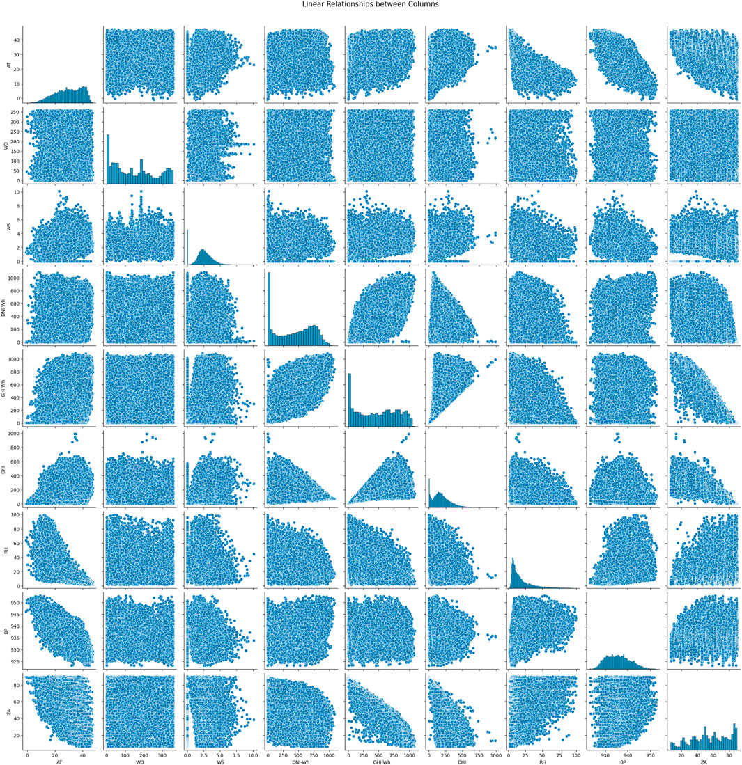
Figure 10. Solar irradiance correlates with meteorological variables like temperature, wind, humidity, and atmospheric pressure. Higher irradiance GHI aligns with increased temperatures and clearer skies, boosting both diffuse DHI and direct DNI irradiance. Wind affects humidity and cloud dispersion, influencing irradiance. Solar angle impacts intensity, while humidity scatters light, enhancing DHI. Barometric pressure links to humidity: low pressure increases cloudiness, while high pressure clears skies. These relationships refine solar energy prediction models.

The zenith angle also affects GHI because irradiance is often increased at lower angles. Relative humidity and DHI have a noteworthy relationship because high humidity can scatter sunlight, boosting DHI even in the presence of cloud cover, which lowers GHI and DNI. Weather systems influenced by barometric pressure have an impact on humidity levels; high-pressure systems are often linked to clear skies and reduced humidity, while low-pressure systems are linked to higher humidity and cloudiness. Additionally, through cloud cover and irradiance levels, there is an indirect link between relative humidity and the zenith angle. Since low-pressure systems can be warmer, high-pressure systems are often associated with cooler temperatures because of radiative cooling and clear sky. A surface’s exposure to solar radiation is directly influenced by its zenith angle; a lower zenith angle (the sun is higher in the sky) means a higher irradiance. These linear correlations shed important light on how solar irradiance behaves and what influences it. For example, DHI might be higher on overcast days with increased humidity, whereas high solar irradiance (GHI and DNI) is often linked with clear sky, reduced relative humidity, and higher air temperatures. The zenith angle, wind direction and speed, and barometric pressure all have a major impact on how weather patterns shape solar energy availability. Improved models for forecasting solar irradiance and optimizing renewable energy systems may be created by examining these correlations.

A decision tree effectively divides the input space of a data set into different, non-overlapping parts and gives each region a different name. The decision tree starts from the root node and reaches the last leaf nodes Perez et al. (2013), with multiple branches connecting these locations. The algorithm makes decisions by iteratively dividing the data into multiple parts and then dividing each region into even smaller partitions. The elimination operations are recursively executed until we reach the last node. The contamination metric is the default-based partition. In our study, the main measurement metric is entropy and it finds the homogeneity between separated nodes. The finding of entropy is a recursive step-wise procedure in decision tree algorithm and it is controlled by Gini Index and entropy as the primary scale of impurity. The depicted Equations 1, 2 is a group of mathematical equations that depicts the requirements of separating nodes from the root and constructing a decision tree. To find the measures of impurity via entropy (H) and the Gini Index (GI), the depicted Equations 1, 2 completely rely on it. The Gini index for a given tree node can be found as follows:

$GI=1-{\displaystyle \sum _{i=1}^C}{p}_i^2(1)$

where $p_i$ is the probability that class $i$ will occur in the node, and $C$ is the number of classes. $H$ stands for entropy, which is computed as follows:

$H=-{\displaystyle \sum _{i=1}^C}{p}_i\cdot {\log }_2\left(p_i\right)(2)$

where ${\mathrm{p}}_i$ presents the likelihood that class i will present in the node and C depicts the number of classes. One of the powerful predictive algorithms is a decision tree that indicates the relationship in the provided dataset, such as “WHI(Wh/m2)” is the root/based node, it suggests the features are important when finding the outcomes of the decision tree. The decision tree probably used the main feature of “GHI” to split the dataset into different branches. The outcomes of each subtree heavily rely on the particular features that are used in that subtree and these outcomes are presented by leaf nodes and expecting the results. Another main feature of solar radiation is GHI and its location may be a base node indicating that it has a significant influence on the prediction of other parameters. Analyzing the decision tree’s composition is crucial since it presents the hierarchy of features according to how they are predictive. Decision trees also offer interpretability, which enables involved parties to embrace the parameters affecting the systems’s outcomes. Insights into the dynamics of solar radiation and climatic parameters affecting the dataset can be gained if particular GHI thresholds or circumstances are located in the decision tree.

For regression and classification problems, one of the widely applied algorithms is SVM. In our system, we apply to predict the solar and wind energy, and to robust our proposed system. The main agenda of SVM is to search for the optimal hyperplane in a high-dimensional space to partition data points. For binary classification problems, Equation 3 for predicting solar and wind parameters is written as follows:

$Y=\text{sign}\left({\displaystyle \sum _{i=1}^n}{\alpha }_i{y}_{i}K\left(x_i,x\right)+b\right)(3)$

Here, $Y$ is the predicted output. ${\alpha }_i$ are the Lagrange multipliers. $y_i$ is the target output for the $i$-th data point. $x_i$ represents the feature vector for the $i$-th data point. $x$ is the input feature vector for prediction. $K(x_i,x)$ is the kernel function, mapping data points to a higher-dimensional space. SVM attempts to penalize misclassifications while maximizing the difference between classes. Regression or multiclass situations may require changes to the SVM equation. SVM predicts solar or wind power for a power graph based on provided factors such as air temperature, wind speed, latitude, longitude, etc. SVM efficiently process high-dimensional feature spaces for accurate predictions and are robust to missing data. The choice of kernel function, such as a polynomial or radial basis function (RBF), is noteworthy and depends on the properties of the data. The available datasets are used to learn the SVM model and the generated hyperplane is used to predict new data points.

Even in the absence of data, ANN, computer models designed on the structure of the human brain, can successfully predict solar and wind hidden patterns. The general ANN equation depicted in Equation 4 $\mathit{\text{X}}$ and the target output as $\mathit{\text{Y}}$ looks like this:

$Y=f\left(W_{\text{input\_hidden}}\cdot X+b_{\text{hidden}}\right)(4)$

Here, $W_{\text{input\_hidden}}$ is the weight matrix. $b_{\text{hidden}}$ is the bias vector. $f$ is the activation function. To predict solar or wind parameters, this equation is adjusted using data such as latitude and longitude, date, air temperature, and wind speed. ANN deals with missing data sets by extracting insights from available data to make accurate predictions. A well-generalizing model that can make accurate predictions under a range of circumstances is the aim.

One kind of artificial neural network that works particularly well for training sequential or time-series data is the RNN, which is capable of handling time-series data, which includes important temporal information, in contrast to Simple Neural Networks Hüsken and Stagge (2003). To represent input at various time intervals, RNN deconstructs sequences into their parts and keeps a state Hochreiter and Schmidhuber (1997). The RNN structure, comprises inputs, hidden neurons, and an activation function. Equation 5 defines the preceding hidden layer (${\mathrm{h}}_t$):

$h_t=\tanh \left(U\cdot x_t+W\cdot h_{t-1}\right)(5)$

In this case, the input is denoted by ${\mathrm{x}}_t$, the hidden neuron is represented by ${\mathrm{h}}_t$, the weight of the hidden layer at time t is represented by U, and the transition weights of the hidden layer are denoted by W. The $tanh$ function functions as a Neural Network Memory to store information from previous iterations by combining current and past inputs to build a new hidden state.

An improved version of the RNN, the LSTM network addresses problems with long-term data dependencies and time-series predicting, which are frequently hampered by gradient explosion and vanishing gradient problems. The LSTM architecture in Figure 6 comprises inputs, memory cells, outputs, and forget gates that act collectively to control information flow. The forget gate splits what should be retained and discarded. The output gate ascertains the subsequent hidden state, whereas the input gate updates the cells. By producing values between 0 and 1, sigmoid functions trigger the gates, allowing information to get through only in certain cases. Equation 6 describes this mathematical structure in detail:

$f_t=\sigma \left(w_f\cdot h_{t-1}+w_f\cdot x_t+b_f\right)(6)$

The sigmoid activation function is represented by $\sigma$ in this case, the weight matrix is ${\mathrm{w}}_f$, the previous state is ${\mathrm{h}}_{t-1}$, the input vector’s memory cell at time tt is ${\mathrm{x}}_t$, and the bias vector is indicated by ${\mathrm{b}}_f$.

$C_t^{\sim }=\tanh \left(w_c\cdot h_{t-1}+w_c\cdot x_t+b_c\right)(7)$

$i_t=\sigma \left(w_i\cdot h_{t-1}+w_i\cdot x_t+b_i\right)(8)$

$C_t=i_t\cdot C_t^{\sim }+f_t\cdot C_{t-1}(9)$

$O_t=\sigma \left(w_o\cdot h_{t-1}+w_o\cdot x_t+b_o\right)(10)$

$h_t=\tanh \left(C_t\right)\cdot O_t(11)$

Using the sigmoid activation to identify values to compose and the tanh activation function to update the gate with new cell values, the input gate ${\mathrm{i}}_t$ decides the data stored in the new cell state ${\mathrm{C}}_t^{\sim }$. Equations 7–11 updates the most recent cell state ${\mathrm{C}}_t$ by combining the candidate cell state ${\mathrm{C}}_t^{\sim }$ and the previous cell state ${\mathrm{C}}_{t-1}$. To compute the final output ${\mathrm{h}}_t$, the output gate ${\mathrm{O}}_t$ regulates cell output by combining it with a cell state activated through the tanh function.

A feature ensembling algorithm that concatenates features from DT, SVM, ANN, and RNN with features from other deep learning models. By combining the advantages of several models, this strategy seeks to produce a more reliable and accurate prediction system for solar and wind parameters. The specific features that are highlighted-DHI, DHI Uncertainty, DNI, DNI Uncertainty, GHI, and GHI Uncertainty-are the main emphasis of the assembling process. RNN and LSTM are good at identifying temporal and sequential patterns in time-series data, which makes them appropriate for features such as air temperature, wind direction, and wind speed (Figures 11, 12). Ensembling is the process of combining the pertinent features that are taken out of RNN and LSTM models, probably including some that have to do with the intrinsically temporal nature of wind and solar data. Non-linear correlations and interactions between features can be handled via decision trees. SVM performs effectively in high-dimensional areas and has good data handling capabilities. An ANN is a flexible model that can extract intricate patterns from data. These models probably make use of latitude, longitude, and atmospheric parameters (such as pressure, temperature, and humidity). Concatenation of relevant features from the standard models (DT, SVM, ANN) and deep learning models (RNN, LSTM) is performed. With this combination of features, deep learning, and conventional machine learning techniques are used to capture an extensive set of data. Combining the predictions of separate models-possibly using methods like weighted voting, stacking, or averaging-is the ensembling process. Important solar irradiance metrics that indicate various portions of sunlight that reach the Earth’s surface are DHI, DNI, and GHI. The uncertainty values offer valuable information regarding the dependability of the relevant measurements of irradiance. Incorporating these elements guarantees that the assembling procedure takes into account the minute nuances of solar radiation, which is necessary for precise solar and wind predicting. To provide a more authentic and precise solar and wind predicting system, the assembly process involves balancing the different capabilities of traditional deep learning and machine learning models. The prediction model is generally more reliable because taking individual characteristics into account ensures that the peculiarities of solar radiation intensity are carefully taken into account.

Figure 11

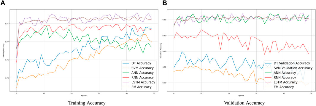
Figure 11. Comparative Analysis of training and validation accuracy of various learning models: Assessing the performance of traditional machine learning algorithms (DT, SVM, ANN), deep learning algorithms (RNN, LSTM), and EM models. Results showcase model accuracy without the application of optimization algorithms.

Figure 12

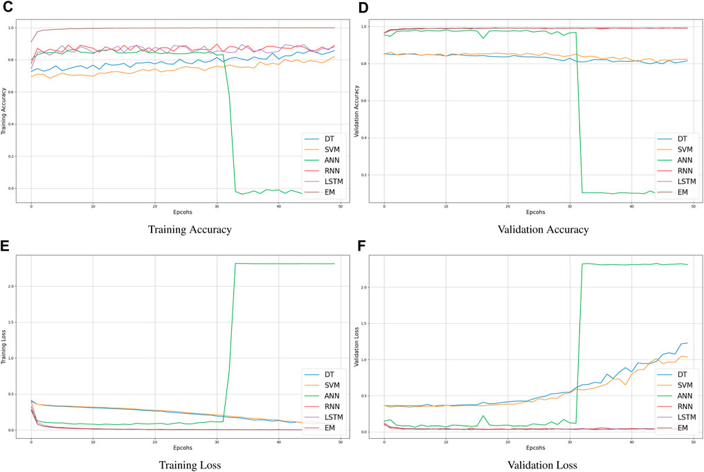
Figure 12. Training and Validation Accuracy of learning models: We use different traditional machine learning algorithms (DT, SVM, ANN) and deep learning algorithms (RNN, LSTM) and EM models. The results are obtained without optimization algorithms.

We used specific machine learning methods such as Decision Trees, Support Vector Machines (SVM), and Artificial Neural Networks (ANN) in addition to an ensemble approach to combine their advantages. This ensemble approach uses the unique strengths of each model to capture various aspects of the dataset, hence increasing the prediction potential. To be more precise, SVM is good at establishing intricate decision boundaries in high-dimensional spaces, whereas Decision Trees are good at exposing nonlinear connections and interactions among features. By extracting deeper insights from data, ANN enhances these models with its adaptability in learning complex patterns. Our goal in assembling these conventional machine learning algorithms was to obtain a thorough comprehension of solar and wind energy forecasts.

Furthermore, we expanded this strategy to incorporate deep learning techniques including Long Short-Term Memory (LSTM) networks and RNN. Because RNNs are designed to handle sequential data, they are appropriate for time-series forecasting, which is a necessary component of solar and wind energy prediction. Long short-term memory networks (LSTMs), which are well-known for managing long-term dependencies, significantly improve the model’s capacity to accurately represent temporal dynamics. We combined the complimentary characteristics of these deep learning architectures with the conventional models to create a single prediction system. Our prediction models for solar and wind energy are more reliable because to this combination of deep learning and machine learning techniques, which guarantees stable performance across a range of circumstances.

Accurate tuning of hyperparameters is crucial to the performance of machine learning models, including DT, SVM, and LSTM. For SVM, the regularization value C is normally between 0.1 and 1000 to account for training and testing errors. The kernel factor $\gamma$, which sets the decision boundary, and choosing an appropriate kernel impact type are other crucial elements to consider. Suggested ranges, on the other hand, for DT features such as maximum depth, minimum sampling distribution, and minimum sample sizes are normally from 1 to 32, from 2 to 20, and from 1 to 10. When you delve into the field of LSTM networks, variables such as batch size, number of epochs, learning rate, dropout rate, and number of LSTM units become critical. The fraction of input units lost during training, or the dropout rate, typically ranges between 0.2 and 0.5, while the learning rate typically ranges between 0.1 and 0.0001.

3.6 Optimization methodology

Machine learning models like SVM, DT, ANN, RNN, and LSTM perform better when meta-heuristic optimization algorithms like SSO, PSO, CSO, and NNA are used. By rapidly exploring and exploiting solution spaces, these optimization algorithms are made to resemble the behaviors of natural systems, which enables them to identify near-optimal solutions in high-dimensional, difficult situations.

SSO uses a traditional hunting style Social Spdier’s to train the model. During learning, it animates the sub-spider to analyze together and boost the performance of a model using feature engineering. Through more efficient solution space exploration, SSO aids in the discovery of ideal hyperparameters for SVM, DT, ANN, RNN, and LSTM. The SSO equation is depicted in Equation 12 for spider (i) exploration:

$x_i\left(t+1\right)=x_i\left(t\right)+\alpha \cdot \text{rand}\left(\right)\cdot \text{dist}\left(x_i,x_{\text{best}}\right)(12)$

where $x_i(t)$ is the location of spider $i$ at time $t$, $\alpha$ is a constant, rand () generates a random number between 0 and 1, and dist (${\mathrm{x}}_i$, ${\mathrm{x}}_{\text{best}}$) is the Euclidean distance between the location of spider $i$ and the best locations in the population.

In searching for the best possible outcomes, the PSO depicted in Equations 13–15 simulates how a particle swarm might work. It applies to adjusting the hyperparameter weights in getting optimal results for RNN, DT, SVM, ANN, and LSTM models. It provides the ability to balance the exploration and production for optimal convergence and learning performance. For updating the position of the particle i and velocity are given by.

$v_i\left(t+1\right)=w\cdot v_i\left(t\right)+c_1\cdot {\text{rand}}_1\left(\right)\cdot \left(p_{\text{best}}-x_i\left(t\right)\right)(13)$

$\alpha =c_2\cdot {\text{rand}}_2\left(\right)\cdot \left(g_{\text{best}}-x_i\left(t\right)\right)(14)$

$x_i\left(t+1\right)=x_i\left(t\right)+v_i\left(t+1\right)+\alpha (15)$

Where $w$ is the inertial mass, $c_1$ and $c_2$ are the acceleration coefficients, ${\text{rand}}_1()$ and ${\text{rand}}_2()$ generates random numbers, $p_{\text{best}}$ is the best position of the particle and $g_{\text{best}}$ is the best position among all particles.

The reproductive parasitism of some cuckoo species was used as a model for the CSO presented in Equation 16. It is used to replace worse solutions with better solutions to optimize the model parameters. CSO helps you efficiently navigate the search space, avoid local optima, and build more accurate models in SVM, DT, ANN, RNN, and LSTM. The equation for updating the position $i$ of the cuckoo is given by:

$x_i\left(t+1\right)=x_i\left(t\right)+\alpha \cdot L\cdot \text{Levy}\left(\right)(16)$

where $\alpha$ is a step size, $L$ is the scaling factor, and Levy () generates a Levy flight.

An NNA is a meta-heuristic inspired by the composition and functioning of the human brain. This works great for hyperparameters and neural network design optimization. When NNA is used with SVM, DT, ANN, RNN, and LSTM, it helps to find the best network configurations and improve model accuracy. By integrating these meta-heuristic optimization algorithms into the training and optimization processes of machine learning models, the benefits of advanced exploration of the solution space enable the identification of optimal hyperparameters and model configurations. This results in better performance across a wide range of tasks, making models more adaptable and efficient, and capable of producing reliable results in real-world applications.

Meta-heuristic optimization techniques require careful tuning of hyper-parameters to produce meaningful results. The scaling factor $(\alpha )$, the impact factor $(\beta )$, and the decay factor $(\perp )$ are important variables in SSO. Actual performance is generally achieved by setting $\alpha$ between 0.1 and 2, $\beta$ between 0.1 and 2, and $\perp$ between 0.1 and 2. Likewise, it is important to change the inertial weight (w), the cognitive acceleration factor $(c_1)$, and the social acceleration factor $(c_2)$ when PSO. For w the recommended ranges are generally between 0.1 and 1.4 and for $c_1$ and $c_2$ between 1 and 2. The step size $(\alpha )$ and the scaling factor (L) are used in CSO. Recommended values for $\alpha$ and L are in the range of 0.1–1 and 1 to 3, respectively. In addition, the learning rate of the NNA that calculates the optimization step size must be between 0–1 and 0.001. The architecture of the neural network ascertained by the number of neurons and hidden layers plays an important role in the optimization process. These algorithms can navigate solution spaces more efficiently by efficiently adjusting the proposed domains, thereby providing reliable and better results in a variety of applications. The significance of using meta-heuristic optimization techniques in adjusting machine learning models’ hyper-parameters is emphasized in this section. To successfully search and exploit solution spaces, techniques like SSO, PSO, CSO, and NNA imitate natural processes. Finding nearly optimal hyperparameter values as a result improves the functionality of models such as SVM, DT, ANN, RNN, and LSTM. These algorithms provide strong convergence and increased model accuracy by striking a balance between exploration and exploitation, which makes them essential tools for creating high-performing predictive models.

3.7 Measurement metrics

When evaluating the performance of machine learning models such as SVM, DT, and LSTM networks, the measurement parameters listed below in Equations 17–22 are essential.

$\mathrm{M}\mathrm{A}\mathrm{E}=\frac{1}{n}{\displaystyle \sum _{i=1}^n}|y_i-{\widehat{y}}_i|(17)$

$\mathrm{M}\mathrm{S}\mathrm{E}=\frac{1}{n}{\displaystyle \sum _{i=1}^n}{\left(y_i-{\widehat{y}}_i\right)}^2(18)$

$\mathrm{R}\mathrm{M}\mathrm{S}\mathrm{E}=\sqrt{\mathrm{M}\mathrm{S}\mathrm{E}}(19)$

$\mathrm{N}\mathrm{R}\mathrm{M}\mathrm{S}\mathrm{E}=\frac{\mathrm{R}\mathrm{M}\mathrm{S}\mathrm{E}}{\text{max}\left(y\right)-\text{min}\left(y\right)}(20)$

$\mathrm{S}\mathrm{M}\mathrm{A}\mathrm{P}\mathrm{E}=\frac{1}{n}{\displaystyle \sum _{i=1}^n}\frac{|y_i|+|{\widehat{y}}_i|}{2}\frac{|y_i-{\widehat{y}}_i|}{|y_i|}(21)$

$\mathrm{M}\mathrm{A}\mathrm{P}\mathrm{E}=\frac{100}{n}{\displaystyle \sum _{i=1}^n}\frac{|y_i-{\widehat{y}}_i|}{|y_i|}(22)$

The Mean Absolute Error (MAE) between the actual values (${\mathrm{y}}_i$) and the predicted values $({\widehat{y}}_i)$ is shown. Provides an easy way to measure model accuracy. The average squared difference between the expected and actual values is computed by Mean Square Error (MSE). Squaring increases the emphasis on greater errors, which makes outliers more noticeable. Because it is expressed in the same units as the target variable, Root Mean Square Error (RMSE) - the square root of MSE - is easier to understand. Compared to MAE, it penalizes bigger errors more severely. A normalized measure of error is obtained by scaling RMSE by the target variable’s range, a process known as Normalized Root Mean Square Error (NRMSE). By taking into account the average of their magnitudes, Symmetric Mean Absolute Percentage Error (SMAPE) determines the percentage difference between the projected and actual values. It works well with datasets that contain zero values and is symmetric. Concerning the actual values, Mean Absolute Percentage Error (MAPE) calculates the percentage difference between the predicted and actual values. It gives the inaccuracy as a percentage and is frequently used in predicting.

4 Experimental results

The number of neurons in hidden layers is an important step in the context of ${\mathrm{T}\mathrm{e}\mathrm{r}\mathrm{m}}_A$ and ${\mathrm{T}\mathrm{e}\mathrm{r}\mathrm{m}}_B$, especially when using LSTM networks. To achieve this, the optimization method uses SSO, PSO, CSO, and NNA. Finding the best configuration for an LSTM architecture is facilitated by metaheuristic methods. However, ${\mathrm{T}\mathrm{e}\mathrm{r}\mathrm{m}}_C$, which uses an RNN, is based on a simpler structure. This system comprises an input layer, a hidden layer, and an output layer. Table 3 presents that the number of neurons in the hidden layer represents the number of input features. For example, an instance with single feature is allotted one node, while an instance with multiple features is assigned to different multiple nodes. To maintain dataset consistency, LSTM models use the same input data as RNN models. Table 4 provides a detailed summary of the configuration of the best LSTM models after applying various optimization strategies. SVM technique uses the default settings, with C set to unity for linear and radial basis functions. The reciprocal of the number of features gives the parameter $(\gamma )$. Then, appropriate network parameters and configurations are used in SVM and LSTM models to accurately predict PV power generation. Several evaluation variables are used to evaluate the predictive performance of the models; The results are shown in Table 5. This comprehensive study provides a comprehensive understanding of the performance of SVM, RNN, and LSTM models in the context of PV power generation predicting, as well as information on the degree of agreement between predicted and measured data.

Table 3

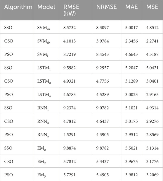
Table 3. Comparison of predicting Models Using SVM, LSTM, RNN, and EM with Meta-Heuristic Algorithms (SSO, CSO, PSO with single feature (DHI $(Wh/m^2)$).

Table 4

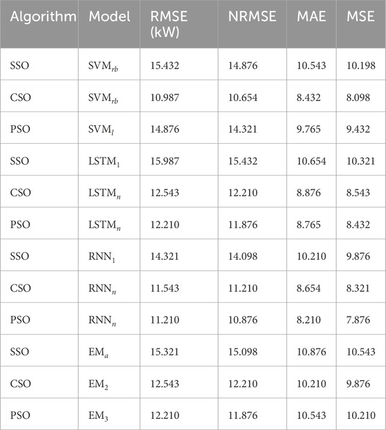
Table 4. Assessment and Comparison of the SVM, LSTM, RNN, and EM as predicting models with unique features (Wind Direction at 3m, GHI $(Wh/m^2)$, and DNI). The optimization are achieved through meta-heuristic algorithms (SSO, CSO, PSO).

Table 5

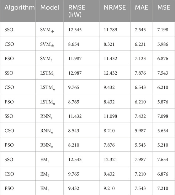
Table 5. Achievement analysis of SVM, LSTM, RNN, and EM as predicting models with distinct features (Wind Direction at 3 m (N), DHI $(Wh/m^2)$, and DNI $(Wh/m^2)$). The results are optimized through meta-heuristic algorithms (SSO, CSO, PSO).

In this section, we address the analysis and debate about the effectiveness of current solar irradiance prediction models based on deep learning. Currently, the most popular method for predicting solar radiation intensity is the LSTM. Its popularity comes from being a type of RNN that gives the network more storage capacity in addition to preserving data for later use. Because it can reveal long-term correlations within time series data and speed up the convergence of non-linear predictions, this model is often used for predicting solar irradiance. An LSTM model is developed in a noteworthy study Srivastava and Lessmann (2018) to use remote-sensing data to predict sun irradiance at 21 locations across the USA and Europe 1 day ahead of time. The accuracy of the proposed model is impressively improved by 52.2% when compared to the smart persistence model. Using LSTM to estimate solar irradiance 1 hour ahead of time at three USA locations, another study Yu et al. (2019) built on this to achieve the lowest RMSE predicting of 41.37 $W/m^2$. Several mechanisms and new variations have been included later to improve the performance of the LSTM model. For example, two LSTM versions, Bi-LSTM and attention-based LSTM, are developed in a study Brahma and Wadhvani (2020) for daily sun irradiance predicting at two locations in India. The effectiveness of the gating mechanism and memory cells in the LSTM architecture allowed it to learn long-term data dependencies, proving the suitability of LSTM and its variations for accurate predicting and time-series data on solar irradiance. Gated Recurrent Units (GRU) were widely used in the literature before the widespread use of LSTM Wojtkiewicz et al. (2019). With fewer parameters and less memory needed, GRU’s computational efficiency results in faster execution than LSTM. On the other hand, because it goes through several training rounds, LSTM requires a lot of computing power but produces precise predictions. Furthermore, a Convolutional Neural Network (CNN) model for predicting direct normal irradiance 10 minutes ahead of time is provided in a study Zang et al. (2020b). Using ground-based cloud photos to extract temporal and spatial features resulted in a 17.06% improvement in predicting accuracy compared to a clever persistence model. With its convolutional and pooling layers, CNN’s structure demonstrated exceptional efficacy in feature extraction, particularly in the conversion of data to a two-dimensional format, demonstrating its usefulness in the extraction of solar irradiance data. A strong ability to extract spatial correlations from meteorological data, including variables like cloud cover, is demonstrated by the synergy of CNN and feature-sharing features, which minimizes model parameter training and time. Additionally, the field of solar irradiance predicting saw the use of Deep Belief Networks Zang et al. (2020a). Originating from the constrained Boltzmann machine, Deep Belief Networks utilized an unsupervised layer-by-layer training methodology, which enabled it to extract observable input properties that are essential for precise predictions of renewable energy. RNN is another common deep learning model for solar irradiance predictions. The authors Mishra and Palanisamy (2018) introduced an inventive multi-horizon GHI predicting model that made use of RNN in one particular case produced an average RMSE of 18.57 W/${\mathrm{m}}^2$ throughout a range of predicting horizons. Internal feedback and feedforward connections between neurons make up the basic architecture of an RNN, which acts as the network’s memory. These connections help RNN interpret time-series solar data well, which improves its predicting performance of solar irradiance.

Tables 3, 6 present the performance of improved predicting models over default models using different kernels for SVM, different hidden layers (1, n) for LSTM networks, different hidden layers (1, n) for RNN, and different feature combinations for EM. SSO, CSO, and PSO are the optimization techniques used to fine-tune and improve these models. Three types of SVM are studied: SVM with a linear kernel (SVM_l), SVM with a polynomial kernel (SVM_p), and SVM with a radial basis function of the kernel. (SVM_rb). The improved models optimized by SSO, CSO, and PSO perform better than their standard counterparts in several parameters, including MSE, RMSE, NRMSE, and MAE. Two configurations of the LSTM category were analyzed: LSTM_n, which has multiple hidden layers, and LSTM₁, which has one hidden layer. Prediction accuracy improves in terms of RMSE, NRMSE, MAE and MSE when LSTM models are optimized using SSO, CSO and PSO.

Table 6

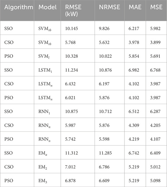
Table 6. SVM, LSTM, RNN, and EM performance evaluation of predicting models with multiple features (DHI $(Wh/m^2)$, Air Temperature (C)) optimized by meta-heuristic algorithms (SSO, CSO, PSO).

RNN₁ and ${\mathrm{R}\mathrm{N}\mathrm{N}}_n$, which are many hidden layers and a single hidden layer, respectively, are used to evaluate RNN models. The RNN are improved via optimization techniques, which show superior performance over default models. The different feature combinations used to generate EM are indicated by subscripts (a, 2, 3). The EM are refined by SSO, CSO and PSO, leading to projections of solar irradiance that are more accurate. The improved predicting models-which are refined by SSO, CSO, and PSO-show better predictive power than the default models. By efficiently navigating the model parameter space, the optimization algorithms enhance the algorithms’ capacity to identify intricate patterns in solar irradiance data. This thorough investigation of several optimization techniques and algorithms demonstrates the adaptability and potency of using metaheuristic optimization methods to improve solar predicting models.

LSTM and RNN are useful techniques that capture the intricate temporal patterns necessary for precise predictions in the field of solar radiation prediction. The LSTM architecture’s activation processes and memory cells help to learn long-term dependencies within time series data. A multi-horizon LSTM-based GHI prediction model performed very well in a recent research Mishra and Palanisamy (2018). The model’s RMSE is 18.57 W/${\mathrm{m}}^2$ overall predicted horizons. The inherent capacity of LSTM to capture temporal relationships contributes to its success in solar irradiance estimate. Similar to this, the feedback relationships between neurons and internal feedback make RNN a valuable technique. According to a research Yu et al. (2019) assessing estimates of solar radiation for 1 hour in the United States, the RNN model had the lowest RMSE of 41.37 W/${\mathrm{m}}^2$. RNN is a viable option for solar predicting due to the feedback connections that enable efficient processing of time series solar data. EM combines multiple predicting techniques and uses their combined wisdom to provide more reliable predictions. For example, EM consists of various combinations of functions related to solar radiation prediction. Many feature sets used by the team are marked with subscripts (a, 2, 3). EM have shown improved predictive capabilities after optimization with metaheuristic algorithms such as PSO, CSO, and SSO. Compared to the normal models, the optimized EMs had decreased RMSE, NRMSE, MAE, and MSE values. The efficiency of metaheuristic optimization and the adaptability of EM in integrating the complementary characteristics of several models are credited with their efficacy in increasing estimations of solar irradiation. In solar irradiance prediction, LSTM and RNN perform well because of their ability to acquire temporal dependencies. EM provides a versatile conceptualization by integrating the benefits of different techniques. After that, these learning models are refined by the application of meta-heuristic techniques, leading to accumulated efficiency and precision in solar radiation predicting tasks.

One method for dividing a dataset into a predetermined number of groups as depicted in Figure 13 using unsupervised machine learning is the grouping algorithm. To minimize the within-cluster variation, data points are repeatedly assigned to one of the k groups depending on their feature values. Each point in the graphic represents an observation from the dataset, displayed based on two chosen attributes, in the context of a pair plot with clusters. The clusters that the algorithm has allocated are denoted by different colors or markers. The x- and y-axes of each subplot in the pair plot represent distinct features, giving the data points a two-dimensional perspective. Each subplot in the pair plot represents a pairwise combination of the features in the dataset. For instance, if the dataset includes characteristics for relative humidity, air temperature, GHI, DNI, and other variables, the pair plot will display subplots for each paired combination of these features. Various colors or markers are used to symbolize different clusters; for example, blue circles may be used to symbolize Cluster 1, red triangles to symbolize Cluster 2, and so on. The algorithm’s determined centroids for each cluster may alternatively be shown on the plot as bigger or differently marked points.

Figure 13

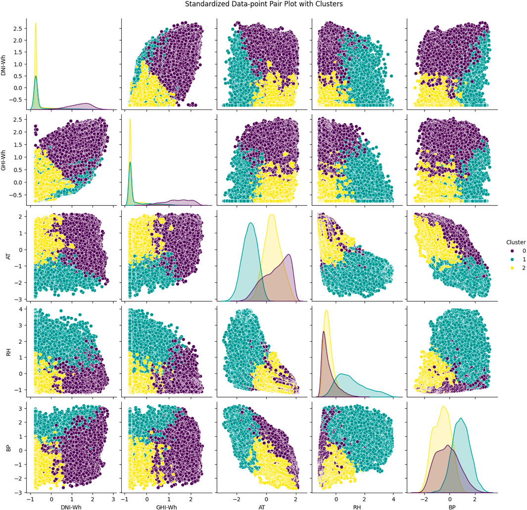
Figure 13. The pair plot, a tool for unsupervised machine learning, visualizes data grouping based on attributes like air temperature, humidity, DNI, and GHI. It shows correlations and cluster patterns, aiding in dataset understanding and improving renewable energy forecasts.

The pair plot facilitates the visualization of the degree to which the specified characteristics are used to divide the data points into clusters. While overlapping clusters may indicate that the characteristics do not give a clear distinction or that the number of clusters (k) needs to be changed, clean separation between clusters shows that the features used for the plot are successful in differentiating between various clusters. Based on the chosen attributes, each cluster collects data points that are comparable to one another, making it possible to visually evaluate the differences and similarities within and between clusters. One cluster may indicate low GHI and high relative humidity in a dataset including solar irradiance, whereas another cluster may represent high GHI and low relative humidity. The process of grouping data facilitates the discovery of underlying structures and patterns. Grouping may be used in renewable energy forecasting to classify various weather patterns, resulting in prediction models that are more precise and individualized. One may learn more about the interactions between various environmental elements and how they affect solar irradiance by examining clusters.

For clarification, let us suppose that we have four characteristics in our dataset: relative humidity (%), air temperature (C$°$), DNI (Wh/m2), and GHI (Wh/${\mathrm{m}}^2$). Six subplots would make up the pair plot, representing each potential pairing of these traits. Based on the irradiance values, points in the top-left subplot (GHI vs DNI) may be dispersed, with clusters developing where GHI and DNI have particular correlations. The GHI vs Air Temperature top-middle subplot may illustrate how GHI varies with temperature, with clusters denoting various temperature ranges connected to certain irradiance levels. GHI vs Relative Humidity, a top-right subplot that shows days with comparable irradiance and humidity characteristics as clusters, may help illustrate how GHI is affected by humidity levels.

A critical assessment of the trained Long Short-Term Memory (LSTM) model’s performance in predicting solar irradiance is given by Figure 14 titled “Predicted Hourly GHI for Test Data,” which shows a comparison between actual and predicted GHI values over 100 h Comprehension of the model’s performance in renewable energy forecasting and management requires a comprehension of this graphic. The GHI expressed in Wh/m² is plotted on the y-axis of the image, while the x-axis displays time in hours over a total of 100 h. The ground truth measurements of solar irradiance at certain timestamps are used to create the real GHI values in the dataset, which are shown by the blue line. The anticipated GHI values produced by the LSTM model, on the other hand, are shown by the red dashed line. This is because the model has been trained to recognize temporal patterns in the dataset and is based on past data.

Figure 14

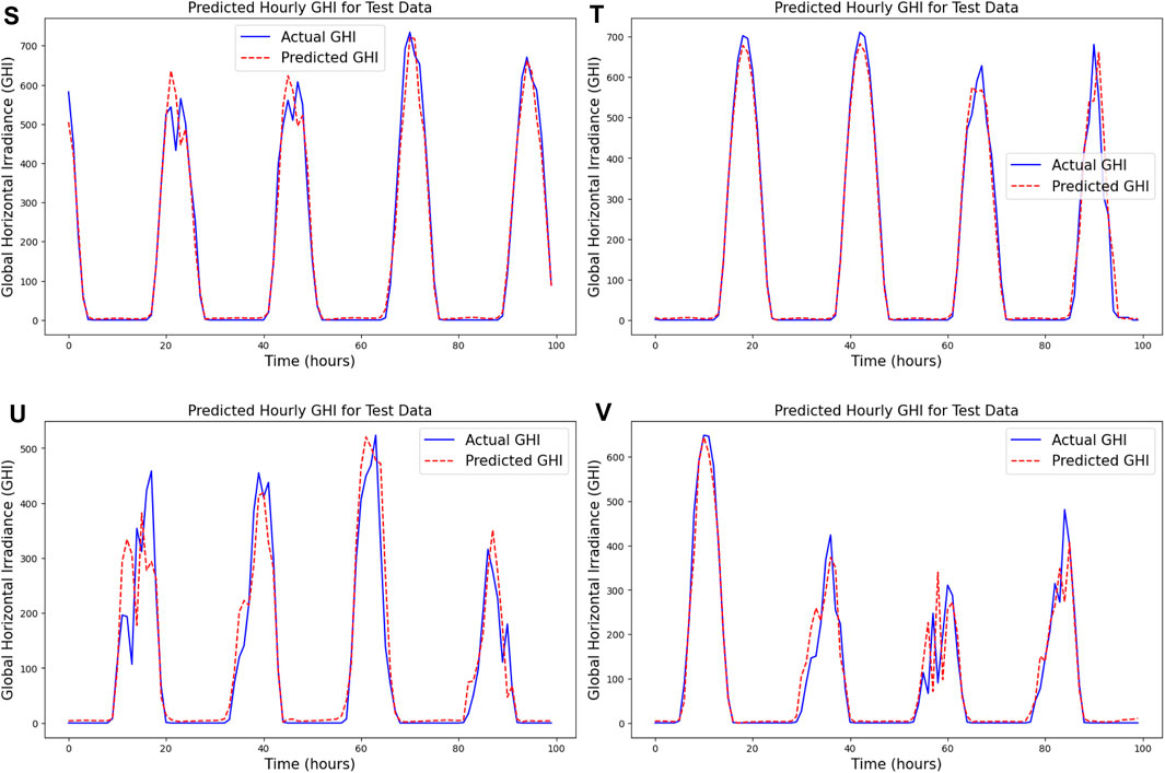
Figure 14. Effectiveness of the trained Long Short-Term Memory (LSTM) model.

As shown in Figure 14, Showcasing the effectiveness of the trained LSTM model, the figure “Predicted Hourly GHI for Test Data” compares real and predicted GHI values over 100 h. Time is shown on the x-axis in hours, while GHI is shown on the y-axis in Wh/${\mathrm{m}}^2$. The red dashed line indicates the predicted GHI values of the LSTM model, whereas the blue line displays the actual GHI values from ground truth measurements. The model’s accuracy in capturing temporal GHI trends is demonstrated by the lines’ near alignment; divergences point to problems such as abrupt weather shifts. This precise forecast is essential for improving energy storage management, guaranteeing grid stability, and optimizing solar power plants. The image illustrates how well the LSTM model predicts GHI, highlighting its potential to enhance renewable energy forecasting and management.

As predicted from solar irradiance statistics, the graphic displays a distinct diurnal pattern because of the sun’s daily cycle. The graph’s peaks mark the times of day when solar irradiance is at its maximum, usually around noon, and the troughs, where the GHI values fall to almost nil, indicate nighttime or periods of low sunshine. The blue and red lines’ near alignment indicates how well the LSTM model can represent the temporal dynamics of GHI. The model has difficulties in areas where the lines diverge, such as abrupt changes in the weather or other anomalies not found in the training set. For solar power systems to operate as efficiently as possible, accurate GHI prediction is essential. This helps with improved grid stability, energy storage management, and solar power distribution. This chart illustrates the model’s performance, which implies that LSTM networks are useful for short-term solar irradiance predictions. This may result in the more effective and dependable integration of solar energy into the electrical system. The graphic clearly illustrates how well the LSTM model captures the innate patterns of solar irradiance and shows how well it can forecast GHI with a high degree of accuracy. This performance highlights how machine learning models, especially long short-term memory models, may improve the prediction and management of renewable energy sources. By tackling the unpredictability and uncertainty related to solar electricity, these predictive models help create more reliable and sustainable energy systems.

5 Limitations and future work

In light of their narrow range of applications, current prediction systems frequently fall short of expectations. Due to transitory clouds or other meteorological phenomena, short-term variations in solar irradiance may be missed by many forecast models that rely on hourly or daily averages. This may cause forecasts of solar power in real-time to be inaccurate. Forecasting models for solar energy output usually rely on information from a small number of weather stations or satellite observations, which might not be a reliable indicator of the local circumstances for particular solar powerhouses. Disparities between anticipated and actual energy output may arise from this. Weather patterns have a significant influence on solar energy output since they may be unpredictable and substantially shift over short time intervals. It can occasionally be challenging for conventional models to accurately represent this unpredictability, especially in places with complex weather patterns. The accuracy of prediction models is largely dependent on the accessibility and dependability of past weather and solar radiation data.

In areas where this type of data is scarce or of poor quality, prediction models could not function well. Many models may not accurately represent the intricacies of real-world systems as they rely on oversimplified assumptions about how solar panels and inverters operate in various scenarios. Variations in panel deterioration over time, soiling, and shading can all have a big influence on real performance. It takes more than simply solar irradiance to predict the output of solar energy systems; it also involves understanding how this output interacts with the larger energy grid. Demand response, energy storage, and grid capacity are a few examples of factors that are frequently left out of solar forecast models, which can cause supply and demand imbalances.

Although solar energy prediction has advanced significantly, there are still several areas that need more investigation and improvement. Future research endeavors may concentrate on enhancing the temporal and geographic resolution of prediction models by the assimilation of sophisticated machine learning algorithms with high-resolution meteorological data obtained from various platforms, such as satellite observations and ground-based sensors. Short-term projections may become more accurate with the use of enhanced data assimilation techniques, which integrate historical records with real-time data. Furthermore, studies into hybrid models-which fuse statistical techniques with solar radiation physics modeling-may produce more reliable forecasts. (Figures 15, 16). Future energy planning will need to investigate how climate change affects solar energy output over the long term and incorporate this knowledge into prediction models. The advancement of increasingly complicated models that take into consideration the operational complexity of solar energy systems, such as panel deterioration, shading effects, and interactions with energy storage systems, is another area that shows promise. Ultimately, multidisciplinary research that takes into account social, environmental, and economic aspects may be useful in creating energy systems that are more robust and sustainable. These developments will help the further integration of renewable energy sources into the world energy system in addition to improving the accuracy of solar energy forecasts.

Figure 15

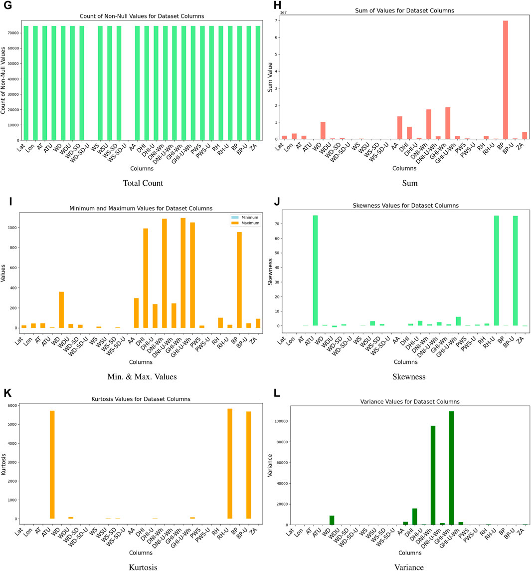
Figure 15. Basic Statistical Operations on different features.

Figure 16

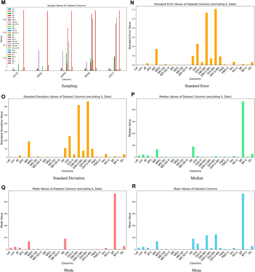
Figure 16. Basic Statistical Operations on different features.

6 Conclusion

This study delves into the intricate world of solar radiation prediction by employing advanced deep learning models (LSTM and RNN) and ensemble techniques. This work explores how these models capture temporal dynamics and leverage the collective wisdom of different learning approaches. Additionally, this study demonstrates that optimization algorithms (such as PSO, CSO, and SSO) can significantly improve the accuracy of solar activity prediction and feature extraction from time series data. Additionally, ensemble models, which are known for their flexibility, are highly effective in combining different processing capabilities to achieve robust prediction. By utilizing meta-heuristic optimization techniques, such as the proposed framework SWEPS additional potential has been unlocked, achieving even more accurate predictions. These findings are significant as they pave the way for the reliable integration of solar energy into the evolving energy landscape. They highlight the importance of accurate solar radiation estimates in meeting the increasing demand for RES. Beyond its theoretical implications, the suggested approach was successfully applied in a grid station, offering concrete proof of its usefulness in capturing solar energy. This application highlights how important this work is to enable the steady integration of solar energy into the ever-changing energy production environment. The proposed work also stresses the crucial need to assess solar radiation accurately to fulfill the growing demand for renewable energy sources.

Data availability statement

The data analyzed in this study is subject to the following licenses/restrictions: The data can be provided by KACARE. Requests to access these datasets should be directed to Atalal@qu.edu.sa.

Author contributions

TA: Conceptualization, Data curation, Formal Analysis, Funding acquisition, Investigation, Methodology, Project administration, Resources, Software, Supervision, Validation, Visualization, Writing–original draft, Writing–review and editing. SI: Conceptualization, Data curation, Formal Analysis, Funding acquisition, Investigation, Methodology, Project administration, Resources, Software, Supervision, Validation, Visualization, Writing–original draft, Writing–review and editing.

Funding

The author(s) declare that financial support was received for the research, authorship, and/or publication of this article.

Acknowledgments

The Researchers would like to thank the Deanship of Graduate Studies and Scientific Research at Qassim University for financial support (QU-APC-2024-9/1).

Conflict of interest

The authors declare that the research was conducted in the absence of any commercial or financial relationships that could be construed as a potential conflict of interest.

Publisher’s note

All claims expressed in this article are solely those of the authors and do not necessarily represent those of their affiliated organizations, or those of the publisher, the editors and the reviewers. Any product that may be evaluated in this article, or claim that may be made by its manufacturer, is not guaranteed or endorsed by the publisher.

References

Abukhait, J., Mansour, A. M., and Obeidat, M. (2018). Classification based on Gaussian-kernel support vector machine with adaptive fuzzy inference system. margin 7, 14–22. doi:10.15199/48.2018.05.03

CrossRef Full Text | Google Scholar

Al Garni, H., Kassem, A., Awasthi, A., Komljenovic, D., and Al-Haddad, K. (2016). A multicriteria decision making approach for evaluating renewable power generation sources in Saudi Arabia. Sustain. energy Technol. assessments 16, 137–150. doi:10.1016/j.seta.2016.05.006

CrossRef Full Text | Google Scholar

Almonacid, F., Rus, C., Hontoria, L., and Munoz, F. (2010). Characterisation of pv cis module by artificial neural networks. a comparative study with other methods. Renew. Energy 35, 973–980. doi:10.1016/j.renene.2009.11.018

CrossRef Full Text | Google Scholar

Almutairi, A., Nassar, M., and Salama, M. (2016). “Statistical evaluation study for different wind speed distribution functions using goodness of fit tests,” in 2016 IEEE electrical power and energy conference (EPEC) (IEEE), 1–4.

CrossRef Full Text | Google Scholar

Baseer, M. A., Meyer, J. P., Rehman, S., and Alam, M. M. (2017). Wind power characteristics of seven data collection sites in jubail, Saudi Arabia using weibull parameters. Renew. Energy 102, 35–49. doi:10.1016/j.renene.2016.10.040

CrossRef Full Text | Google Scholar

Brahma, B., and Wadhvani, R. (2020). Solar irradiance forecasting based on deep learning methodologies and multi-site data. Symmetry 12, 1830. doi:10.3390/sym12111830

CrossRef Full Text | Google Scholar

Campbell-Lendrum, D., and Prüss-Ustün, A. (2019). Climate change, air pollution and noncommunicable diseases. Bull. World Health Organ. 97, 160–161. doi:10.2471/blt.18.224295

PubMed Abstract | CrossRef Full Text | Google Scholar

Das, U. K., Tey, K. S., Seyedmahmoudian, M., Mekhilef, S., Idris, M. Y. I., Van Deventer, W., et al. (2018). Forecasting of photovoltaic power generation and model optimization: a review. Renew. Sustain. Energy Rev. 81, 912–928. doi:10.1016/j.rser.2017.08.017

CrossRef Full Text | Google Scholar

Doorga, J. R. S., Dhurmea, K. R., Rughooputh, S., and Boojhawon, R. (2019). Forecasting mesoscale distribution of surface solar irradiation using a proposed hybrid approach combining satellite remote sensing and time series models. Renew. Sustain. Energy Rev. 104, 69–85. doi:10.1016/j.rser.2018.12.055

CrossRef Full Text | Google Scholar

Duffy, A., Rogers, M., and Ayompe, L. (2015). Renewable energy and energy efficiency: assessment of projects and policies. John Wiley and Sons.

Google Scholar

Duvenhage, D. F. (2019). Sustainable future CSP fleet deployment in South Africa: a hydrological approach to strategic management. Stellenbosch: Stellenbosch University. Ph.D. thesis.

Google Scholar

Gherboudj, I., Zorgati, M., Chamarthi, P.-K., Tuomiranta, A., Mohandes, B., Beegum, N. S., et al. (2021). Renewable energy management system for Saudi Arabia: methodology and preliminary results. Renew. Sustain. Energy Rev. 149, 111334. doi:10.1016/j.rser.2021.111334

CrossRef Full Text | Google Scholar

Hochreiter, S., and Schmidhuber, J. (1997). Long short-term memory. Neural Comput. 9, 1735–1780. doi:10.1162/neco.1997.9.8.1735

PubMed Abstract | CrossRef Full Text | Google Scholar

Hoeven, M. (2015). Technology roadmap: solar photovoltaic energy. Paris, France: International Energy Agency IEA.

Google Scholar

Husein, M., and Chung, I.-Y. (2019). Day-ahead solar irradiance forecasting for microgrids using a long short-term memory recurrent neural network: a deep learning approach. Energies 12, 1856. doi:10.3390/en12101856

CrossRef Full Text | Google Scholar

Hüsken, M., and Stagge, P. (2003). Recurrent neural networks for time series classification. Neurocomputing 50, 223–235. doi:10.1016/s0925-2312(01)00706-8

CrossRef Full Text | Google Scholar

Jäger, K.-D., Isabella, O., Smets, A. H., van Swaaij, R. A., and Zeman, M. (2016). Solar energy: fundamentals, technology and systems (UIT Cambridge).

Google Scholar

Jimenez, P. A., Hacker, J. P., Dudhia, J., Haupt, S. E., Ruiz-Arias, J. A., Gueymard, C. A., et al. (2016). Wrf-solar: description and clear-sky assessment of an augmented nwp model for solar power prediction. Bull. Am. Meteorological Soc. 97, 1249–1264. doi:10.1175/bams-d-14-00279.1

CrossRef Full Text | Google Scholar

Keyno, H. S., Ghaderi, F., Azade, A., and Razmi, J. (2009). Forecasting electricity consumption by clustering data in order to decline the periodic variable’s affects and simplification the pattern. Energy Convers. Manag. 50, 829–836. doi:10.1016/j.enconman.2008.09.036

CrossRef Full Text | Google Scholar

Kumari, P., and Toshniwal, D. (2021). Deep learning models for solar irradiance forecasting: a comprehensive review. J. Clean. Prod. 318, 128566. doi:10.1016/j.jclepro.2021.128566

CrossRef Full Text | Google Scholar

Lappalainen, K., Wang, G. C., and Kleissl, J. (2020). Estimation of the largest expected photovoltaic power ramp rates. Appl. Energy 278, 115636. doi:10.1016/j.apenergy.2020.115636

CrossRef Full Text | Google Scholar

Mansour, A. M. (2018). Decision tree-based expert system for adverse drug reaction detection using fuzzy logic and genetic algorithm. Int. J. Adv. Comput. Res. 8, 110–128. doi:10.19101/ijacr.2018.836007

CrossRef Full Text | Google Scholar

Mansour, A. M., Alaqtash, M. M., and Obeidat, M. (2019). Intelligent classifiers of eeg signals for epilepsy detection. WSEAS Trans. Signal Process. 15.

Google Scholar

Mishra, S., and Palanisamy, P. (2018). “Multi-time-horizon solar forecasting using recurrent neural network,” in 2018 IEEE energy conversion congress and exposition (ECCE) (IEEE), 18–24.

CrossRef Full Text | Google Scholar

Ouarda, T. B., Charron, C., Shin, J.-Y., Marpu, P. R., Al-Mandoos, A. H., Al-Tamimi, M. H., et al. (2015). Probability distributions of wind speed in the uae. Energy Convers. Manag. 93, 414–434. doi:10.1016/j.enconman.2015.01.036

CrossRef Full Text | Google Scholar

Pedregal, D. J., and Trapero, J. R. (2010). Mid-term hourly electricity forecasting based on a multi-rate approach. Energy Convers. Manag. 51, 105–111. doi:10.1016/j.enconman.2009.08.028

CrossRef Full Text | Google Scholar

Perez, R., Lorenz, E., Pelland, S., Beauharnois, M., Van Knowe, G., Hemker, Jr. K., et al. (2013). Comparison of numerical weather prediction solar irradiance forecasts in the us, Canada and europe. Sol. Energy 94, 305–326. doi:10.1016/j.solener.2013.05.005

CrossRef Full Text | Google Scholar

Salah, I. (1997) “Inventory and assessment of solar-cells systems in Libya,” in 6th series of desert study. Paris, France: issued by Arab Centre for Research and Development of saharian communites.

Google Scholar

Srivastava, S., and Lessmann, S. (2018). A comparative study of lstm neural networks in forecasting day-ahead global horizontal irradiance with satellite data. Sol. Energy 162, 232–247. doi:10.1016/j.solener.2018.01.005

CrossRef Full Text | Google Scholar

Tang, C.-Y., Chen, Y.-T., and Chen, Y.-M. (2015). Pv power system with multi-mode operation and low-voltage ride-through capability. IEEE Trans. Industrial Electron. 62, 7524–7533. doi:10.1109/tie.2015.2449777

CrossRef Full Text | Google Scholar

Wojtkiewicz, J., Hosseini, M., Gottumukkala, R., and Chambers, T. L. (2019). Hour-ahead solar irradiance forecasting using multivariate gated recurrent units. Energies 12, 4055. doi:10.3390/en12214055

CrossRef Full Text | Google Scholar

Yang, C., Thatte, A. A., and Xie, L. (2014). Multitime-scale data-driven spatio-temporal forecast of photovoltaic generation. IEEE Trans. Sustain. Energy 6, 104–112. doi:10.1109/tste.2014.2359974

CrossRef Full Text | Google Scholar

Yu, Y., Cao, J., and Zhu, J. (2019). An lstm short-term solar irradiance forecasting under complicated weather conditions. IEEE Access 7, 145651–145666. doi:10.1109/access.2019.2946057

CrossRef Full Text | Google Scholar

Zang, H., Cheng, L., Ding, T., Cheung, K. W., Wang, M., Wei, Z., et al. (2020a). Application of functional deep belief network for estimating daily global solar radiation: a case study in China. Energy 191, 116502. doi:10.1016/j.energy.2019.116502

CrossRef Full Text | Google Scholar

Zang, H., Liu, L., Sun, L., Cheng, L., Wei, Z., and Sun, G. (2020b). Short-term global horizontal irradiance forecasting based on a hybrid cnn-lstm model with spatiotemporal correlations. Renew. Energy 160, 26–41. doi:10.1016/j.renene.2020.05.150

CrossRef Full Text | Google Scholar

Zeng, Z., Li, H., Tang, S., Yang, H., and Zhao, R. (2016). Multi-objective control of multi-functional grid-connected inverter for renewable energy integration and power quality service. IET Power Electron. 9, 761–770. doi:10.1049/iet-pel.2015.0317

CrossRef Full Text | Google Scholar

Zhang, X., Li, Y., Lu, S., Hamann, H. F., Hodge, B.-M., and Lehman, B. (2018). A solar time based analog ensemble method for regional solar power forecasting. IEEE Trans. Sustain. Energy 10, 268–279. doi:10.1109/tste.2018.2832634

CrossRef Full Text | Google Scholar

Zhang, Y., Beaudin, M., Taheri, R., Zareipour, H., and Wood, D. (2015). Day-ahead power output forecasting for small-scale solar photovoltaic electricity generators. IEEE Trans. Smart Grid 6, 2253–2262. doi:10.1109/tsg.2015.2397003

CrossRef Full Text | Google Scholar

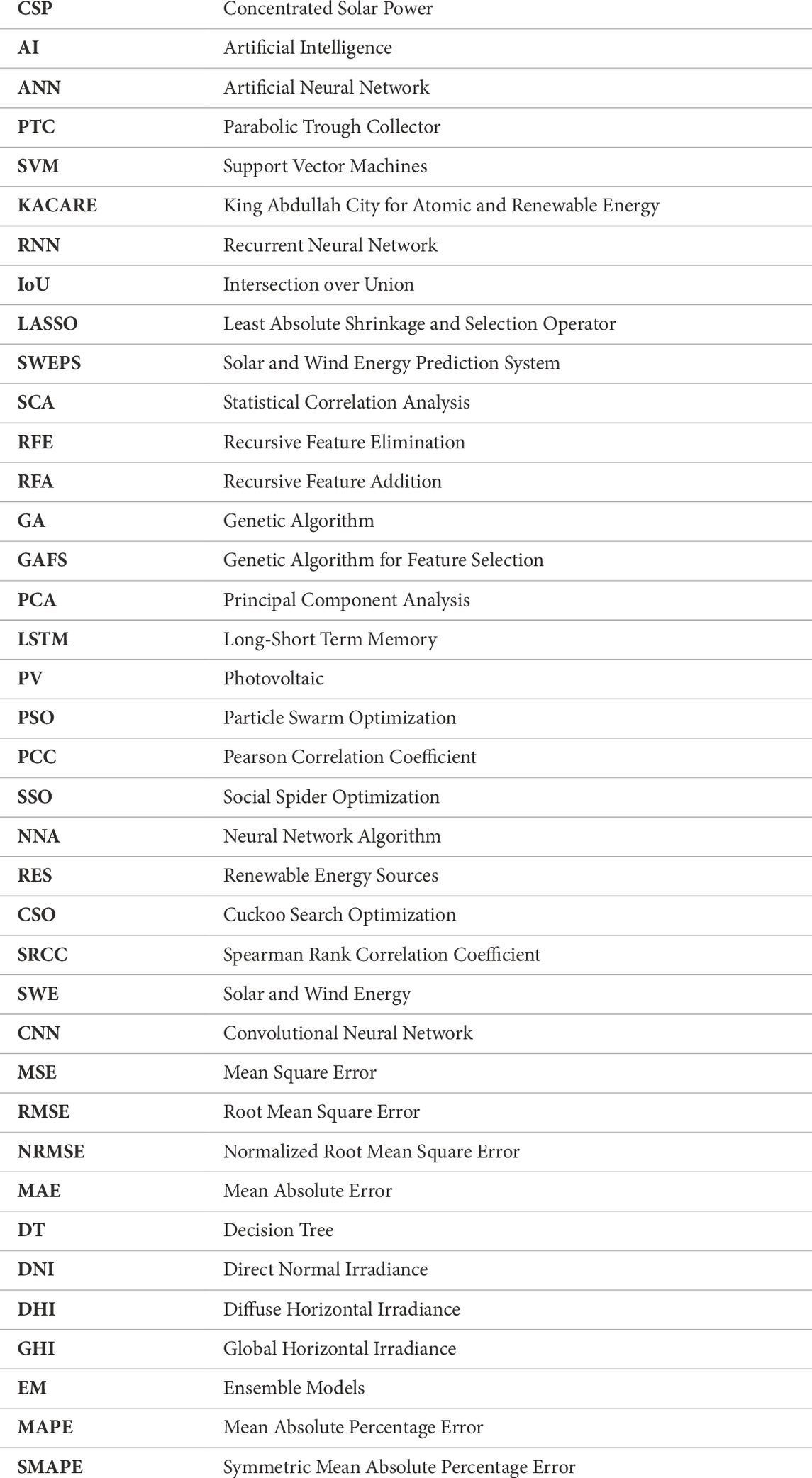
Glossary