Bayesian regression modeling and inference of energy efficiency data: the effect of collinearity and sensitivity analysis

The majority of research predicted heating demand using linear regression models, but they did not give current building features enough context. Model problems such as Multicollinearity need to be checked and appropriate features must be chosen based on their significance to produce accurate load predictions and inferences. Numerous building energy efficiency features correlate with each other and with heating load in the energy efficiency dataset. The standard Ordinary Least Square regression has a problem when the dataset shows Multicollinearity. Bayesian supervised machine learning is a popular method for parameter estimation and inference when frequentist statistical assumptions fail. The prediction of the heating load as the energy efficiency output with Bayesian inference in multiple regression with a collinearity problem needs careful data analysis. The parameter estimates and hypothesis tests were significantly impacted by the Multicollinearity problem that occurred among the features in the building energy efficiency dataset. This study demonstrated several shrinkage and informative priors on likelihood in the Bayesian framework as alternative solutions or remedies to reduce the collinearity problem in multiple regression analysis. This manuscript tried to model the standard Ordinary Least Square regression and four distinct Bayesian regression models with several prior distributions using the Hamiltonian Monte Carlo algorithm in Bayesian Regression Modeling using Stan and the package used to fit linear models. Several model comparison and assessment methods were used to select the best-fit regression model for the dataset. The Bayesian regression model with weakly informative prior is the best-fitted model compared to the standard Ordinary Least Squares regression and other Bayesian regression models with shrinkage priors for collinear energy efficiency data. The numerical findings of collinearity were checked using variance inflation factor, estimates of regression coefficient and standard errors, and sensitivity of priors and likelihoods. It is suggested that applied research in science, engineering, agriculture, health, and other disciplines needs to check the Multicollinearity effect for regression modeling for better estimation and inference.

1 Introduction

Several studies used regression models to predict the electric energy consumption and efficiency of office or residence buildings without checking Multicollinearity effects in a frequentist statistical approach (Baranova et al., 2017; Reim et al., 2017; Taskin et al., 2022; Neubauer et al., 2024). To make sure that investments in energy conservation measures (ECMs) and the development of new energy-efficient buildings provide the anticipated and promised performance, reliable estimating techniques are required to assess the effects of various features. The standard linear regression approach has limitations in estimating and inferring energy efficiency data having collinear features (Moletsane et al., 2018; Mummolo and Peterson, 2018; Tahmasebinia et al., 2023; Ahmadi, 2024; Kaczmarczyk, 2024).

The conventional method for estimating energy efficiency involves using a linear regression model. However, only partially addressed the statistical issues described for the linear regression approach and the potential Multicollinearity issue due to the high correlation between building energy efficiency (Moletsane et al., 2018; Tahmasebinia et al., 2023; Ahmadi, 2024; Kaczmarczyk, 2024). Bayesian inference has various applications in science, engineering, and social sciences. Model parameters are assumed to be constant in traditional frequentist inference (Nithin, 2023). Using existing data and prior knowledge of population parameters, Bayesian statistics is a statistical tool that may generate estimates via the posterior distribution. For both experimental and applied studies, one of the most widely used statistical techniques is Bayesian Multiple Regression (BMR) analysis. Nevertheless, associated predictor variables and their collinearity effects are frequently a source of worry in the statistical inference of regression estimates (Farrar and Glauber, 1967). Strong correlation among independent variables in multiple linear regression models leads to high Standard Errors (SE) of the regression coefficients, known as the Multicollinearity problem (Willis and Perlack, 1978). Bayesian inference in multiple linear regression analysis considered estimators for testing simple hypotheses concerning the regression coefficients (Wu et al., 2023). Bayesian interval estimation (credible intervals) can be formulated using prior information of various kinds incorporated in the analysis (Assaf and Tsionas, 2021b). Due to efficiency in computing, accuracy in the estimate, and variable selection, Bayesian shrinkage and non-informative priors have attracted much interest recently.

Many characteristics of building energy efficiency are correlated with the heating load as well as with each other (Jammulamadaka et al., 2022). Potential Multicollinearity issue due to the high correlation between energy efficiency features provides biased estimates and untruthful inferences. To achieve optimal energy efficiency feature selection is required with appropriate methods of analysis. To reduce the detrimental effects of Multicollinearity on the estimations of energy efficiency, biased regression procedures have been developed.

The main consequence of Multicollinearity in statistical estimation and inference is to inflate the SE of some or all regression coefficients of the fitted model (Kim, 2019); which leads to failure to reject the null hypothesis on the significance of the regression coefficient and wider confidence interval. The type II error rate (lowering power) of the parameter hypothesis tests increased due to exaggerated SE and confidence intervals of the estimated model parameters. Multicollinearity has statistical repercussions, such as exaggerated standard errors that make it challenging to assess individual regression coefficients in hypothesis testing (Assaf and Tsionas, 2021a).

The other consequence is that the posterior distribution would seem to recommend that none of the variables is reliably related to the outcome variable, even if all predictor variables are strongly related to the outcome. In contrast to statistical inference on the regression coefficients, Multicollinearity does not impact the model’s overall fit to the observed response variable data and prediction (Alin, 2010). The issues of autocorrelation, Multicollinearity, and heteroscedasticity plague the majority of econometric models. The assumptions of the standard regression model are not always met in real-world situations (Youssef, 2022).

The effects of Multicollinearity can be either numerical or statistical in such a way that the statistical consequences of Multicollinearity include difficulties in testing the individual parameters of regression coefficients due to inflated standard errors. Due to large standard errors, a large confidence region may arise. If the researcher(s) need to explain the effect of individual regression coefficients on Y, the statistical consequence of Multicollinearity will cause trouble, because this effect cannot be separated. Therefore, we may be unable to declare the significance of the predictor (X) even though it has a strong relationship with the targeted outcome (dependent) variable (Y). Moreover, the Ordinary Least Squares Estimates (OLSE) may be sensitive to small changes in the values of explanatory variables. On the other hand, numerical consequences of Multicollinearity include difficulties in computer calculations due to numerical instability. In extreme cases, the computer may try to divide by zero and thus fail to complete the analysis. Or even worse, the computer may complete the analysis but then report meaningless, widely incorrect numbers.

Multicollinearity can be identified using a correlation matrix or Variance Inflation Factor (VIF) of features that can predict the outcome variable with a high R-squared value demonstrating a strong linear relationship (Alin, 2010). Regression coefficients in multiple regression models with a VIF of more than 10 are not robustly computed when Multicollinearity is present (Shrestha, 2020).

A study has used the prediction of heating and cooling loads using partial least squares towards efficient residential building design without checking assumptions of the classical approaches (Kavaklioglu, 2018). Many researchers and statisticians are reluctant to apply Bayesian statistical approaches since they find it difficult to draw conclusions based on their prior opinions (Sinay and Hsu, 2014). Bayesian inference of the posterior is strongly influenced by the prior information (Oluwadare, 2021). Utilizing prior knowledge in addition to sample data is one of the primary benefits of Bayesian techniques. Adding more prior information can be an alternate strategy to lessen the uncertainty caused by collinearity. Among the several methods to address the problem of Multicollinearity were the use of shrinkage priors and associated algorithms such as a ridge, LASSO (Least Absolute Shrinkage and Selection Operator), or elastic net regression. Imposing shrinkage priors mitigates the collinearity problem by sifting the likelihood surface to create a posterior distribution, which divides up the pertinent likelihood data among the subset modes (Mahajan et al., 1977; Garg, 1984; Ročková and George, 2014; Zhang et al., 2022).

Energy efficiency and power-related datasets are the most correlated attributes to understand what to exclude from regression to avoid Multicollinearity problems. To design buildings that follow certain standards architects and engineers need to identify which parameters will significantly influence future energy demand (Sekhar Roy et al., 2018).

Multicollinearity decreases the statistical power of the regression model by reducing the precision of the calculated regression coefficients and making the model extremely sensitive to even tiny changes in the observed values and model (Ročková and George, 2014). A sensitivity analysis evaluates the analysis carried out using Ordinary Least Squares (OLS) regression and Bayesian regression analysis in which Bayesian shrinkage priors were changed in the regression model (Piironen and Vehtari, 2017b; Ackermann, 2019; Kim et al., 2019). Sensitivity analysis is used to evaluate the estimation and influence of regression results on changes in different modeling approaches (Seltzer, 1993). Having strongly correlated predictors can increase the uncertainty of the posterior distributions of the regression coefficients (Van de Schoot and Depaoli, 2014). On the contrary, using the earlier distribution in Bayesian analyses can particularly come to the rescue because it makes it much less possible for the posteriors to have an extraordinarily huge posterior mean and standard deviation. To estimate the Heating Load (HL) and Cooling Load (CL) of the energy-effectual housing structures, Bui et al. (2019), employed Artificial Neural Networks (ANNs). To achieve this, a suitable data set was supplied that comprises the heating load and the cooling load with the relevant factors, relative compactness, surface area, wall area, roof area, overall height, orientation, glazing area, and distribution of the glazing area.

In practical Bayesian statistics, multiple regression, Bayesian networks, and artificial neural networks were used for prediction (Felipe et al., 2015). An artificial neural network with Bayesian regularization modeling was used to assess the performance of electronic components over their lifetimes in four different scenarios. The findings showed that there was a direct relationship between the reliability parameters examined in all scenarios and an increase in the Mean Time Between Failures value appeared for each scenario (Çolak et al., 2023); and ANNs with Bayesian regularization are an effective and potent mathematical technique for evaluating a lifetime model’s dependability (Sindhu et al., 2023).

Several studies demonstrated the superiority of the Bayesian approach over the frequentist approach of the multiple linear regression model in identifying the predictors for the outcome variable (Zianis et al., 2016; Gebrie, 2021; Tanoe et al., 2021; Vijayaragunathan et al., 2023). But what distinguishes this study from others is the way it takes into account the Multicollinearity effect and applies multiple prior distributions or beliefs to evaluate sensitivity in Bayesian regularization of regression parameters.

According to Pesaran and Smith (2019), in scenarios of exact and highly collinear predictors, the asymptotic behavior of the posterior estimate, and the accuracy of the parameters of a linear regression model are investigated. In both scenarios, even when the sample size is large enough, the estimates of the posterior distribution are still sensitive to the selection of prior distribution, and the precision increases more slowly than the sample size.

Figuring out how sensitive the posterior is to changes in the prior distribution and the likelihood is a crucial step in the Bayesian workflow. Sensitivity can be distinguished using power-scaling the prior or likelihood (Kallioinen et al., 2024). The Ordinary Least Squares (OLS) method is distribution-free because it does not utilize any distribution of the data. Without making certain assumptions about the probability model that underlies the data, it is impossible to draw any statistical inferences about the slope, intercept, or prediction from the OLS estimates. Thus, all datasets must mitigate Multicollinearity in Bayesian inference and select the appropriate predictive model. This manuscript tried to model the standard OLS regression and four distinct Bayesian regression models, with several shrinkage or regularized prior distributions, for the real dataset which showed collinearity.

The existing and recommended solutions to cover and reduce the Multicollinearity in the presence of highly correlated independent variables are increasing sample size to strengthen the statistical power, omission of one or more of the affected variables from the analysis, combining the strongly correlated variables into a single composite score or switching to more adequate modeling approaches able to handle correlated variables such as principal component analysis (PCA) or partial least-squares (PLS) regression and using regularization methods such as RIDGE and LASSO or Bayesian regression (Voss, 2004; Jaya et al., 2019). However, the omission of one variable or the creation of a composite score can be done for bivariate correlation but leads to different interpretations of the model. Moreover, switching to models that can handle inter-related explanatory variables does not provide the statistical hypothesis test and the hypothesis testing in the regression model has been not solved yet. The method must be able to obtain the parameter estimates with a high level of precision and also facilitate the hypothesis test of regression parameters simultaneously (Pesaran and Smith, 2019). We proposed the Bayesian regression method with weakly informative and shrinkage (regularized) priors as an alternative solution. The Monte Carlo simulation revealed that the Bayesian method solves hypothesis testing in regression analysis with interpretability in the Multicollinearity problem effectively. Therefore, the main purpose of this study is to fit multiple linear regression models using OLS and the Bayesian approach with different shrinkage prior distributions for sensitivity analysis of the priors and to find the best-fitted model for the collinear data.

2 Materials and methods

2.1 Multiple linear regression (classical versus bayesian)

In classical statistical theory, unlike random effect models, which use a random sample from the population for group mean calculations, fixed effect models use regression analysis where group means are fixed (Mummolo and Peterson, 2018). Here, the fixed effect model is used as a linear regression model with one outcome or dependent variable $\left(Y\right)$ and $\mathit{p}$ input or independent variables $\left(X_1,X_2,X_2,\dots ,X_p\right)$, as multiple regression in Eqs 1, 2, can be expressed as follows.

$Y={\beta }_0+{\beta }_1{X}_1+{\beta }_2{X}_2+{\beta }_3{X}_3+\dots +{\beta }_p{X}_p+\epsilon (1)$

$\mathit{Y}=\mathit{X}\mathit{\beta }+\mathit{\epsilon }(2)$

where $Y$ is a target or outcome variable with a dimension of $\left(n\times 1\right)$.

$X$ is a design matrix of input variables with a constant column of dimension $\left(n\times \left(p+1\right)\right)$.

$\beta$ is a vector of regression parameters or coefficients having $\left(\left(p+1\right)\times 1\right)$ dimension.

$\epsilon$ is a vector of error terms with a dimension of $\left(n\times 1\right)$ (Mettle et al., 2016).

In matrix notation, multiple linear regression can be rewritten as Eq. 3.

$\mathit{Y}=\left[\begin{array}{c}{y}_1\\ y_2\\ y_3\\ \dots \\ y_n\end{array}\right]\mathit{X}=\left[\begin{array}{c}\begin{array}{ccc}1& x_{11}& \dots \\ 1& x_{21}& \cdots \\ 1& x_{31}& \dots \end{array}\begin{array}{c}{x}_{1p}\\ x_{2p}\\ x_{3p}\end{array}\\ \begin{array}{cc}\begin{array}{ccc}⋮& \dots & \ddots \end{array}& ⋮\end{array}\\ \begin{array}{ccc}1& \begin{array}{cc}{x}_{n1}& \dots \end{array}& x_{np}\end{array}\end{array}\right]\mathit{\beta }=\left[\begin{array}{c}{\beta }_0\\ {\beta }_1\\ {\beta }_{\mathbf{2}}\\ {\beta }_{\mathbf{3}}\\ ⋮\\ {\beta }_{\mathit{p}}\end{array}\right]\mathit{\epsilon }=\left[\begin{array}{c}{\epsilon }_1\\ {\epsilon }_2\\ {\epsilon }_{\mathbf{3}}\\ ⋮\\ {\epsilon }_n\end{array}\right](3)$

From the general multiple linear regression model in Eq. 2 of $\mathit{p}$ input variables on $\mathit{n}$ sample data, the solution derived from Eq. 4.

${\mathit{X}}^T\mathit{X}\widehat{\mathit{\beta }}={\mathit{X}}^{\mathit{T}}\mathit{y}(4)$

summarizes $\mathit{p}$ normal equations in the $\mathit{k}$ components of $\widehat{\mathit{\beta }}$. Two parameters have to be estimated, $\mathit{\beta }$ and ${\sigma }^2$ and $y\sim N\left(\mathit{X}\mathit{\beta },{\sigma }^2\mathit{I}\right)$. Solving the normal equations by elimination, the vector of regression coefficients shown in Eq. 5 can be computed as follows:

$\widehat{\mathit{\beta }}={\left({\mathit{X}}^T\mathit{X}\right)}^{-1}{\mathit{X}}^{\mathit{T}}\mathit{y}(5)$

with the vector of residuals shown in Eq. 6;

$\widehat{\mathit{e}}\equiv \left(\mathit{y}-\mathit{X}\widehat{\mathit{\beta }}\right)(6)$

However, if more parameters to be estimated are available than observations $\left(\mathit{p}>\mathit{n}\right)$, or if $\mathit{p}\le \mathit{n}$, but some of the underlying explanatory variables are perfectly correlated, there will be Multicollinearity $\left(\left|{\mathit{X}}^T\mathit{X}\right|=\mathbf{0}\right)$ and an inverse of ${\mathit{X}}^T\mathit{X}$ will not exist (Frost, 2019). In either case, there are an infinite number of solutions to Eq. 4, and unless extraneous variables are eliminated by deleting the corresponding rows and columns of ${\mathit{X}}^T\mathit{X}$ (and deleting the corresponding elements of $\left.\mathit{\beta }\right)$, or prior information is brought to bear on the problem in some form to eliminate the ambiguity. A unique solution cannot be obtained (Ullah, 2021).

An alternative approach to estimating and deducing regression model parameters is provided by Bayesian linear regression. The Bayesian method has prior, likelihood, and posterior distributions. The posterior is created by combining the sample data with the prior according to Bayes’ theorem. The normally distributed error assumption, denoted by $\epsilon \sim N\left(0,{\sigma }^2\right)$, is present in the linear regression model that uses the OLS estimation method. In the linear regression model using the OLS estimation method, there is a normally distributed error assumption that is $\epsilon \sim N\left(0,{\sigma }^2\right)$. Since the error term is normally distributed, the three variables $\mathit{Y}/\mathit{X}$, $\mathit{\beta },$ ${\mathit{\sigma }}^2$ have a normal distribution as does the error (Miroshnikov et al., 2015; Samira, 2023). β and σ2 are the vectors of regression coefficient and residual parameters in the standard regression approach having a normal distribution based on the error term. However, the Bayesian concept thought of these parameters as random variables having distinct distributions with hyper-parameters. In the Bayesian context the distribution β of depend on the choice of the prior distribution, so it will not necessarily be a normal distribution. In Bayesian inference, parameters are considered random variables because their values are uncertain; it means the value is not a single value. The main difference between classical and Bayesian statistics is that in frequentist approaches, parameters are considered fixed and unknown constants that can be estimated from the data. In contrast, Bayesian approaches treat parameters as random variables with their distributions, reflecting uncertainty about their values (Nithin, 2023). This allows for the incorporation of prior knowledge or beliefs about parameters in the Bayesian approach, which gets updated with new data through Bayes’ theorem, leading to a posterior distribution that expresses updated beliefs about the parameters’ values. Thus, $\left(\mathit{Y}/\mathit{X},\mathit{\beta }{,\mathit{\sigma }}^2\right)\sim N\left(\mathit{X}\mathit{\beta },{\sigma }^{\mathbf{2}}\right)$ and the joint probability density function (pdf) of these variables can be written as:

$p\left(\mathit{Y}/\mathit{X},\mathit{\beta }{,\mathit{\sigma }}^2\right)=\frac{1}{\sqrt{2\pi {\sigma }^2}}\mathit{exp}\left[-\frac{1}{2{\sigma }^2}{\left(\mathit{Y}/\mathit{X},\mathit{\beta }{,\mathit{\sigma }}^2\right)}^T\left(\mathit{Y}/\mathit{X},\mathit{\beta }{,\mathit{\sigma }}^2\right)\right](7)$

The likelihood function of these variables is derived from the above probability density function (pdf) and can be expressed as Eqs 8, 9;

$p\left(\mathit{Y}/\mathit{X},\mathit{\beta }{,\mathit{\sigma }}^2\right)={\displaystyle \prod _{i=1}^n}\frac{1}{\sqrt{2\pi {\sigma }^2}}\mathit{exp}\left[-\frac{1}{2{\sigma }^2}{\left(\mathit{Y}/\mathit{X},\mathit{\beta }{,\mathit{\sigma }}^2\right)}^T\left(\mathit{Y}/\mathit{X},\mathit{\beta }{,\mathit{\sigma }}^2\right)\right]={\left({\sigma }^2\right)}^{-n/2}\mathit{exp}\left[-\frac{1}{2{\sigma }^2}{\left(\mathit{Y}/\mathit{X},\mathit{\beta }{,\mathit{\sigma }}^2\right)}^T\left(\mathit{Y}/\mathit{X},\mathit{\beta }{,\mathit{\sigma }}^2\right)\right](8)$

$p\left(\mathit{Y}/\mathit{X},\mathit{\beta }{,\mathit{\sigma }}^2\right)\propto {\left({\sigma }^2\right)}^{\raisebox{1ex}{$-\nu $}\!\left/ \!\raisebox{-1ex}{$2$}\right.}\left[\frac{\nu s^2}{2{\sigma }^2}\right]\times {\left({\sigma }^2\right)}^{-n/2}\mathit{exp}\left[-\frac{1}{2{\sigma }^2}{\left(\mathit{Y}/\mathit{X},\mathit{\beta }{,\mathit{\sigma }}^2\right)}^T\left(\mathit{Y}/\mathit{X},\mathit{\beta }{,\mathit{\sigma }}^2\right)\right](9)$

Regression parameter estimates can be obtained using the Bayesian technique by iterating in the marginal posterior. As shown in Eq. 10, the posterior distribution can be obtained by multiplying the likelihood function by the prior information (Gelman et al., 2013).

$Posterior\propto Prior\times Likelihood$

$p\left(\mathit{\beta }{,\mathit{\sigma }}^2/\mathit{Y},\mathit{X}\right)\propto p\left(\mathit{Y}/\mathit{X},\mathit{\beta }{,\mathit{\sigma }}^2\right)\times p\left({\mathit{\sigma }}^2\right)\times p\left(\mathit{\beta }/{\mathit{\sigma }}^2\right)(10)$

Markov Chain Monte Carlo (MCMC) is a technique that can estimate regression model parameters using a Bayesian approach. The most common MCMC algorithms used in Bayesian estimation are Gibbs sampling, Metropolis-Hastings, and Hamiltonian Monet Carlo approximations.

2.2 Estimation and inference in Bayesian multiple regression

In the Bayesian framework, prior distributions to $\mathit{\beta }$ and ${\mathit{\sigma }}^2$ need to be assigned (Miroshnikov et al., 2015). For convenience, Bayesian models use precision $\left(\tau \right)$ rather than variance $\left({\sigma }^2\right)$ as specified in Eqs 7, 11. Considering this parameterization, a Bayesian Multiple Regression model assumes,

$\begin{array}{c}\left(\mathit{Y}/\mathit{\beta },\tau \right)\sim N_n\left(\mathit{X}\mathit{\beta },\frac{1}{\mathit{\tau }}\mathit{I}\right),\\ \frac{\mathit{\beta }}{\mathit{\tau }}\sim N_{\mathit{p}+\mathbf{1}}\left(\varphi ,\frac{1}{\mathit{\tau }}\mathit{V}\right),\\ \mathit{\tau }\sim \mathit{D}\left(\alpha ,\delta \right)\end{array}(11)$

where $\alpha$ and $\delta$ are hyper-parameters of the prior $\mathit{D}$.

A Bayesian point estimate of ${\beta }_i$ is its posterior mean ${\varphi }_{*i}$ and a $100\left(1-\omega \right)\%$ Bayesian credible interval for ${\beta }_i$ is ${\varphi }_{*i}+t_{\raisebox{1ex}{$w$}\!\left/ \!\raisebox{-1ex}{$2$}\right.,n+2\alpha }{w}_{*ii}$, where ${\varphi }_{*i}$ is the $i^{th}$ element of ${\mathit{\varphi }}_{*}={\left({\mathit{V}}^{-\mathbf{1}}+{\mathit{X}}^{\mathit{T}}\mathit{X}\right)}^{-\mathbf{1}}\left({\mathit{V}}^{-\mathbf{1}}\mathit{\varphi }+{\mathit{X}}^{\mathit{T}}\mathit{y}\right)$, $w_{*ii}$ is the $i^{th}$ diagonal element of ${\mathit{W}}_{*}=\left(\frac{{\left(\mathit{y}-\mathit{X}\mathit{\varphi }\right)}^{\mathit{T}}{\left(\mathit{I}+\mathit{X}\mathit{V}{\mathit{X}}^{\mathit{T}}\right)}^{-\mathbf{1}}\left(\mathit{y}-\mathit{X}\mathit{\varphi }\right)+\mathbf{2}\mathit{\delta }}{\mathit{n}+\mathbf{2}\mathit{\alpha }}\right){\left({\mathit{V}}^{-\mathbf{1}}+{\mathit{X}}^{\mathit{T}}\mathit{X}\right)}^{-\mathbf{1}}.$

To evaluate the null hypothesis test: $H_0:{\beta }_i>{\beta }_{i0}$, the probability can be calculated as $P\left(t_{\left(n+2\alpha \right)}>\frac{{\beta }_{i0}-{\varphi }_{*i}}{w_{*ii}}\right)$. This expletory index of features in Bayesian inference that is used as the numeric equivalent of P-value in classical statistics was computed as Probability of Direction (PD) using the BRMS package. A hypothesis is considered more believable when the higher its probability (Kruschke and Liddell, 2018).

Prior information can be introduced from the sampling theory viewpoint by imposing side situations on the regression parameters and using the formalism of the general inverse (Soofi, 1990). Prior information enters the problem for a Bayesian when he assesses an informative prior distribution for the regression parameters (Leamer, 1973). However, using diffuse (non-informative) prior will not extricate the analysis from the Multicollinearity problem since such priors do not add enough information.

The parameters that need to be estimated have a probability distribution known as the prior distribution (Consonni et al., 2018). At the same time, the likelihood is a combined distribution of the necessary data parameters, even though it is connected to the probability distribution of the observational and posterior distributions. The prior is decided earlier than the measurement facts are held, so the likelihood function is frequently articulated as a confirming feature of the prior knowledge. Inference on Bayesian models and posterior distributions was done using the “Bayes test” of the R package.

Model selection using the Bayes factor and Bayesian hypothesis testing were carried out by Andraszewicz et al. (2015). An expanded example of using hierarchical regression, which is based on experiment study design in management, the usage of Bayes factors is demonstrated. Reporting and characterizing of the fitted models and posterior distributions can be done using the Highest Density Interval (HDI), credible interval, and the Region of Practical Equivalence (ROPE) percentage, or Equivalence Test functions to check whether the Bayesian regression can be considered non-negligible. The credible interval also known as the Bayesian 95% confidence interval can be interpreted as given the evidence presented by the observed data, the Bayesian Credible Interval (BCrI) contains a 95% chance of holding the true (unknown) value (Hespanhol et al., 2019).

In this study, the Hamiltonian Monte Carlo (HMC) algorithm of Bayesian Regression Models in STAN (BRMS) of the R package has been used to fit Bayesian Regression Models (BRM) and the package “lm” for the classical regression model. Stan makes use of a variation of a No-Uturn Sampler (NUTS) to discover the goal parameter area and provide output. Afterward, until the burn-in requirements are satisfied, the iteration procedure estimates the parameters. The classical multiple linear regression with OLS estimation, Bayesian multiple regression with ridge prior (Model 1), Bayesian multiple regression with Horseshoe prior (Model 2), Bayesian multiple regression with R-Square-Induced Dirichlet Decomposition (R2-D2) prior (Model 3), and Bayesian multiple linear regression with a weakly informative prior (Model 4) from the BRMS package in Stan were fitted.

The scale reduction factor (Rhat) is the root mean square of the separate within-chain standard deviations divided by the standard deviation of the individual relevant scalar measures of interest from all the chains combined. We do not experience any MCMC convergence issues when this number is around 1. For most purposes, an Effective Sample Size (ESS) of more than 1,000 is sufficient to generate stable estimates, even though the ESS should be as large as feasible (Bürkner, 2017). In terms of estimate power, the ESS (Bulk_ESS and Tail_ESS) represents the number of independent samples having the same value as the N auto-correlated samples. “How much independent information there is in auto-correlated chains” is what it measures (Kruschke and Liddell, 2018).

2.3 Types of priors

A prior is a statistical distribution that can be employed to represent the degree of (un)certainty in a population parameter. The posterior, used to produce Bayesian inference, is obtained by weighting the distribution after the prior and likelihood are merged in the Bayesian estimating process (Van de Schoot and Depaoli, 2014).

2.3.1 Non-informative prior

The dimensions of this kind of prior are not well understood. Laplace, Bayes, Jeffreys, and Gauss invented the non-informative prior (Grzenda, 2016). Although Jeffreys’s prior is frequently criticized in multivariate contexts, it was universally accepted in univariate cases (Lemoine, 2019). From a Bayesian point of view, using a (improper) uniform prior yields matching results with standard OLS estimates in the sense that posterior quantiles agree with one-sided confidence bounds. For this and several other reasons, the uniform prior is often considered objective or non-informative.

2.3.2 Informative prior

The informative prior, also known as the prior where information is available about the prior distribution and summarizes the evidence about the parameters concerned from many sources, is referred to as the prior where information is available about the prior distribution (Nasional et al., 2019). Stan considers a Student-t distribution with location 0, the user-specified degrees of freedom, $d_t$, and a reasonable $s_t$ that can be written as $t\sim Student\_t\left(d_t,0,s_t\right)$. In this manuscript, weakly informative priors such as student_t (3, 0, 2) and the ridge prior as Gaussian (0, 1) were selected for fixed effect parameters $\mathit{\beta }$.

2.3.3 Shrinkage priors

Defining a joint distribution for the unobserved regression coefficients is necessary for prior distributions for multidimensional linear regression (Piironen and Vehtari, 2017a). Shrinkage priors such as Bayesian lasso prior (Oluwadare, 2021), spike and slab prior (Wu et al., 2023), the R-square induced Dirichlet Decomposition (R2-D2) prior (Zhang et al., 2022), and Horseshoe prior, aim to shrink the fixed effects of the regression model towards zero (Müller, 2012). Moreover, in Stan, when the sample size is high, the ridge prior produces results that are comparable to those of non-informative priors, but it performs better in small samples. The ridge regression is a Bayesian regression with a Gaussian prior, and using a weakly normal prior is practically the same. The mathematical derivation of the previous ridge in BRMS can be written as $\beta \sim N\left(0,{\gamma }^{2}I\right)$, where ${\gamma }^2$ is the variance of the coefficient terms, and $I$ is the identity matrix with the same dimension as $\beta$. Stronger regularization of the model can be achieved by using a small value for ${\gamma }^2$.

The derivation of the R-square-induced Dirichlet Decomposition (R2-D2) prior considers a prior for $\mathit{\beta }$ filling the conditions $E\left(\mathit{\beta }\right)=0$ and $cov\left(\mathit{\beta }\right)={\sigma }^2\mathrm{\Lambda }$, where $\mathrm{\Lambda }$ is a diagonal matrix with diagonal elements ${\lambda }_1,{\lambda }_2,\dots ,{\lambda }_p$. Then,

$\begin{array}{c}Var\left(X^T\beta \right)=E_X\left\{{var}_{\beta }\left(X^T\beta /X\right)\right\}+{Var}_X\left\{E_X\left(X^T\beta /X\right)\right\}=E_X\left({\sigma }^2{X}^T\mathrm{\Lambda }X\right)+{Var}_X\left(0\right)\\ ={\sigma }^2{E}_X\left\{tr\left(X^T\mathrm{\Lambda }X\right)\right\}={\sigma }^{2}tr\left\{\mathrm{\Lambda }{E}_X\left(X{X}^T\right)\right\}={\sigma }^{2}tr\left(\mathrm{\Lambda }\mathrm{\Sigma }\right)={\sigma }^2{\displaystyle \sum _{j=1}^p}{\lambda }_j.\end{array}$

Thus, $R^2$ is represented as

$\begin{array}{c}{R}^2=\frac{Var\left(X^T\beta \right)}{Var\left(X^T\beta \right)+{\sigma }^2}=\frac{{\sigma }^2{\displaystyle \sum _{j=1}^p}{\lambda }_j}{{\sigma }^2{\displaystyle \sum _{j=1}^p}{\lambda }_j+{\sigma }^2}=\frac{{\sigma }^2{\displaystyle \sum _{j=1}^p}{\lambda }_j}{{\sigma }^2\left({\displaystyle \sum _{j=1}^p}{\lambda }_j+1\right)}\\ =\frac{{\displaystyle \sum _{j=1}^p}{\lambda }_j}{{\displaystyle \sum _{j=1}^p}{\lambda }_j+1}=\frac{W}{W+1}\end{array}$

where $W={\displaystyle \sum _{j=1}^p}{\lambda }_j$ is the sum of the prior variances scaled by ${\sigma }^2$ (Zhang et al., 2022).

In general, the shrinkage priors, shown in Eq. 12, are essentially written as a global-local scale mixture of the Gaussian family as summarized in Polson and Scott (2010) and written as:

$\begin{array}{c}{Y}_i={\mathit{\beta }}^{\gamma }{\mathit{X}}_i+{\epsilon }_i,i=1,2,3,\dots ,n;{\epsilon }_i\sim N\left(0,{\sigma }^2\right)\\ {\beta }_j|{\lambda }_j,\gamma \sim N\left(0,{\gamma }^2{\lambda }_j^2\right)\end{array}(12)$

λ_j ∼ C₊(0,1), where j = 1, 2, 3, …, p

λ_j ∼ Bernoulli for Spike - and - slab prior λj ∼ Exponential for Dirichlet - Laplace prior.

λj ∼ Half-Cauchy for Horseshoe prior.$\gamma$ is the global shrinkage parameter and

${\lambda }_j$ are the local shrinkage parameters

With normalized covariates, the posterior mean of each regression coefficient is reduced from the maximum likelihood solution by a shrinkage factor $K_j$.

${\overline{\beta }}_j=\left(1-K_j\right){\widehat{\beta }}_{j,ML}{K}_j=\frac{1}{1+n{\sigma }^{-2}{\gamma }^2{\lambda }_j^2}$

2.4 Model fit and comparison criteria

As suggested by McElreath (2018), Bayesian regression results of all fitted models were compared to obtain the best-fitted model using Leave-One-Out Information Criteria (LOO-IC), Watanabe-Akaike Information Criteria (WAIC), and K-fold cross-validation criteria. Furthermore, the Root Mean Squared Error (RMSE) and the Mean Absolute Error (MAE) were used to evaluate predictive precision. It had adapted the original definition of all criteria so that small values imply better models. The WAIC and the LOO-IC are more recently developed measures of complexity penalized fit and are based on averaging over the posterior distribution, rather than using posterior means, $\overline{\theta }$, of the parameters or other point estimates of $\theta$. For any application data set with no missing values, the WAIC is obtained as

$WAIC=-2\left(LPPD\left(y|\theta \right)-d_e\right)$

where, $d_e=-2E_{\theta }\left[\log \left\{p\left(y|\theta \right)\right\}\left|y\right.\right]+2\log \left[p\left(\left.y\right|\widehat{\theta }\right)\right]$ is the estimated effective model dimension (complexity), and $LPPD\left(y|\theta \right)={\displaystyle \sum _{i=1}^n}\log \int p\left(y|\theta \right)p\left(\theta |y\right)d\theta$ is the Log Posterior Predictive Density (LPPD) for $y$. The LLPD is an estimate, although biased, of the Expected Log Posterior Predictive Density (ELPD) for (unobserved) new data, $\stackrel{\sim }{y}$ generated from the same density as the observed data y, and the complexity measure is a measure of bias.

The resulting vector of likelihoods, for observation $i$ and samples $k=1,2,\dots ,K$, can be denoted $L_i=\left(L_{i1},L_{i2},\dots ,L_{iK}\right)$. Then, $LPPD\left(y_i\left|\theta \right.\right)=\log \left({\overline{L}}_i\right)$, and the total of these over observations is the estimate of the LPPD. The estimated complexity for the WAIC is obtained by monitoring logarithmic probabilities during MCMC sampling that can be denoted by ${LL}_{ik}=\log \left(L_{ik}\right)$. The variance of ${LL}_i$ gives the complexity for that observation as $d_{ei}=Var\left({LL}_i\right)$ and $d_e=\sum d_{ei}$. Then, the estimated pointwise WAIC is computed as $-2\left(\mathrm{Log}\left({\overline{L}}_i\right)-d_{ei}\right)$, and the total WAIC is the sum of the piecewise WAIC (Vehtari et al., 2017).

The Pareto-smoothed importance sampling (PSIS) estimates of the LOO-IC use an estimate of the leave-one-out predictive fit or expected log pointwise predictive density (ELPD). The ELPD can be estimated as ${ELPD}_{Loo}={\displaystyle \sum _{i=1}^n}\log \left\{p\left(y_i|y_{-i}\right)\right\}$

where $p\left(y_i|y_{-i}\right)=\int p\left(y_i\left|\theta \right.\right)p\left(\left.\theta \right|y_{-i}\right)d\theta$. Then, LOO-IC is estimated as $-2\times {ELPD}_{Loo}$.

On the other hand, according to Chicco et al. (2021), the root mean squared error (RMSE) and the mean absolute error (MAE) can be computed as

$\begin{array}{c}RMSE=\sqrt{MeanSquaredError}=\sqrt{\frac{{\displaystyle \sum _{i=1}^n}{\left(y_i-{\widehat{y}}_i\right)}^2}{n}}\\ MAE=\frac{{\displaystyle \sum _{i=1}^n}\left|y_i-{\widehat{y}}_i\right|}{n}\end{array}$

2.5 Application data set

The secondary data sets from the UCI machine learning repository have been utilized in this study. The application data from twelve distinct building shapes were gathered. There are 8 distinct variables in 768 samples in the data. The dataset has two responses (or outcomes, denoted by $Y_1$ and $Y_2$) and eight qualities (or features, denoted by $X_1,X_2,\dots ,X_8$ based on energy efficiency instances. The objective is to predict each of the two target variables (response) using the eight attributes (Tsanas and Xifara, 2012). In this application dataset, the five features $\left(X_1,X_2,\dots ,X_5\right)$ that exhibit at least moderate correlations with the two dependent variables $\left(Y_1\text{\hspace{0.17em}and\hspace{0.17em}}{Y}_2\right)$ were used. Related studies on energy prediction such as Bui et al. (2019); Guo et al. (2023); Jitkongchuen and Pacharawongsakda (2019); Kim and Suh (2021), and Abdou et al. (2022) did not care about the collinearity problem. Thus, the chosen variables are relative compactness $\left(X_1\right)$, surface area $\left(X_2\right)$, wall area $\left(X_3\right)$, roof area $\left(X_4\right)$, and overall height $\left(X_5\right)$.Whereas, orientation $\left(X_6\right)$, glazing area $\left(X_7\right)$, and glazing area distribution $\left(X_8\right)$ are excluded. The two response variables were heating load $\left(Y_1\right)$ and cooling load $\left(Y_2\right)$. This manuscript used heating load $\left(Y_1\right)$ as an outcome variable associated with the five (5) selected features. Various multiple linear regression models were fitted with the Ordinary Least Squares (OLS) method and the Bayesian approach to assess the effect of Multicollinearity on estimates and parameter inferences.

3 Results and discussion

3.1 Correlation analysis of selected variables

According to (Ullah, 2021), when the correlation coefficient between the features is greater than 0.75 then the two features are highly correlated, which leads to a collinearity problem. Due to a weaker effect or very weak correlation among $X_6,X_{7,}$ and $X_8$ with the target variable $Y_1$, this interdisciplinary study focused on the selected characteristics with collinearity. Figure 1 shows that relative compactness $\left(X_1\right)$ has almost perfect collinearity $\left(r=-0.99\right)$ with surface area $\left(X_2\right)$ and strong negative collinearity $\left(r=-0.87\right)$ with roof area $\left(X_4\right)$. Moreover, relative compactness $\left(X_1\right)$ had strong positive collinearity $\left(r=0.83\right)$ with overall height $\left(X_5\right)$. The second feature, surface area $\left(X_2\right)$ has strong collinearity $\left(r=0.88\right)$ with roof area $\left(X_4\right)$, strong negative collinearity $\left(r=-0.86\right)$ with overall height $\left(X_5\right)$. Likewise, roof area $\left(X_4\right)$ has a strong negative correlation $\left(r=-0.97\right)$ with overall height $\left(X_5\right)$. On the other hand, the three excluded variables, orientation $\left(X_6\right)$, glazing area $\left(X_7\right)$, and glazing area distribution $\left(X_8\right)$, had a too weak correlation with the other predictors and dependent variable. Approximately, the exact collinearity $\left(r\approx 1\right)$ between $X_1$ and $X_2$, and $X_4$ and $X_5$ might lead wider confidence interval and inflated Standard Errors (SE) in regression. Moreover, inspection of the determinant of the correlation matrix (D) gives an idea of the degree of Multicollinearity. Therefore, with these strong or perfect correlations between the input characteristics in a linear regression analysis, in linear models, the accuracy of the predicted regression coefficients decreases relative to the case where the predictors were not correlated.

Figure 1

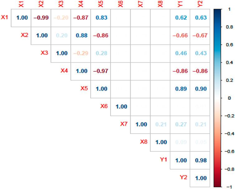
Figure 1. Pearson correlation coefficient matrix of variables.

3.2 Results of classical linear regression model using an application dataset

Here, a multiple linear regression model was fitted with the ordinary least squares (OLS) method for the outcome heating load $\left(Y_1\right)$ regressed with five highly correlated features in the Energy Efficiency Dataset.

Based on the results of the standard OLS regression model, the P value of each regressor is less than $\alpha =5\%$ in Table 1, all the four independent variables or the features: relative compactness $\left(X_1\right)$, surface area $\left(X_2\right)$, wall area $\left(X_3\right)$ and overall height $\left(X_5\right)$ had a significant effect on heating load $\left(Y_1\right)$ except that of roof area $\left(X_4\right)$ that cannot be determined its effect due to its high collinearity with overall height $\left(X_5\right)$. However, the predictor roof area $\left(X_4\right)$ is excluded, computationally hard excluded from the model estimation due to high collinearity with overall height $\left(X_5\right)$ as can be seen in Table 1. The 95% confidence intervals for all feature variables in Table 1 did not overlap zero. Figure 2 shows the significance of all variables and the decision on the null hypothesis, $H_0:{\beta }_{X_j}=0$ for $j=1,2,\dots ,p=5$, for each feature. Thus, the hypothesis is rejected for relative compactness $\left(X_1\right)$ and overall height $\left(X_5\right)$, whereas $H_0$ is accepted for surface area $\left(X_2\right)$ and wall area $\left(X_3\right)$. The estimates of the regression coefficients showed the important negative effect of relative compactness $\left(X_1\right)$ and surface area $\left(X_2\right)$ on heating load $\left(Y_1\right)$. However, the positive effect of wall area $\left(X_3\right)$ and overall height $\left(X_5\right)$ on heating load $\left(Y_1\right)$. In addition to the correlation matrix, the Variance Inflation Factor (VIF) in Table 1 showed the occurrence of high collinearity or Multicollinearity among the features in the dataset. Thus, the standard multiple linear regression with the ordinary least squares (OLS) method reveals biased estimates due to high collinearity among the features. Due to the high Multicollinearity effect in the data, the numerical instability problem in computation occurred in non-deterministic estimates of roof area $\left(X_4\right)$ in the OLS approach (Figure 1; Table 1). This finding is supported by the findings of Ročková and George (2014) and Soofi (1990).

Table 1

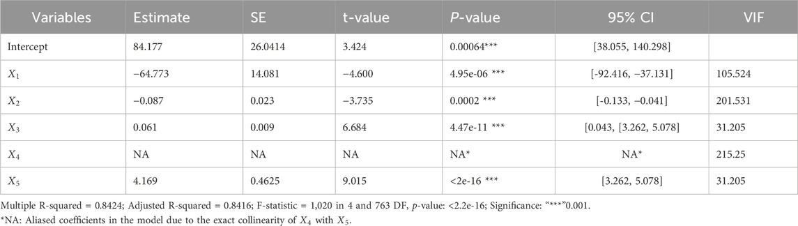
Table 1. Multiple linear regression models using the OLS method for the heating load $\left(Y_1\right)$.

Figure 2

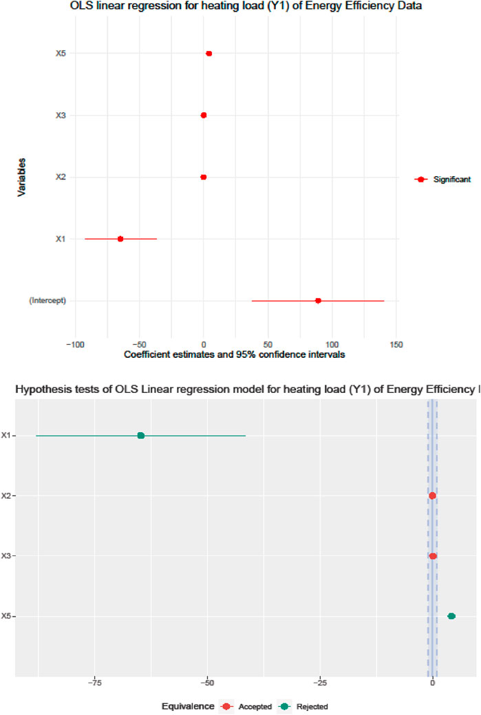
Figure 2. Hypothesis testing of OLS regression estimates and significance.

3.3 Results of Bayesian linear regression models using application data

A Bayesian interpretation of the conventional confidence interval can be understood as the probability (e.g., 95%) that the population parameter lies between the specific upper and lower boundaries ascertained by the posterior distribution in the Bayesian credibility interval (Gelman et al., 2020). By using the same model but different types of prior (weakly informative and shrinkage priors), we test the sensitivity to the prior; and identify the pattern of posterior probabilities and the best-performing model. As per (Van Erp et al., 2018; Depaoli et al., 2020), it is imperative to validate the sensitivity of the prior and likelihood before scrutinizing the influence on the posterior distribution and estimates.

3.4 Model comparison results in applications dataset

Comparing the marginal posterior under various priors is advised since the marginal posterior of regression parameters can be immediately observed when using the Bayesian technique. The Bayesian multiple linear regression with ridge prior (Model 1), Bayesian multiple regression with horseshoe prior (Model 2), Bayesian multiple linear regression with R-square-induced Dirichlet decomposition (R2-D2) prior (Model 3), and Bayesian multiple linear regression with weakly informative prior (Model 4) from the BRMS package in Stan were fitted. To compare the model fit, we compute the Leave-One-Out Information Criteria (LOO-IC), Watanabe-Akaike Information Criteria (WAIC), the Root Mean Squared Error (RMSE), and the Mean Absolute Error (MAE), coefficient of determination $\left(R^2\right)$, and the K-fold criteria of Bayesian-based models fit evaluation criteria and identify the best model after fitting the models.

Based on Table 2, the highest percentage $\left(R^2=84.3\%\right)$ of the total variation in heating load $\left(Y_1\right)$ was explained by the five (5) characteristics of the Bayesian multiple linear regression with weakly informative prior (Bayesian model: 4). Furthermore, the smallest values of LOO-IC, WAIC, K-fold, RMSE, and MAE were observed for Bayesian multiple linear regression with weakly informative prior (Bayesian model: 4). Thus, the Bayesian multiple linear regression model with weakly informative prior (Bayesian Model: 4) is the best-fit model compared to the standard OLS regression, the BRM with ridge prior (Bayesian Model 1), horseshoe prior (Bayesian Model 2) and R-Square-Induced Dirichlet Decomposition (R2-D2) prior (Bayesian Model 3). Sensitivity analysis and inference (estimation, hypothesis testing, and feature selection with prediction) of regression estimates were applied based on the best-fitted BRM (Bayesian Model: 4).

Table 2

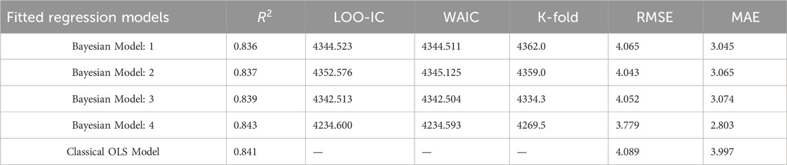
Table 2. Model assessment and comparisons using energy efficiency data.

3.5 Sensitivity analysis in the regression model

Collinearity increases the sensitivity of estimates to the model misspecification. The sensitivity analysis of priors can be evaluated through inference of regression estimates which measures the quantity by which the posterior mean shrinks the OLS estimate of a regression coefficient to zero (Lavine, 1991). Despite its frequent value, sensitivity analysis lacks a technique for validating parameter hypotheses or for calculating Standard Errors (SE) that account for model uncertainty (Taraldsen et al., 2022). Horseshoe prior has been shown to have good theoretical characteristics and performs well in practice, producing outcomes that are quite comparable to those of the spike-and-slab prior (Piironen and Vehtari, 2017b). Therefore, by using sensitivity analysis, posterior inferences are compared under several plausible prior distribution choices (Hamra et al., 2013).

As shown in Table 3, describe the knowledge of the significance of sensitivity analysis and the role of prior distributions when applying Bayesian approaches with a power-scaling sensitivity analysis (using the powerscale_sensitivity function in the R package priorsense). The power-scaling sensitivity analysis indicates prior and likelihood sensitivity for all input feature regression coefficients. Moreover, most of the low likelihood sensitivity was observed for b_X2, $\mathrm{b}\_\mathrm{X}3$, and $\mathrm{b}\_\mathrm{X}4$. This indicates a weak likelihood. However, all show that there is both prior and likelihood sensitivity for two of the fixed effect parameters, b_X1, and $b\_X5$. Moreover, this indicates that there may be a priori data conflict. Power scaling sensitivity analysis on the selected Bayesian model fit shows that there was a longer prior sensitivity and there is appropriate likelihood sensitivity (Table 3; Figure 3).

Table 3

Table 3. BRM Sensitivity Diagnosis with weakly informative prior for the heating load.

Figure 3

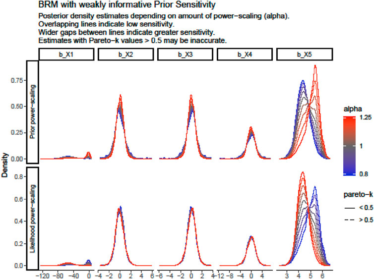
Figure 3. BRMS Sensitivity Analysis Plot of the Posterior Density.

In contrast to a frequentist method, which tests effects against “zero,” Bayesian inference is not predicated on statistical significance. The Bayesian framework provides a probabilistic perspective on the parameters, enabling the evaluation of the associated uncertainty. Therefore, we would argue that the probability of being outside a particular range that can be defined as “practically no effect” (i.e., an insignificant magnitude) is adequate rather than concluding that an effect is present when it merely departs from zero. The Region of Practical Equivalence (ROPE) is the name given to this range. If there are non-independent covariates or occurrences of Multicollinearity among predictors that lead to strong correlations among parameters, the joint parameter distributions may shift within or outside the ROPE. Collinearity disproves ROPE and hypothesis testing based on univariate marginal since the probabilities rely on independence.

The most troubling parameters are those that just partially overlap the ROPE region and the “undecided” parameters’ findings, which could go more in the direction of “rejection” or away from it. For many parameters of the application data set in this manuscript, the undecided decision on the null hypothesis has occurred. Thus, conclusions drawn solely on ROPE are incorrect in the situation of collinearity, since the (joint) distributions of these parameters may experience an increase or reduction in ROPE. (Kruschke, 2014). Another approach for feature importance positions is to check projection predictive variable selection (Piironen and Vehtari, 2015). To check the convergence of MCMC, we draw trace plots and autocorrelation convergence plots with four chins for the best-fitted model. Based on the Bayesian multiple linear regression best-fit model in weakly informative prior for heating load, in Table 4, the credible interval of the intercept and regression coefficients are reported as the frequentist confidence intervals, but the interpretation is from the Bayesian viewpoint. Possible Multicollinearity between b_X5 and b_X1 (r = 0.83) results in inconsistent estimation and biased decisions in the hypothesis tests between frequentist and Bayesian thoughts (Soofi, 1990).

Table 4

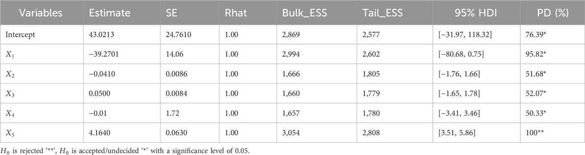
Table 4. Bayesian linear regression best-fitted model in weakly informative prior for heating load $\left(Y_1\right)$.

According to Table 4, based on the data observed, it is believed that there is a 95% probability that heating load $\left(Y_1\right)$ will increase by 35.1% up to 58.6% for each additional 10-cm increase in the overall height $\left(X_5\right)$. Thus, about the data that have been noticed, there is a 95% possibility that the true (unknown) estimate of overall height $\left(X_5\right)$ would be within the interval [3.51, 5.86]. This implies that for every 1-cm increase in the overall height $\left(X_5\right)$, the predicted heating load $\left(Y_1\right)$ increases by 4.64 units. Bayesian regression estimation (Table 4) revealed that the effect of relative compactness $\left(X_1\right)$ on heating load ( ${b\_X}_1$ = −39.27, 95% BCrI [−80.68, 0.75]), such that for each increase of one unit in relative compactness, predicted heating load $\left(Y_1\right)$ decreases by 39.27 units. The effect of surface area $\left(X_2\right)$ on heating load (${b\_X}_2$ = −0.04, 95% BCrI [−1.76, 1.66]), such that for every one-unit increase in surface area $\left(X_2\right)$, the predicted heating load $\left(Y_1\right)$ decreases by 0.04 units. The effect of wall area $\left(X_3\right)$ on heating load (${b\_X}_3$ = 0.05, 95% BCrI [−1.65, 1.78]), such that for each one-unit increase in wall area $\left(X_3\right)$, the predicted heating load $\left(Y_1\right)$ increased by 0.05 units. The effect of roof area $\left(X_4\right)$ on heating load (${b\_X}_4$ =−0.01, 95% BCrI [−3.41, 3.46]), such that for every one-unit increase in roof area $\left(X_4\right)$, the predicted heating load $\left(Y_1\right)$ decreased by 0.01 units. Finally, the intercept has an estimated value of 43.02.

In the Bayesian Regression Model, there should be evidence of checking non-convergence for the four chains before looking at the model summary and valid inferences from the posterior draws. The last three values in Table 4 (“ESS_bulk”, “ESS_tail”, and “Rhat”) provide information on how well the algorithm could estimate the posterior distribution of the parameter. The “Rhat” value is close to or equal to 1, the posterior draws did not have a convergence problem with the MCMC algorithm in Bayesian regression modeling using Stan. In addition, in Figures 4, 5, the four chains mix well for all of the parameters, and therefore there is no evidence of non-convergence. Generally speaking, the posterior mean (called “Estimate”), standard deviation (called “Est. Error”), and two-sided 95% credible intervals (called “l-95% CI” and “u-95% CI”) as HDI are used to summarize each parameter.

Figure 4

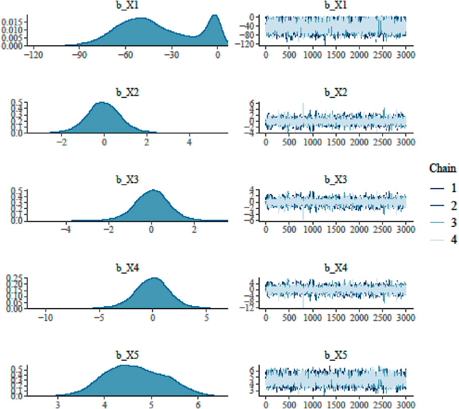
Figure 4. BRMS convergence for the heating load $\left({\mathrm{Y}}_1\right)$ with weakly informative prior.

Figure 5

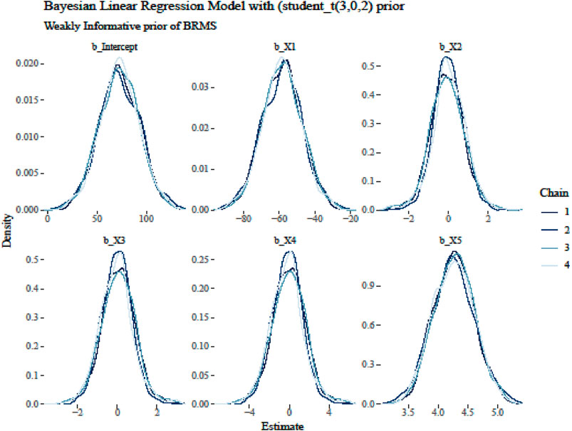
Figure 5. Convergence trace plots of best-fitted Bayesian regression model coefficients.

Interval estimation has a very natural interpretation in Bayesian inference: the 95% CI. The key distinctions between a frequentist CI and a Bayesian HDI or BCrI are assessed here. The results of the classical regression model in Table 1 and Figure 2 showed the significant effect of all input features, the acceptance of four null hypotheses, and the rejection of one hypothesis. The intercept and regression coefficient estimates had huge variations. The proportion of HDIs located within the Region of Practical Equivalence (ROPE) is used as a decision criterion for null hypothesis testing. The HDI plus ROPE decision rule (Test for Practical Equivalence) was suggested by (Kruschke, 2018) to determine if parameter values should be accepted or rejected in light of a null hypothesis that has been expressly stated (Kruschke and Liddell, 2018). As shown in Tables 4, 5; Figures 6–8, the HDI for overall height $\left(X_5\right)$ is completely outside the ROPE [−1.01, 1.01]. The percentage of the posterior enclosed by ROPE [−1.01, 1.01] for overall height $\left(X_5\right)$ is 0%. Therefore, the null hypothesis, $H_0$, for ${b\_X}_5$ is rejected. The Region of Practical Equivalence (ROPE) did not completely cover the HDI for any of the parameters, and none of the hypotheses is accepted. All null hypotheses about the parameters ${b\_X}_1$, ${b\_X}_2$, ${b\_X}_3$, and ${b\_X}_4$ were undecided (Figure 8). It can be used to use the 89% or 95% BCrIs instead of the 95% confidence interval (as in the frequentist framework), as the 89% level provides results which had greater stability (Kruschke, 2014) and reminds us about the uncertainty of such agreements (McElreath, 2018).

Table 5

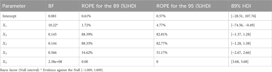
Table 5. Bayes factor and ROPE of the best-fitted model in weakly informative prior.

Figure 6

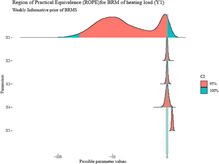
Figure 6. ROPE plot for the best-fitted model parameters.

Figure 7

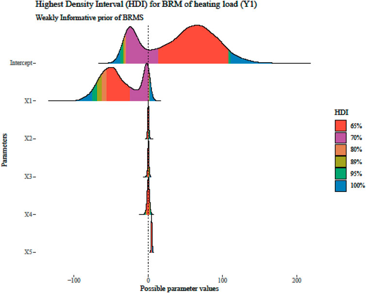
Figure 7. HDI plot for the best-fitted model parameters.

Figure 8

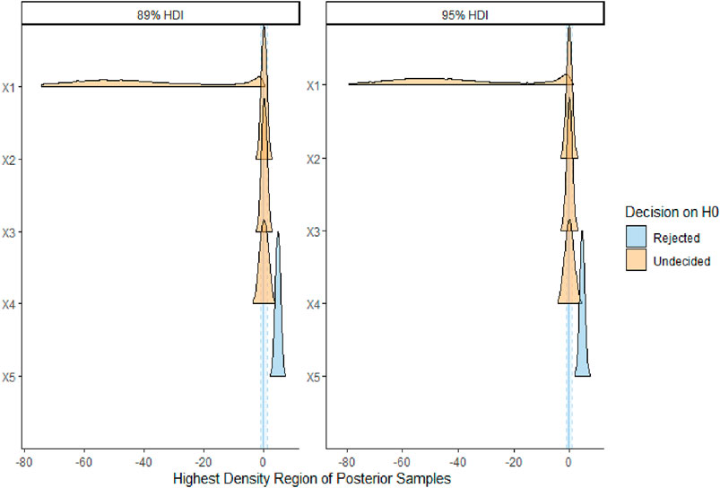
Figure 8. Hypothesis testing in BRM Parameters.

Table 4 also showed that PD and the percentage in ROPE of the linear association between overall height $\left(X_5\right)$ and heating load are about 100% and 0%, respectively, according to certainty and the significant effect of overall height $\left(X_5\right)$ on heating load.

Based on Appendix Table A1, there is only slight fluctuation in the classical and Bayesian estimates of the regression coefficients; however, a huge variation was observed on the intercept, ${\beta }_0$, which has a posterior mean of 43.02 and the classical OLS regression has an intercept as an overall mean of 84.177. The highest posterior density interval is one of the Bayesian Credible Intervals (BCrI) that had threshold values of the posterior distribution that, around the distribution center, represent an interval with the probability of interest (e.g., 95% of the distribution mass). These values are interpreted under the assumption that all values within the interval have higher probabilities of representing the parameter than all values outside them (Hespanhol et al., 2019).

The greatest substitute for the p-value in the frequentist model is the Probability of Direction (PD), which measures the likelihood that the input features’ effects will be positive or negative. Among the independent variables taken as input characteristics, overall height and wall area $\left(X_3\right)$ had a positive effect; whereas other characteristics had negative effects (Figure 9).

Figure 9

Figure 9. Probability of effect direction for the best-fitted model parameters.

In addition to 89% (95%) HDI and ROPE, the Bayes factor is used for decision-making in hypothesis testing. A Bayes factor of more than one is seen as proof against the null hypothesis, and a Bayes factor smaller than 0.33 is interpreted as a considerable indication in favor of the null hypothesis. However, according to (Andraszewicz et al., 2015), a Bayes factor greater than 3 can be considered “substantial” evidence against the null hypothesis.

As shown in Figure 10, the posterior predictive distribution that compares the observed data $\left(y\right)$ with the posterior predicted values $\left(y_{rep}\right)$ had a slightly identical pattern and the estimate of the kernel density for the data and the posterior predictive values are comparable. Based on the variables in Figure 11 and the selection of the posterior predicted variables projected posterior predictive variable selection determined with the cv_varsel function by computing a LOO-CV estimation of the most accurate prediction performance for the best model with a certain number of variables, the five input features or independent variables are important for estimating the heating load. Furthermore, the ranking of the significance of variables for heating load is overall height $\left(X_5\right)$, wall area $\left(X_3\right)$, relative compactness $\left(X_1\right)$, surface area $\left(X_2\right),$ and roof area $\left(X_4\right)$. Cross -Validation (CV) ranking using the projection predictive variable selection technique in Stan was applied to determine the position of each independent variable in sub-model size from full data as shown in Figure 11. In the OLS approach, the non-deterministic independent variable, roof area X4, became the least important in the Bayesian methods (Piironen and Vehtari, 2015).

Figure 10

Figure 10. BRMS posterior predictive check for heating load $\left(Y_1\right)$.

Figure 11

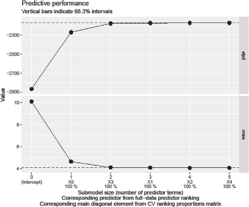
Figure 11. Variable Selection for Predictive Performance of Heating Load $\left(Y_1\right)$.

4 Conclusion and recommendation

This manuscript demonstrates the effect of Multicollinearity in estimation and hypothesis tests of linear regression models with OLS and Bayesian approaches of several prior distributions using collinear energy efficiency data. Preliminarily strongly correlated independent variables or features with the outcome or dependent variables were selected based on the correlation analysis. The correlation analysis and the VIF results showed the occurrence of high Multicollinearity among predictors in the data. The excluded variable (roof area $\left.\left(X_4\right)\right)$ in the OLS model due to collinearity has been estimated using the Bayesian approach. Four different Bayesian multiple regression models were fitted with identical five input variables with four different prior information. Among the classical OLS regression model, the four fitted Bayesian models: Bayesian Multiple Regression (BMR) with ridge prior (Model 1), BMR with horseshoe prior (Model 2), BMR with R-square-induced Dirichlet Decomposition (R2-D2) prior (Model 3), and BMR with weakly informative prior (Model 4), the Bayesian Multiple Regression (BMR) model with weakly informative prior was best fitted. The classical regression result showed that all five independent variables have a significant effect on the heating load. However, the hypothesis indicates acceptance of the first four null hypotheses. The posterior mean estimates and Standard Error (SE) of every coefficient are different from the equivalent frequentist OLS estimates and SE. There is an effect for regression parameter inference (estimation, hypothesis testing, and prediction) due to Multicollinearity among the input features. The Bayesian hypothesis testing using HDI plus ROPE showed a rejection of a null hypothesis for the overall height and an undecided decision on the other parameters due to the non-independence of predictors. However, the importance ranking of input features was checked by the selection of projection predictive variables showing overall height, wall area, relative compactness, surface area, and roof area. It is necessary to check the Multicollinearity effect for regression modeling with the Bayesian and frequentist approaches for any applied research in science, engineering, agriculture, health, and other discipline datasets. In addition, by careful identification of the key drivers of energy efficiency in buildings, this study provides a valuable framework for researchers, policymakers, and industry stakeholders to implement cleaner and more sustainable energy estimation practices.

This study considered a full model with overall samples or train subsets and assessed the difference in posterior estimates under the OLS approach and four distinct priors. However, fitting several sub-models with sub-samples as split subsets of the overall dataset and using another test of posterior difference such as the Kolmogorov–Smirnov test was not used. It is suggested to use K-fold cross-validation, ensemble, data augmentation, and data simplification techniques by split subsets act as the testing set, and the remaining folds will train the model.

Further research could concentrate on Bayes factors that assess the significance of correlated covariates jointly are more appropriate, and certain priors may be more negatively affected in such a setting. This is in addition to the routine examination of the correlation matrix and the posterior distribution in various prior settings.

Data availability statement

The original contributions presented in the study are included in the article/Supplementary material, further inquiries can be directed to the corresponding author.

Author contributions

LA-E: Conceptualization, Investigation, Methodology, Project administration, Resources, Software, Visualization, Writing–original draft, Writing–review and editing. EE: Conceptualization, Data curation, Formal Analysis, Methodology, Resources, Software, Validation, Writing–original draft, Writing–review and editing. YM: Conceptualization, Data curation, Resources, Supervision, Validation, Visualization, Writing–original draft, Writing–review and editing.

Funding

The author(s) declare that financial support was received for the research, authorship, and/or publication of this article. This is supported by Princess Nourah bint Abdulrahman University Researchers Supporting Project number (PNURSP2024R443), Princess Nourah bint Abdulrahman University, Riyadh, Saudi Arabia.

Acknowledgments

Princess Nourah bint Abdulrahman University Researchers Supporting Project number (PNURSP2024R443), Princess Nourah bint Abdulrahman University, Riyadh, Saudi Arabia.

Conflict of interest

The authors declare that the research was conducted in the absence of any commercial or financial relationships that could be construed as a potential conflict of interest.

Publisher’s note

All claims expressed in this article are solely those of the authors and do not necessarily represent those of their affiliated organizations, or those of the publisher, the editors and the reviewers. Any product that may be evaluated in this article, or claim that may be made by its manufacturer, is not guaranteed or endorsed by the publisher.

Abbreviations

BCrI, Bayesian Credible Interval; BF, Bayes factor; BMR, Bayesian multiple regression; BRMS, Bayesian regression model using stan; CI, Confidence interval; ELPD, Expected log-posterior predictive density; ESS, Effective sample size; HDI, Highest density interval; LOO-IC, Leave-one-out information criteria; MAE, Mean absolute error; MCMC, Markov chain monte carlo; OLS, Ordinary least squares; PD, Probability of direction; R2, Coefficient of determination; R2-D2, R-Square induced dirichlet decomposition; Rhat, Scale reduction factor; RMSE, Root mean squared error; ROPE, Region of practical equivalence; VIF, Variance inflation factor; WAIC, Watanabe-Akaike information criteria.

References

Abdou, N., El Mghouchi, Y., Jraida, K., Hamdaoui, S., Hajou, A., and Mouqallid, M. (2022). Prediction and optimization of heating and cooling loads for low energy buildings in Morocco: an application of hybrid machine learning methods. J. Build. Eng. 61, 105332. doi:10.1016/J.JOBE.2022.105332

CrossRef Full Text | Google Scholar

Ackermann, R. (2019). “Bayesian statistical inference,” in Nondeductive Inference. (London: Routledge), 83–103. doi:10.4324/9780367853907-5

CrossRef Full Text | Google Scholar

Ahmadi, M. (2024). Building energy efficiency: using machine learning algorithms to accurately predict heating load. Asian J. Civ. Eng. 25 (4), 3129–3139. doi:10.1007/s42107-023-00967-w

CrossRef Full Text | Google Scholar

Alin, A. (2010). Multicollinearity. Wiley Interdiscip. Rev. Comput. Stat. 2 (3), 370–374. doi:10.1002/WICS.84

CrossRef Full Text | Google Scholar

Andraszewicz, S., Scheibehenne, B., Rieskamp, J., Grasman, R., Verhagen, J., and Wagenmakers, E. J. (2015). An introduction to Bayesian hypothesis testing for management research. J. Manag. 41 (2), 521–543. doi:10.1177/0149206314560412

CrossRef Full Text | Google Scholar

Assaf, A. G., and Tsionas, M. (2021a). A Bayesian solution to multicollinearity through unobserved common factors. Tour. Manag. 84, 104277. doi:10.1016/J.TOURMAN.2020.104277

CrossRef Full Text | Google Scholar

Assaf, A. G., and Tsionas, M. (2021b). Testing for collinearity using Bayesian Analysis, J. Hosp. Tour. Res., 45(6), 1131–1141. doi:10.1177/1096348021990841

CrossRef Full Text | Google Scholar

Baranova, D., Sovetnikov, D., Semashkina, D., and Borodinecs, A. (2017). Correlation of energy efficiency and thermal comfort depending on the ventilation strategy. Procedia Eng. 205, 503–510. doi:10.1016/J.PROENG.2017.10.403

CrossRef Full Text | Google Scholar

Bui, D. T., Moayedi, H., Anastasios, D., and Foong, L. K. (2019). Predicting heating and cooling loads in energy-efficient buildings using two hybrid intelligent models. Appl. Sci. 9 (17), 3543. doi:10.3390/APP9173543

CrossRef Full Text | Google Scholar

Bürkner, P. C. (2017). brms: an R package for Bayesian multilevel models using Stan. J. Stat. Softw. 80 (1), 1–28. doi:10.18637/jss.v080.i01

CrossRef Full Text | Google Scholar

Chicco, D., Warrens, M. J., and Jurman, G. (2021). The coefficient of determination R-squared is more informative than SMAPE, MAE, MAPE, MSE and RMSE in regression analysis evaluation. PeerJ Comput. Sci. 7, e623. doi:10.7717/PEERJ-CS.623

PubMed Abstract | CrossRef Full Text | Google Scholar

Çolak, A. B., Sindhu, T. N., Lone, S. A., Shafiq, A., and Abushal, T. A. (2023). Reliability study of generalized Rayleigh distribution based on inverse power law using artificial neural network with Bayesian regularization. Tribol. Int. 185, 108544. doi:10.1016/J.TRIBOINT.2023.108544

CrossRef Full Text | Google Scholar

Consonni, G., Fouskakis, D., Liseo, B., and Ntzoufras, I. (2018). Prior distributions for objective Bayesian analysis. Bayesian Anal. 13 (2), 627–679. doi:10.1214/18-BA1103

CrossRef Full Text | Google Scholar

Depaoli, S., Winter, S. D., and Visser, M. (2020). The importance of prior sensitivity analysis in Bayesian statistics: demonstrations using an interactive Shiny App. Front. Psychol. 11, 608045. doi:10.3389/fpsyg.2020.608045

PubMed Abstract | CrossRef Full Text | Google Scholar

Farrar, D. E., and Glauber, R. R. (1967). Multicollinearity in regression analysis: the problem revisited. Rev. Econ. Statistics 49 (1), 92. doi:10.2307/1937887

CrossRef Full Text | Google Scholar

Felipe, V. P. S., Silva, M. A., Valente, B. D., and Rosa, G. J. M. (2015). Using multiple regression, Bayesian networks and artificial neural networks for prediction of total egg production in European quails based on earlier expressed phenotypes. Poult. Sci. 94 (4), 772–780. doi:10.3382/PS/PEV031

PubMed Abstract | CrossRef Full Text | Google Scholar

Frost, J. (2019). Multicollinearity in regression analysis: problem, detection, and solutions. Statisticsbyjim.Com. Available at: https://statisticsbyjim.com/regression/multicollinearity-in-regression-analysis/%0Ahttps://statisticsbyjim.com/regression/multicollinearity-in-regression-analysis/%0Ahttps://statisticsbyjim.com/regression/multicollinearity-in-regression-analysis/%0Ahttp:/.

Google Scholar

Garg, R. (1984). Ridge regression in the presence of multicollinearity. Psychol. Rep. 54 (2), 559–566. doi:10.2466/pr0.1984.54.2.559

CrossRef Full Text | Google Scholar

Gebrie, Y. F. (2021). Bayesian regression model with application to a study of food insecurity in household level: a cross sectional study. BMC Public Health 21 (1), 619. doi:10.1186/s12889-021-10674-3

PubMed Abstract | CrossRef Full Text | Google Scholar

Gelman, A., Carlin, J. B., Stern, H. S., Dunson, D. B., Vehtari, A., and Rubin, D. B. (2013). Bayesian data analysis, third edition. 3rd Edn. (Florida: CRC Press).

Google Scholar

Gelman, A., Vehtari, A., Simpson, D., Margossian, C. C., Carpenter, B., Yao, Y., et al. (2020). Bayesian workflow. Available at: http://arxiv.org/abs/2011.01808.

Google Scholar

Grzenda, W. (2016). Informative versus non-informative prior distributions and their impact on the accuracy of Bayesian inference. Statistics in Transition new series 17 (4), 763–780. doi:10.59170/stattrans-2016-042

CrossRef Full Text | Google Scholar

Guo, J., Yun, S., Meng, Y., He, N., Ye, D., Zhao, Z., et al. (2023). Prediction of heating and cooling loads based on light gradient boosting machine algorithms. Build. Environ. 236, 110252. doi:10.1016/J.BUILDENV.2023.110252

CrossRef Full Text | Google Scholar

Hamra, G. B., MacLehose, R. F., and Cole, S. R. (2013). Sensitivity analyses for sparse-data problems—using weakly informative Bayesian priors. Epidemiol. (Cambridge, Mass.) 24 (2), 233–239. doi:10.1097/EDE.0B013E318280DB1D

PubMed Abstract | CrossRef Full Text | Google Scholar

Hespanhol, L., Vallio, C. S., Costa, L. M., and Saragiotto, B. T. (2019). Understanding and interpreting confidence and credible intervals around effect estimates. Braz. J. Phys. Ther. 23 (4), 290–301. doi:10.1016/J.BJPT.2018.12.006

PubMed Abstract | CrossRef Full Text | Google Scholar

Jammulamadaka, H. S., Gopalakrishnan, B., Chaudhari, S., Sundaramoorthy, S., Mehta, A. R., and Mostafa, R. (2022). Evaluation of energy efficiency performance of heated windows. Energy Eng. J. Assoc. Energy Eng. 119 (1), 1–16. doi:10.32604/EE.2022.017363

CrossRef Full Text | Google Scholar

Jaya, I. G. N. M., Tantular, B., and Andriyana, Y. (2019). A Bayesian approach on multicollinearity problem with an Informative Prior. J. Phys. Conf. Ser. 1265 (1), 012021. doi:10.1088/1742-6596/1265/1/012021

CrossRef Full Text | Google Scholar

Jitkongchuen, D., and Pacharawongsakda, E. (2019). “Prediction heating and cooling loads of building using evolutionary grey Wolf algorithms,” in 2019 - 4th International Conference on Digital Arts, Media and Technology and 2nd ECTI Northern Section Conference on Electrical, Electronics, Computer and Telecommunications Engineering (ECTI DAMT-NCON), Nan, Thailand, 30 January 2019–02 February 2019, 93–97. doi:10.1109/ECTI-NCON.2019.8692232

CrossRef Full Text | Google Scholar

Kaczmarczyk, M. (2024). Building energy characteristic evaluation in terms of energy efficiency and ecology. Energy Convers. Manag. 306, 118284. doi:10.1016/J.ENCONMAN.2024.118284

CrossRef Full Text | Google Scholar

Kallioinen, N., Paananen, T., Bürkner, P. C., and Vehtari, A. (2024). Detecting and diagnosing prior and likelihood sensitivity with power-scaling. Statistics Comput. 34 (1), 57. doi:10.1007/s11222-023-10366-5

CrossRef Full Text | Google Scholar

Kavaklioglu, K. (2018). Robust modeling of heating and cooling loads using partial least squares towards efficient residential building design. J. Build. Eng. 18, 467–475. doi:10.1016/J.JOBE.2018.04.018

CrossRef Full Text | Google Scholar

Kim, D. D., and Suh, H. S. (2021). Heating and cooling energy consumption prediction model for high-rise apartment buildings considering design parameters. Energy Sustain. Dev. 61, 1–14. doi:10.1016/J.ESD.2021.01.001

CrossRef Full Text | Google Scholar

Kim, J. H. (2019). Multicollinearity and misleading statistical results. Korean J. Anesthesiol. 72 (6), 558–569. doi:10.4097/KJA.19087

PubMed Abstract | CrossRef Full Text | Google Scholar

Kim, S.-H., Cohen, A. S., Kwak, M., and Lee, J. (2019). Priors in Bayesian estimation under the Rasch model. J. Appl. Meas. 20 (4), 384–398. Available at: http://www.ncbi.nlm.nih.gov/pubmed/31730545.

PubMed Abstract | Google Scholar

Kruschke, J. K. (2014). “Doing Bayesian data analysis: a tutorial with R, JAGS, and Stan, second edition,” in Doing bayesian data analysis: a tutorial with R, JAGS, and stan. 2nd ed. (Indiana, United States: Indiana University in Bloomington). doi:10.1016/B978-0-12-405888-0.09999-2

CrossRef Full Text | Google Scholar

Kruschke, J. K. (2018). Rejecting or accepting parameter values in Bayesian estimation. Adv. Methods Pract. Psychol. Sci. 1 (2), 270–280. doi:10.1177/2515245918771304

CrossRef Full Text | Google Scholar

Kruschke, J. K., and Liddell, T. M. (2018). The Bayesian new statistics: hypothesis testing, estimation, meta-analysis, and power analysis from a Bayesian perspective. Psychonomic Bull. Rev. 25 (1), 178–206. doi:10.3758/s13423-016-1221-4

PubMed Abstract | CrossRef Full Text | Google Scholar

Lavine, M. (1991). Sensitivity in Bayesian statistics: the prior and the likelihood. J. Am. Stat. Assoc. 86 (414), 396. doi:10.2307/2290583

CrossRef Full Text | Google Scholar

Leamer, E. E. (1973). Multicollinearity: a Bayesian interpretation. Rev. Econ. Statistics; JSTOR 55, 371. doi:10.2307/1927962

CrossRef Full Text | Google Scholar

Lemoine, N. P. (2019). Moving beyond noninformative priors: why and how to choose moving beyond noninformative priors: why and how to choose weakly informative priors in Bayesian analyses weakly informative priors in Bayesian analyses. Available at: https://epublications.marquette.edu/bio_fac.

Google Scholar

Mahajan, V., Jain, A. K., and Bergier, M. (1977). Parameter estimation in marketing models in the presence of multicollinearity: an application of ridge regression. J. Mark. Res. 14 (4), 586–591. doi:10.1177/002224377701400419

CrossRef Full Text | Google Scholar

McElreath, R. (2018). “Statistical rethinking: a bayesian course with examples in R and stan,” in Statistical rethinking: a bayesian course with examples in R and stan. 2nd ed. (Germany: Leipzig University), 2011. doi:10.1201/9781315372495

CrossRef Full Text | Google Scholar

Mettle, F., Asiedu, L., Quaye, E., and Asare-Kumi, A. (2016). Comparison of least squares method and bayesian with multivariate normal prior in estimating multiple regression parameters. Br. J. Math. Comput. Sci. 15 (1), 1–8. doi:10.9734/bjmcs/2016/23145

CrossRef Full Text | Google Scholar

Miroshnikov, A., Savel’ev, E., and Conlon, E. M. (2015). BayesSummaryStatLM: an R package for bayesian linear models for big data and data science. Available at: http://arxiv.org/abs/1503.00635.

Google Scholar

Moletsane, P. P., Motlhamme, T. J., Malekian, R., and Bogatmoska, D. C. (2018). “Linear regression analysis of energy consumption data for smart homes,” in 2018 41st International Convention on Information and Communication Technology, Electronics and Microelectronics, MIPRO 2018 - Proceedings, Opatija, Croatia, 21-25 May 2018, 395–399. doi:10.23919/MIPRO.2018.8400075

CrossRef Full Text | Google Scholar

Müller, U. K. (2012). Measuring prior sensitivity and prior informativeness in large Bayesian models. J. Monetary Econ. 59 (6), 581–597. doi:10.1016/j.jmoneco.2012.09.003

CrossRef Full Text | Google Scholar

Mummolo, J., and Peterson, E. (2018). Improving the interpretation of fixed effects regression results. Political Sci. Res. Methods 6 (4), 829–835. doi:10.1017/psrm.2017.44

CrossRef Full Text | Google Scholar

Nasional, K., Matematika, P., Pembelajarannya, D., Jaya, N. M., Tantular, B., and Andriyana, Y. (2019). A Bayesian approach on multicollinearity problem with an Informative Prior. J. Phys. Conf. Ser. 1265 (1), 012021. doi:10.1088/1742-6596/1265/1/012021

CrossRef Full Text | Google Scholar

Neubauer, A., Brandt, S., and Kriegel, M. (2024). Relationship between feature importance and building characteristics for heating load predictions. Appl. Energy 359, 122668. doi:10.1016/J.APENERGY.2024.122668

CrossRef Full Text | Google Scholar

Nithin, N. (2023). Bayesian statistics: understanding the principles and applications of Bayesian inference. Res. Rev. J. Statistics Math. Sci. 9(1), 18–19. doi:10.4172/JStatsMathSci.9.1.009

CrossRef Full Text | Google Scholar

Oluwadare, O. O. (2021). Sensitivity of priors in the presence of collinearity in vector autoregressive model: a Monte Carlo study. Thailand Statistician. Available at: https://ph02.tci-thaijo.org/index.php/thaistat/article/view/243857/165412.

Google Scholar

Pesaran, M. H., and Smith, R. P. (2019). A Bayesian analysis of linear regression models with highly collinear regressors. Econ. Statistics 11, 1–21. doi:10.1016/J.ECOSTA.2018.10.001

CrossRef Full Text | Google Scholar

Piironen, J., and Vehtari, A. (2015). Projection predictive variable selection using Stan+R. Available at: http://arxiv.org/abs/1508.02502.

Google Scholar

Piironen, J., and Vehtari, A. (2017a). “On the hyperprior choice for the global shrinkage parameter in the horseshoe prior,” in Proceedings of the 20th International Conference on Artificial Intelligence and Statistics, AISTATS 2017, 20–22 April 2017, Fort Lauderdale, FL, USA, doi:10.48550/arxiv.1610.05559

CrossRef Full Text | Google Scholar

Piironen, J., and Vehtari, A. (2017b). Sparsity information and regularization in the horseshoe and other shrinkage priors. Electron. J. Statistics 11 (2), 5018–5051. doi:10.1214/17-EJS1337SI

CrossRef Full Text | Google Scholar

Polson, N. G., and Scott, J. G. (2010). Shrink globally, act locally: sparse Bayesian regularization and prediction. Bayesian Statistics 9, 501–538.

Google Scholar

Reim, M., Körner, W., Chhugani, B., and Weismann, S. (2017). Correlation between energy efficiency in buildings and comfort of the users. Energy Procedia 122, 457–462. doi:10.1016/J.EGYPRO.2017.07.291

CrossRef Full Text | Google Scholar

Ročková, V., and George, E. I. (2014). Negotiating multicollinearity with spike-and-slab priors. Metron 72 (2), 217–229. doi:10.1007/s40300-014-0047-y

PubMed Abstract | CrossRef Full Text | Google Scholar

Samira, M. S. (2023). Comparison between multiple regression and bayesian regression with application. Inf. Statistics 4 (1), 88–100.

Google Scholar

Sekhar Roy, S., Roy, R., and Balas, V. E. (2018). Estimating heating load in buildings using multivariate adaptive regression splines, extreme learning machine, a hybrid model of MARS and ELM. Renew. Sustain. Energy Rev. 82, 4256–4268. doi:10.1016/J.RSER.2017.05.249

CrossRef Full Text | Google Scholar

Seltzer, M. H. (1993). Sensitivity analysis for fixed effects in the hierarchical model: a Gibbs sampling approach. J. Educ. Statistics 18 (3), 207–235. doi:10.3102/10769986018003207

CrossRef Full Text | Google Scholar

Shrestha, N. (2020). Detecting multicollinearity in regression analysis. Am. J. Appl. Math. Statistics 8 (2), 39–42. doi:10.12691/AJAMS-8-2-1

CrossRef Full Text | Google Scholar

Sinay, M. S., and Hsu, J. S. J. (2014). Bayesian inference of a multivariate regression model. J. Probab. Statistics 2014, 1–13. doi:10.1155/2014/673657

CrossRef Full Text | Google Scholar

Sindhu, T. N., Çolak, A. B., Lone, S. A., and Shafiq, A. (2023). Reliability study of generalized exponential distribution based on inverse power law using artificial neural network with Bayesian regularization. Qual. Reliab. Eng. Int. 39 (6), 2398–2421. doi:10.1002/QRE.3352

CrossRef Full Text | Google Scholar

Soofi, E. S. (1990). Effects of collinearity on information about regression coefficients. J. Econ. 43 (3), 255–274. doi:10.1016/0304-4076(90)90120-I

CrossRef Full Text | Google Scholar

Tahmasebinia, F., He, R., Chen, J., Wang, S., and Sepasgozar, S. M. E. (2023). Building energy performance modeling through regression analysis: a case of tyree energy technologies building at UNSW Sydney. Buildings 13 (4), 1089. doi:10.3390/BUILDINGS13041089

CrossRef Full Text | Google Scholar

Tanoe, V., Henderson, S., Shahirinia, A., and Bina, M. T. (2021). Bayesian and non-Bayesian regression analysis applied on wind speed data. J. Renew. Sustain. Energy 13 (5), 53303. doi:10.1063/5.0056237

CrossRef Full Text | Google Scholar

Taraldsen, G., Tufto, J., and Lindqvist, B. H. (2022). Improper priors and improper posteriors. Scand. J. Statistics 49 (3), 969–991. doi:10.1111/SJOS.12550

CrossRef Full Text | Google Scholar

Taskin, D., Dogan, E., and Madaleno, M. (2022). Analyzing the relationship between energy efficiency and environmental and financial variables: a way towards sustainable development. Energy 252, 124045. doi:10.1016/J.ENERGY.2022.124045

CrossRef Full Text | Google Scholar

Tsanas, A., and Xifara, A. (2012). Energy efficiency. UCI machine learning repository. doi:10.24432/C51307

CrossRef Full Text | Google Scholar

Ullah, M. I. (2021). Multicollinearity in linear regression models. Itfeature.Com. Available at: https://itfeature.com/correlation-and-regression-analysis/multicollinearity-in-linear-regression-models.

Google Scholar

van de Schoot, R., and Depaoli, S. (2014). Bayesian statistics: where to start and what to report. Eur. Health Psychol. 16 (2), 74–84.

Google Scholar

van Erp, S., Mulder, J., and Oberski, D. L. (2018). Prior sensitivity analysis in default Bayesian structural equation modeling. Psychol. Methods 23 (2), 363–388. doi:10.1037/met0000162

PubMed Abstract | CrossRef Full Text | Google Scholar

Vehtari, A., Gelman, A., and Gabry, J. (2017). Practical Bayesian model evaluation using leave-one-out cross-validation and WAIC. Statistics Comput. 27 (5), 1413–1432. doi:10.1007/s11222-016-9696-4

CrossRef Full Text | Google Scholar

Vijayaragunathan, R., John, K. K., and Srinivasan, M. R. (2023). Identifying the influencing factors for the BMI by bayesian and frequentist multiple linear regression models: a comparative study. Indian J. Community Med. 48 (5), 659–665. doi:10.4103/IJCM.IJCM_119_22

PubMed Abstract | CrossRef Full Text | Google Scholar

Voss, D. S. (2004). Multicollinearity. Encyclopedia of social measurement, three-volume set, 2, V2-759-V2-770. doi:10.1016/B0-12-369398-5/00428-X

CrossRef Full Text | Google Scholar

Willis, C. E., and Perlack, R. D. (1978). Multicollinearity: effects, symptoms, and remedies. J. Northeast. Agric. Econ. Counc. 7 (1), 55–61. doi:10.1017/S0163548400001989

CrossRef Full Text | Google Scholar

Wu, T., Narisetty, N. N., and Yang, Y. (2023). Statistical inference via conditional Bayesian posteriors in high-dimensional linear regression. Electron. J. Stat. 17 (1), 769–797. doi:10.1214/23-EJS2113

CrossRef Full Text | Google Scholar

Youssef, A. M. A. E. R. (2022). Detecting of multicollinearity, autocorrelation and heteroscedasticity in regression analysis. Advances 3 (3), 140–152. doi:10.11648/J.ADVANCES.20220303.24

CrossRef Full Text | Google Scholar

Zhang, Y. D., Naughton, B. P., Bondell, H. D., and Reich, B. J. (2022). Bayesian regression using a prior on the model fit: the R2-D2 shrinkage prior. J. Am. Stat. Assoc. 117 (538), 862–874. doi:10.1080/01621459.2020.1825449

CrossRef Full Text | Google Scholar

Zianis, D., Spyroglou, G., Tiakas, E., and Radoglou, K. M. (2016). Bayesian and classical models to predict aboveground tree biomass allometry. For. Sci. 62 (3), 247–259. doi:10.5849/FORSCI.15-045

CrossRef Full Text | Google Scholar

Appendix

TABLE A1

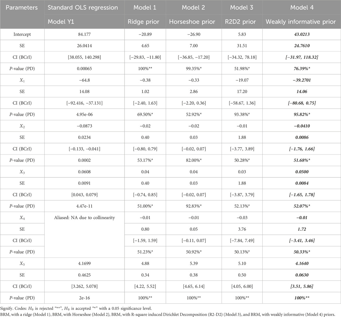
TABLE A1. Sensitivity analysis of fitted models estimates for Energy Efficiency data.