 Chao Xing
 Xinze Xi
- Electric Power Research Institute of Yunnan Power Grid Co., Ltd., Kunming, China
The role of load modeling in power systems is crucial for both operational and regulatory considerations. It is essential to develop an effective and reliable method for optimizing load modeling parameter identification. In this paper, the dung beetle algorithm is improved by using the good point set, and a load model parameter identification strategy based on the good point set dung beetle optimization algorithm (GDBO) within the framework of the measurement-based load modeling method. The proposed parameter identification strategy involves utilizing PMU voltage data as input, selecting a comprehensive load model, and refining the initialization process based on the good point set to mitigate the influence of local maxima. Through iterative optimization of the objective function using the Dung Beetle Optimizer (DBO) algorithm, the optimal parameters for the comprehensive load model are determined, enhancing the model’s ability to accurately capture the power curve. Analysis of examples pertaining to PMU-measured modeling parameter identification reveals that the proposed GDBO algorithm, which incorporates a good point set, outperforms alternative methods such as the improved differential evolution algorithm (IDE), particle swarm optimization algorithm (PSO), grey wolf optimization algorithm (GWO), and conventional DBO algorithm. This demonstrates the superior performance of the introduced approach in the context of load model parameter identification.
1 Introduction
At present, digital simulation plays an irreplaceable role in power systems across various domains such as power network planning, operation, control, and personnel training (Zhang et al., 2020; Yang et al., 2022a; Diao et al., 2023; Wu et al., 2023; Zhang et al., 2023a; Zhu et al., 2023). The accuracy of the simulation results depends on the conformity of the adopted component models and parameters. Selecting an inappropriate load model in power system simulation can lead to deviations in the simulation results from the actual situation, potentially resulting in misallocation of planning funds and operational decision-making errors (Ju, 2015; Xu et al., 2023). Therefore, in the process of dynamic simulation, it is very important to select a suitable load model to describe the load of a specific area (Swarupa et al., 2024).
Load modeling has two main approaches (Wang et al., 2014; Chen et al., 2020; Yang et al., 2022b) in power systems: component-based and measurement-based. The component-based load modeling first needs to count the characteristics of various typical loads, the proportion of load equipment, and the composition of loads (Wu et al., 2022; Fu et al., 2023; Yang et al., 2024), then derive the mathematical models and parameters of various typical loads, and finally integrate the statistical data to establish the model of load nodes. However, the load composition will change with time, the statistical workload is large, and the voltage characteristics of reactive power cannot be accurately obtained, so there are few practical applications. In contrast, measurement-based load modeling considers the power system as a stochastic system, first determines the model structure, then identifies the model parameters based on the measured data, and verifies its generalization ability (Wang et al., 2019; Zhang et al., 2023b; Zhou et al., 2023). This method requires the installation of a load characteristic recording device at the load node, which usually obtains data for identification under large disturbances. Although there are some drawbacks to measurement-based load modeling, it can be widely used in practice by using input-output models to solve the problem of complex load components without much statistical work (Zhang, 2007; Yang et al., 2018).
With the continuous development and popularization of artificial intelligence, intelligent algorithms have been widely used in the research of load modeling technology (Wang et al., 2011; Wang et al., 2020; Kang et al., 2021; Guo et al., 2022). Reference (Wang et al., 2020; Guo et al., 2022) has applied the grey wolf optimization (GWO) algorithm to load modeling based on its advantages of better global convergence, fewer adjustment parameters, and easy identification. It has been proven that the GWO algorithm can improve the accuracy of load modeling. Reference (Kang et al., 2021) adds the weight of flight inertia, global optimum, and flight interference factor to the butterfly algorithm to avoid the butterfly algorithm falling into the local optimum prematurely and improve the accuracy of the comprehensive load model. In order to prevent local convergence of the algorithm and increase the accuracy of identification findings, the chaos algorithm is incorporated into the ant colony method in Reference (Wang et al., 2011). However, due to the mixing of algorithms, the selection of parameters becomes complicated.
The dung beetle optimization (DBO) algorithm is an intelligent optimization algorithm that achieves global exploration and local development through the ball rolling, oviposition, foraging and stealing behavior of dung beetles (Yang et al., 2022c; Xue and Shen, 2022). The algorithm has the ability for global exploration and local development, which can speed up convergence and prevent premature phenomena. Presently, it has found extensive application in diverse research domains, including but not limited to range-free localization (Pan and Bu, 2023) and neural network training (Li et al., 2023). However, few scholars have applied the DBO algorithm to the research of load modeling.
In summary, this study employs the Dung Beetle Optimizer (DBO) algorithm, alternatively recognized as the Good Point Set Dung Beetle Optimizer (GDBO), to ascertain and refine the essential parameters inherent in the comprehensive load model. The PMU measured data is used as the input samples for load modeling. The optimal parameters of the load model are achieved through repeated optimization of the objective function, improving the model’s fit to the power curve. Finally, a comparison between the optimized sample curves and model responses produced by the proposed algorithm and the algorithms for improved differential evolution (IDE) (Xu et al., 2009a; Pattanaik et al., 2017), particle swarm optimization (PSO) (Fang et al., 2022), GWO (Wang et al., 2020; Guo et al., 2022), and DBO is made. This confirms that the proposed method is more accurate and solves load modeling parameters more quickly.
The paper is organized as follows: The establishment of the comprehensive load model is shown in the second chapter. The third chapter introduces the parameter identification of the integrated load model, including the principle of parameter identification, parameter identification method, the improvement of the identification method and the specific process of the identification algorithm. In the fourth chapter, the example simulation of parameter identification is carried out. The fifth chapter gives the conclusion.
2 Comprehensive load model
The comprehensive load model comprises a static ZIP load model and a three-order induction motor model in parallel (Liu, 2007; Sheng et al., 2021; Yang et al., 2022d; Wang et al., 2023). The model is shown in the following Figure 1.
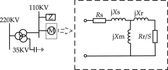
Figure 1. Equivalent structure of integrated load model.
The static ZIP part adopts a polynomial model, which can be described as follows Equation 1:
in the above formula, we use
The induction motor part can be described as Equations 2, 3:
In the formula:
where:
To sum up, the parameters to be identified are
3 Parameter identification of load model
3.1 Principle of parameter identification
After determining the model structure, it is necessary to select an efficient and reliable optimization algorithm for parameter identification. At the core of parameter identification lies the estimation of model parameters by fitting a mathematical model of the system using input and output data. The principles of this process are illustrated in Figure 2.
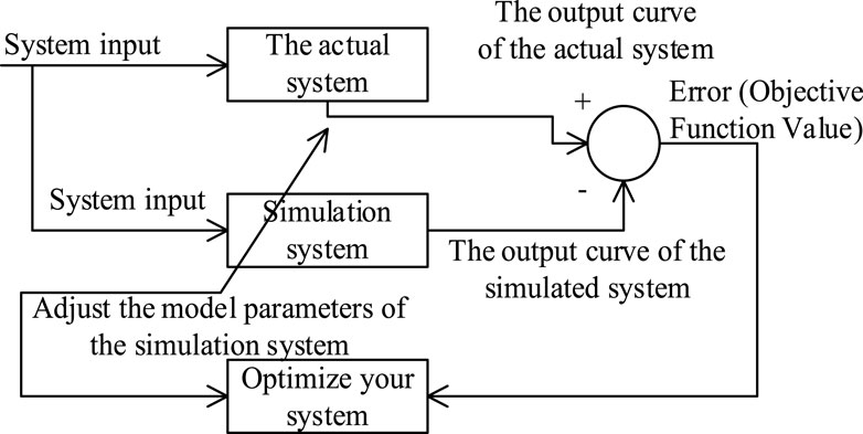
Figure 2. Schematic diagram of parameter identification system.
The system input in the above figure is voltage. In the actual system, this curve specifically showcases the accurately measured values of active and reactive power for the load. Similarly, the simulation system’s output curve mirrors this scenario, providing a simulated perspective on the active and reactive power of the load in response to voltage disturbance.
Initially, it is imperative to establish both the model structure and the objective function. Subsequently, the parameter identification process unfolds through the utilization of input and output data, employing an optimization method with the core principle of minimizing the objective function value. The central focus of this paper lies in defining the objective function, as articulated below Equation 6:
in the formula:
3.2 Dung beetle optimization algorithm (DBO)
The DBO algorithm specifically comes from the four living habits of DB, which are rolling, spawning, foraging and stealing. The Dung Beetle Optimizer (DBO) algorithm is a nature-inspired optimization technique based on the behavior of dung beetles. These insects exhibit unique foraging strategies that have been effectively translated into optimization algorithms to solve complex problems. The algorithm adapts the movement strategies of the dung beetles based on their success in finding good solutions. This adaptive mechanism enhances the efficiency of the search process. The principle diagram of the dung beetle optimization algorithm is shown in Figure 3, and the global optimal solution can be found after multiple iterations.
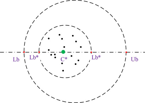
Figure 3. DBO algorithm schematic diagram.
3.2.1 Rolling DB
Rolling dung balls is a common behavior among dung beetles. These insects have a tendency to roll dung balls that are larger than their own size to their preferred location. During this rolling process, they utilize celestial cues, such as the Sun and Moon, to maintain a straight trajectory for the dung ball. The passage delineates the navigational conduct of a dung beetle within a designated search space. In order to replicate this behavioral phenomenon, adherence to a predetermined trajectory is imperative. This emulation is encapsulated within a formalized rolling mathematical model, wherein the dynamic repositioning of both the dung beetle and the concomitantly propelled ball undergo continuous updates throughout the rolling process. The rolling mathematical model is as follows Equation 7:
the current iteration times are denoted by t in the formula, where
1) In the optimization process, explore the entire problem space as fully as feasible.
2) Improved search performance, with less reliance on the local optimal.
When DB encounters obstacles that hinder its progress, it adopts a unique strategy akin to a dance to overcome the impediment and discover an alternative route. The essence of this method involves utilizing the tangent function to calculate a fresh roll direction, mirroring the intricate movements observed in a dance routine. Once the appropriate direction is determined, DB seamlessly continues its journey by rolling the associated ball backward. This dynamic approach constitutes the core of DB’s ability to adapt and navigate challenging environments. In essence, the process encompasses the update of DB’s position and establishes a comprehensive definition of its distinctive dance-like behavior Equation 8:
in the formula:
3.2.2 Spawning DB
Dung beetles show a fascinating behavior in nature. They carefully roll the dung balls, roll the cow dung into a dung ball with a diameter of about 2.5 cm, and quickly push it underground and bury it as the next-generation of food. This process is crucial for dung beetles (DB), as they carefully select a suitable spawning site to establish a safe habitat for the upcoming generation. The previous discussion underscored the importance of this behavior and motivated the introduction of boundary selection methods. This method is designed to simulate the specific area of female oviposition. The focus is on mimicking the natural conditions that ensure the safety and wellbeing of beetle offspring. The upper and lower limits of the selected region can be expressed by Formula 9:
where:
In the DBO algorithm, each female DB only lays a single egg per iteration to maintain ecological balance. This process prompts dynamic alterations in the boundary range of the spawning area, predominantly governed by adjustments to the R value. The determination of this R value may change at different stages of the iteration, thus affecting the size and shape of the spawning area. Therefore, in the whole iteration process, not only the number of eggs is regulated, but also the position of the hatching ball remains dynamic, evolving with the continuous adjustment of the boundary range. The specific position iteration formula can be articulated as follows Equation 10:
in the formula,
3.2.3 Foraging DB
The little DB that emerges from the breeding ball wants to feed, so we build the best foraging area and direct it there. The small DB’s position is updated in this way:
the ideal foraging area’s boundary division is shown above.
in the formula, the variables
3.2.4 Stealing DB
There are also some DBs who steal turds from other DBs. Furthermore, Eq. 11 shows that
in the formula,
3.3 The good point set
Nowadays, the initialization method of most swarm intelligence optimization algorithms is a random initialization form. The randomly generated population is unevenly distributed in the whole solution space. It is very gathered in some areas and scattered in others, resulting in the algorithm’s utilization of the entire search space not being high and the population diversity not being strong. Aiming at the problem of random initialization, many scholars have proposed and used good point-set initialization. The theory of the good point set originated from Hua Luogeng, a famous Chinese mathematician. The randomness of random initialization is too high, and there may be a phenomenon where the first-generation solution is very far from the optimal value. If the value of the first-generation solution is very close to the optimal value, it can not only improve the convergence speed but also the optimization accuracy under the premise of a certain number of iterations.
Using the good point set for initializing the population in optimization algorithms ensures uniform coverage of the search space, which improves the balance between exploration and exploitation, accelerates convergence, reduces bias, and enhances performance, particularly in high-dimensional spaces. This leads to more effective and efficient optimization, making it a preferred choice for initializing candidate solutions. To ensure population diversity and ergodicity, which can ultimately enhance the algorithm’s search performance, it is crucial to maintain a uniform distribution within the initial population. Achieving population diversity in DBO can be challenging due to the random selection of individuals during initialization.
A uniform and effective method for point selection is employed to initialize the population, aiming to address the aforementioned challenges, enhance population diversity, and optimize the utilization of the current solution. Leveraging the uniform distribution attribute of an excellent point set bolsters the flexibility and comprehensiveness of the population initialization process, enabling more thorough exploration of the solution space.
Currently, numerous clever algorithms (Cheng and Ding, 2020; Yan et al., 2023) have implemented the excellent point set initialization method with successful outcomes. The population’s initialization can be dispersed over the solution space by employing the good point set, which increases population variety and helps the algorithm find the globally optimal solution more effectively. The following is the principle: Let us assume that the person in the DBO algorithm is a point in n-dimensional Euclidean space, or, alternatively, that it is a position in the unit cube. When the number of individuals in a population exceeds the volume of the unit cube, it will cause individual repetition. The following actions can be performed to lower the repetition rate Equation 14:
in the formula:
in the formula: The top and lower boundaries of the
3.4 Algorithm flow
In this paper, the DBO algorithm enhanced by initializing the population with a good point set before updating the iterative position. The specific process is shown in Figure 4, which can be divided into seven steps:
Step 1: During the initial phase of the algorithm, a set of initial parameters is defined, serving as the starting point for subsequent optimization processes.
Step 2: Utilizing Formula 15, the algorithm initializes the population based on a pre-defined optimal point set, providing a well-founded starting configuration for the optimization process.
Step 3: By executing the objective function, the algorithm calculates fitness values for each dung beetle in the population, reflecting their performance at their current positions.
Step 4: Positions of all dung beetles are adjusted using a specified strategy to seek more optimal solutions. This step propels the population towards favorable directions.
Step 5: Examine the positions of each dung beetle to ensure they adhere to the defined problem boundaries, maintaining the problem’s feasibility and validity.
Step 6: In each iteration, it is essential to review and update the current optimal solution along with its corresponding fitness value to prevent the algorithm from disregarding potential global optima.
Step 7: Iterate through Steps 3 to 6 iteratively until the pre-defined termination criterion is satisfied. Upon termination, report the attained global optimal solution and its corresponding fitness value, concluding the entire optimization process.

Figure 4. GDBO Flowchart.
4 Case analysis
4.1 Algorithm initialization and parameter setting
The optimization algorithm’s parameter selection significantly impacts the optimization outcomes; hence, it is essential to meticulously choose optimal parameter values for simulation. Within each dung beetle colony, four distinct agents are present namely, the rolling ball DB, the spawning DB, the foraging DB, and the stealing DB. In the GDBO algorithm, the position vector of the i-th DB is represented by xi(t)=(yi1(t)
4.2 Measured data of a power plant and example simulation
To assess the efficacy of the DBO algorithm in the context of parameter identification for load modeling, this paper uses IDE, PSO, and GWO to identify the PMU measured data recorded by a power plant in Ruilijiang, Yunnan Province, at 10:14 on 20 November 2019, sampling once every 10 ms, for a total of 6,000 times. Figures 5, 6 illustrate the correlation between active and reactive power for both empirical and simulated datasets, respectively. The unit of each parameter is p.u.

Figure 5. Fitting diagram of active power identification.

Figure 6. Reactive power identification fitting diagram.
According to the above Figures 5, 6, it is not difficult to see that the DBO algorithm used in this paper is more accurate for the fitting value of parameter identification results and basically achieves coincidence. However, the traditional Dung Beetle Optimizer algorithm has a wide range for the first iteration of the initial population, resulting in a higher fitting value in the front, and then tends to be stable. Hence, the algorithm denominated as the Dung Beetle Optimizer, founded upon the well-defined point set articulated in this study, aptly addresses the aforementioned issue. The comparative outcomes pertaining to active and reactive power are visually presented in Figures 7, 8. The parameter values for identification derived through the application of the Dung Beetle Optimizer algorithm are delineated in Table 1.
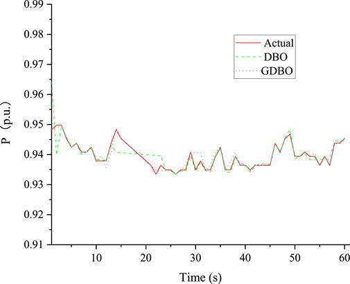
Figure 7. Comparison between active power DBO and GDBO.
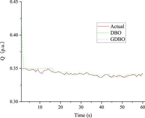
Figure 8. Comparison between reactive power DBO and GDBO.
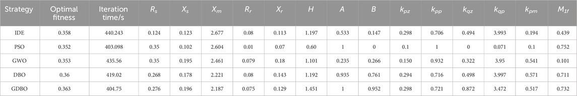
Table 1. Parameter identification results of measured data.
Figures 7, 8 show that the DBO algorithm based on the good point set has a faster initial iteration speed and can fit to the real value faster than the traditional DBO. The identification instances given above demonstrate that the DBO based on good point set has superior accuracy and speed than the other four algorithms in parameter identification of load modeling through a large number of practices.
4.3 Fitting effect evaluation
In this research, the assessment of fitting performance between observed data and simulated data relies on the utilization of specific metrics, namely the Mean Absolute Error (MAE) and the Root Mean Square Error (RMSE). These metrics serve as quantitative measures to evaluate the accuracy of the simulated data in comparison to the actual observations. The corresponding formulations for MAE and RMSE are precisely defined by Eqs 16, 17, respectively. By employing these metrics and their associated mathematical expressions, this study establishes a rigorous framework for quantifying the level of agreement or discrepancy between the simulated data and the observed data, thereby enhancing the precision and reliability of the evaluation process.
within the mathematical expression,
Compared with the traditional method, the improvement rates of the Mean Absolute Error (MAE) and the Root Mean Square Error (RMSE) of the method used in this paper are represented by
The assessment outcomes for the fitting efficacy of measured data using the GDBO algorithm, which relies on the proposed favorable point set in this study, along with comparisons to alternative algorithms, are presented in Table 2.
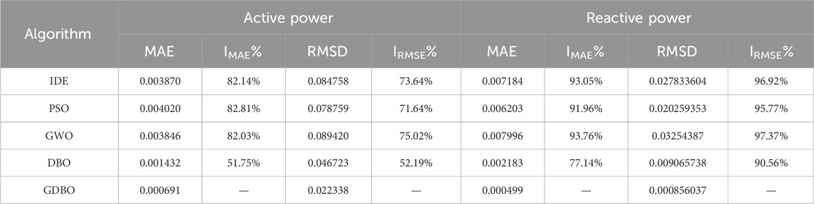
Table 2. Evaluation of model fitting effect.
Through a comparative analysis with alternative algorithms, upon careful examination, in the active power fitting, the GDBO algorithm used in this paper is compared with the IDE, PSO, GWO and traditional DBO algorithm in reducing the absolute average error, which is increased by 82.14%, 82.81%, 82.03%, and 51.75% respectively. In terms of reducing the root mean square error, the improvement rate of the GDBO algorithm also reached 73.64%, 71.64%, 75.02%, and 52.19%, respectively. At the same time, as shown in Table 2, the GDBO algorithm demonstrates remarkable performance when fitting reactive power applied to measured data of the model. Specifically, it exhibits the most minimal mean absolute error and root mean square error among the tested algorithms. This compelling observation underscores the superior efficacy of the proposed algorithm in the realm of parameter identification. The algorithm’s ability to minimize errors in fitting the measured data points to the model highlights its robustness and accuracy, signifying its potential as an effective tool in practical applications requiring precise parameter estimation. Moreover, the algorithm demonstrates increased robustness in the face of fluctuations in both active and reactive power.
5 Conclusion
DBO is utilized in this paper for load modeling and parameter identification. The results of the identification of load modeling reveal that DBO has a considerable improvement in accuracy and speed when compared to the other three methods. Consequently, DBO can be effectively utilized for parameter identification in load modeling, which can improve load modeling accuracy. Furthermore, the DBO method based on the good point set outperforms the classic DBO algorithm in terms of accuracy and speed, and gives a higher level of solution for parameter identification of load modeling.
Data availability statement
The original contributions presented in the study are included in the article/supplementary material, further inquiries can be directed to the corresponding author.
Author contributions
CX: Conceptualization, Validation, Writing–original draft, Writing–review and editing. XX: Conceptualization, Methodology, Writing–review and editing. XH: Methodology, Writing–review and editing. CD: Validation, Writing–review and editing.
Funding
The author(s) declare that financial support was received for the research, authorship, and/or publication of this article.
Conflict of interest
Authors CX, XX, XH and CD were employed by Electric Power Research Institute of Yunnan Power Grid Co., Ltd.
Publisher’s note
All claims expressed in this article are solely those of the authors and do not necessarily represent those of their affiliated organizations, or those of the publisher, the editors and the reviewers. Any product that may be evaluated in this article, or claim that may be made by its manufacturer, is not guaranteed or endorsed by the publisher.
References
Chen, H., Hao, R., Liu, Y., Wang, H., Wang, T., and Li, D. (2020). Parameter identification of time-varying power function load model based on improved RLS algorithm. High. Volt. Eng. 46 (07), 2380–2388. doi:10.13336/j.1003-6520.hve.20200310013
Cheng, M., and Ding, R. (2020). Multi-path coverage test case generation based on good-point set genetic algorithm. Comput. Digital Eng. 50 (09), 1940–1944. doi:10.3969/j.issn.1672-9722.2022.09.013
Diao, H., Li, P., Guo, S., Lin, S., Su, H., and Shen, Y. (2023). Parameter identification method for composite load model of PMU under small disturbance signal. Prot. Control Electr. Power Syst. 51 (13), 37–49. doi:10.19783/j.cnki.pspc.221680
Fang, C., Tang, X., Li, W., Zhang, N., Wei, X., and Chen, J. (2022). Optimal design of fast mechanical switches for 500 kV DC circuit breakers based on multi-strategy particle swarm optimization algorithm. High. Volt. Appar. 58 (01), 79–88. doi:10.13296/J.1001-1609.Hva.2022.01.011
Fu, W., Jiang, X., Li, B., Tan, C., Chen, B., and Chen, X. (2023). Rolling bearing fault diagnosis based on 2D time-frequency images and data augmentation technique. Meas. Sci. Technol. 34 (4), 045005. doi:10.1088/1361-6501/acabdb
Guo, C., Xie, H., Meng, X., He, P., Yang, L., and Wang, D. (2022). Parameter identification of load model based on grey wolf optimization algorithm. J. Electr. Power Sci. Technol. 37 (02), 30–37. doi:10.19781/j.issn.1673-9140.2022.02.004
Kang, P., Zhu, S., Wang, H., Fan, G., and Yang, G. (2021). Parameter identification of PV integrated load model based on improved butterfly algorithm. Renew. Energy 39 (11), 1541–1547. doi:10.13941/j.cnki.21-1469/tk.2021.11.018
Li, B., Gao, P., and Guo, Z. (2023). Improved dung beetle algorithm to optimize LSTM for photovoltaic array fault diagnosis. J. Electr. Power Syst. Automation, 1–10. doi:10.19635/j.cnki.csu-epsa.001317
Liu, Zi. (2007). Application of modern optimization algorithm in load model identification. Beijing: North China Electric Power University. doi:10.7666/d.y1058213
Pan, Z., and Bu, F. (2023). DV-Hop localization algorithm optimized by dung beetle algorithm [J/OL]. J. Electron. Meas. Instrum., 1–10. doi:10.13382/j.jemi.B2306338
Pattanaik, J. K., Basu, M., and Dash, D. P. (2017). Opposition-based differential evolution for hydrothermal power system. Prot. Control Mod. Power Syst. 2, 2. doi:10.1186/s41601-017-0033-5
Sheng, X., Ouyang, T., Yang, N., and Zhuang, J. (2021). Sample-based neural approximation approach for probabilistic constrained programs. IEEE Trans. neural Netw. Learn. Syst. 34, 1058–1065. doi:10.1109/TNNLS.2021.3102323
Swarupa, M. L., Kumar, V. G., Latha, K. S., Ravindra, M., and Kumar, B. P. (2024). Distribution state estimation and its impact of load modeling. Contemp. Math., 527–545. doi:10.37256/cm.5120242696
Wang, B., Huang, Y., Song, T., and Dong, J. (2011). Parameter identification of load model based on chaotic ant colony algorithm. Power Syst. Prot. Control 39 (14), 47–51. doi:10.3969/j.issn.1674-3415.2011.14.008
Wang, X., Sheng, X. K., Mu, K., and Wang, X. (2020). Research on electrical performance detection method of transformer oil based on multi-frequency ultrasonic technology and GWO-BP algorithm. High. Volt. Appar. 56 (08), 114–120. doi:10.13296/J.1001-1609.Hva.2020.08.018
Wang, Y., Gu, J., and Yuan, L. (2023). Distribution network state estimation based on attention-enhanced recurrent neural network pseudo-measurement modeling. Prot. Control Mod. Power Syst. 8, 31. doi:10.1186/s41601-023-00306-w
Wang, Y., Lu, C., and Zhang, X. (2019). Applicability comparison of different algorithms for ambient signal based load model parameter identification. Int. J. Electr. Power and Energy Syst. 111, 382–389. doi:10.1016/j.ijepes.2019.03.061
Wang, Z., Bian, S., Liu, X., Yu, K., and Shi, Y. (2014). Study on parameter identification of load model based on combination of chaos and quantum-behaved particle swarm optimization. Trans. China Electrotech. Soc. 29 (12), 211–217. doi:10.19595/j.cnki.1000-6753.tces.2014.12.027
Wu, P., Zhang, X., Lu, C., Wang, Y., Ye, H., and Ling, X. (2023). A composite load model aggregation method and its equivalent error analysis. Inter-national J. Electr. Power Energy Syst. 150, 109098. doi:10.1016/j.ijepes.2023.109098
Wu, Z., Fan, D., and Fan, Z. (2022). Traction load modeling and parameter identification based on improved sparrow search algorithm. Energies 15 (14), 5034. doi:10.3390/en15145034
Xu, J., Ma, J., Tang, Y., and He, R. (2009a). Parameter identification of load modeling based on improved differential evolution algorithm. Power Syst. Prot. Control 37 (24), 36–40 + 45. doi:10.3969/j.issn.1674-3415.2009.24.008
Xu, J., Ma, J., Tang, Y., and He, R. (2009b). Parameter identification of load modeling based on improved hybrid genetic algorithm. Mod. Electr. Power 26 (003), 23–27. doi:10.19725/j.cnki.1007-2322.2009.03.005
Xu, P., Fu, W., Lu, Q., Zhang, S., Wang, R., and Meng, J. (2023). Stability analysis of hydro-turbine governing system with sloping ceiling tailrace tunnel and upstream surge tank considering nonlinear hydro-turbine characteristics. Renew. Energy 210, 556–574. doi:10.1016/j.renene.2023.04.028
Xue, J., and Shen, B. (2022). Dung beetle optimizer: a new meta-heuristic algorithm for global optimization. J. Supercomput. 2022, 7305–7336. doi:10.1007/s11227-022-04959-6
Yan, S., Yang, P., Zhu, D., Wu, F., and Yan, Z. (2023). Improved sparrow search algorithm based on good point set. J. Beijing Univ. Aeronautics Astronautics, 1–13. doi:10.13700/J.BH.1001-5965.2021.0730
Yang, N., Dong, Z., Wu, L., Zhang, L., Shen, X., Chen, D., et al. (2022d). A comprehensive review of security-constrained unit commitment. J. Mod. Power Syst. Clean Energy 10 (No.3), 562–576. doi:10.35833/MPCE.2021.000255
Yang, N., Qin, T., Wu, L., Huang, Y., Huang, Y., Xing, C., et al. (2022c). A multi-agent game based joint planning approach for electricity-gas integrated energy systems considering wind power uncertainty. Electr. Power Syst. Res. 204, 107673. ISBN:0378-7796. doi:10.1016/j.epsr.2021.107673
Yang, N., Shen, X., Liang, P., Ding, L., Yan, J., Xing, C., et al. (2024). Spatial-temporal optimal pricing for charging stations: a model-driven approach based on group price response behavior of evs. IEEE Trans. Transp. Electrification, 1. doi:10.1109/TTE.2024.3385814
Yang, N., Yang, C., Wu, L., Shen, X., Jia, J., Li, Z., et al. (2022a). Intelligent da-ta-driven decision-making method for dynamic multisequence: an E-Seq2Seq-based SCUC expert system. IEEE Trans. Industrial Inf. 18 (No.5), 3126–3137. doi:10.1109/TII.2021.3107406
Yang, N., Yang, C., Xing, C., Ye, D., Jia, J., Chen, D., et al. (2022b). Deep learning-based SCUC decision-making: an intelligent data-driven approach with self-learning capabilities. IET Generation, Transm. Distribution 16 (No.4), 629–640. doi:10.1049/gtd2.12315
Yang, N., Ye, D., Zhou, Z., Cui, J., Chen, D., and Wang, X. (2018). Research on modelling and solution of stochastic SCUC under AC power flow constraints. IET Generation Transm. Distribution 12, 3618–3625. doi:10.1049/iet-gtd.2017.1845
Zhang, X., Lu, C., Lin, J., and Wang, Y. (2020). Experimental test of PMU measurement errors and the impact on load model parameter identification. IET Generation, Transm. Distribution 14 (20), 4593–4604. doi:10.1049/iet-gtd.2020.0297
Zhang, Y., Wei, L., Fu, W., Chen, X., and Hu, S. (2023a). Secondary frequency control strategy considering DoS attacks for MTDC system. Electr. Power Syst. Res. 214, 108888. doi:10.1016/j.epsr.2022.108888
Zhang, Y., Xie, X., Fu, W., Chen, X., Hu, S., Zhang, L., et al. (2023b). An optimal combining attack strategy against economic dispatch of integrated energy system. IEEE Trans. Circuits Syst. II Express Briefs 70 (1), 246–250. doi:10.1109/TCSII.2022.3196931
Zhou, D., Peng, X., Huang, X., Cheng, G., Tang, W., Zou, K., et al. (2023). Optimization method of power grid material warehousing and allocation based on multi-level storage system and reinforcement learning. Comput. Electr. Eng. 109, 108771. doi:10.1016/j.compeleceng.2023.108771
Zhu, B., Yang, Y., Wang, K., Liu, J., and Vilathgamuwa, D. M. (2023). High transformer utilization ratio and high voltage conversion gain flyback converter for photovoltaic application. IEEE Trans. Industry Appl. 60, 2840–2851. doi:10.1109/TIA.2023.3310488
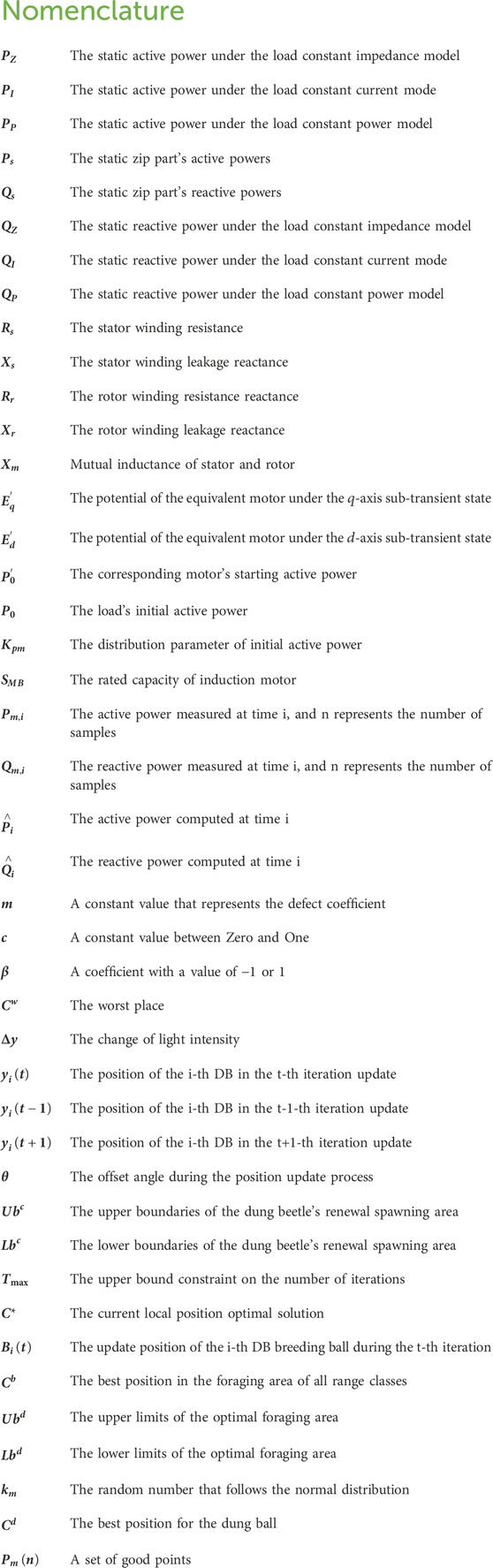
Nomenclature
Keywords: DBO algorithm, good point set, parameter identification, load modeling, electric power system
Citation: Xing C, Xi X, He X and Deng C (2024) Parameter identification method of load modeling based on improved dung beetle optimizer algorithm. Front. Energy Res. 12:1415796. doi: 10.3389/fenrg.2024.1415796
Received: 11 April 2024; Accepted: 19 July 2024;
Published: 20 August 2024.
Edited by:
Yitong Shang, Hong Kong University of Science and Technology, Hong Kong SAR, ChinaReviewed by:
Praveen Kumar Balachandran, Vardhaman College of Engineering, IndiaSomporn Sirisumrannukul, King Mongkut’s University of Technology North Bangkok, Thailand
Copyright © 2024 Xing, Xi, He and Deng. This is an open-access article distributed under the terms of the Creative Commons Attribution License (CC BY). The use, distribution or reproduction in other forums is permitted, provided the original author(s) and the copyright owner(s) are credited and that the original publication in this journal is cited, in accordance with accepted academic practice. No use, distribution or reproduction is permitted which does not comply with these terms.
*Correspondence: Chao Xing, eGluZ2NoYW9feW5AMTYzLmNvbQ==