Impacts of hydrogen on tropospheric ozone and methane and their modulation by atmospheric NOx

Atmospheric hydrogen concentrations have been increasing in recent decades. Hydrogen is radiatively inert, but it is chemically reactive and exerts an indirect radiative forcing through chemistry that perturbs the concentrations of key species within the troposphere, including ozone. Using the atmospheric version of the United Kingdom Earth System Model, we analyse the impact of 10% increased surface concentrations of hydrogen on ozone production and loss. We also analyse the impact of this hydrogen in atmospheres with lower anthropogenic emissions of nitrogen oxides (80% and 30% of present-day anthropogenic surface emissions), as this is a likely outcome of the transition from fossil fuels towards cleaner technologies. In each case, we also assess the changes in hydroxyl radical concentration and hence methane lifetime and calculate the net impact on the hydrogen tropospheric global warming potential (GWP). We find that the hydrogen tropospheric GWP₁₀₀ will change relatively little with decreases in surface anthropogenic NO_x emissions (9.4 and 9.1 for our present day and 30% anthropogenic emissions, respectively). The current estimate for hydrogen GWP₁₀₀ can therefore be applied to future scenarios of differing NO_x, although this conclusion may be impacted by future changes in emissions of other reactive species.

1 Introduction

Hydrogen and ozone are intricately linked in the atmosphere. Model simulations show that increases in atmospheric hydrogen concentrations, such as those observed in the past decade (Paulot et al., 2024), increase tropospheric ozone concentrations (Sand et al., 2023; Warwick et al., 2023), which in turn perturbs global temperature, because ozone is a greenhouse gas. It is therefore crucial to quantify the chemical mechanisms through which this change in tropospheric ozone with increase in hydrogen occurs.

Hydrogen can be added to the atmosphere through various routes. There can be leakages from the energy system, natural sources from soil and oceans, fossil fuel combustion, biomass burning and in situ chemical production from formaldehyde (Ehhalt and Rohrer, 2009). Atmospheric hydrogen can be removed by deposition to the ground, through biological activity (approximately 75% of hydrogen is removed by this route (Ehhalt and Rohrer, 2009)) or by reaction with other atmospheric species. Hydrogen reacts with a range of oxidants of which the most important is its reaction with OH:

$\text{OH}+{\mathrm{H}}_2\to {\mathrm{H}}_2\mathrm{O}+\mathrm{H}\left(\text{Reaction\hspace{0.17em}}1\right)$

The product hydrogen atoms rapidly oxidise to hydroperoxy radicals (HO₂), which are a critical component of ozone production (P(O₃)). Ozone is a greenhouse gas, and so, production of ozone by atmospheric hydrogen has an associated indirect global warming effect (Sand et al., 2023).

Hydrogen in the atmosphere also has impacts on tropospheric methane. Methane is impacted by hydrogen through Reaction 1 because OH is the primary oxidant for removal of methane through the following reaction:

${\text{CH}}_4+\text{OH\hspace{0.17em}}\to {\text{CH}}_3+{\mathrm{H}}_2\mathrm{O}\left(\text{Reaction\hspace{0.17em}}2\right)$

The reduction in OH concentrations brought about by additional H₂, because of the increased flux through Reaction 1, means there is less OH available to destroy methane. This increases the lifetime of methane in the troposphere.

Tropospheric P(O₃) occurs through the photolysis of NO₂ to yield NO and an oxygen atom, the latter of which rapidly reacts with O₂ to form O₃. Most emissions into the atmosphere of NO₂ gases (the collective term for both nitric oxide (NO) and nitrogen dioxide (NO₂) gases) is in the form of NO. It is the conversion of this NO to NO₂ by HO₂ through the reaction,

${\text{HO}}_2+\text{NO\hspace{0.17em}}\to {\text{NO}}_2+\text{OH\hspace{0.17em}}\left(\text{Reaction\hspace{0.17em}}3\right)$

that leads to ozone production (Crutzen, 1974) through the photolysis of NO₂, as explained above. The conversion of NO to NO₂ is also facilitated by organic peroxy radicals (RO₂) that are products (along with HO₂ radicals) in the oxidation of volatile organic compounds (VOCs) also emitted into the atmosphere. The primary link between hydrogen in the atmosphere and ozone production is therefore through Reaction 3. Since NO is a direct determinant of the rate of this reaction, we also explore in this paper the impact of different levels of atmospheric NO on the production of ozone from hydrogen.

The impact of Reaction 2, alongside a change in NO_x and CO was suggested by Schultz et al. (2003). As OH is produced through Reaction 3, lower NO_x will mean there is less OH present in the atmosphere. This was highlighted by Naik et al. (2013), whereby the change in NO_x emissions from the pre-industrial to present day (an increase of a factor of 3.19 ± 0.41) was associated with a 46.4% ± 12.2% increase in global mean OH.

The effects of changes to other atmospheric species alongside perturbations to hydrogen have been investigated in previous studies. These changes often represent the decrease in fossil fuel usage that is expected to occur alongside hydrogen energy production and are dependent on the structure of the final hydrogen economy. Warwick et al. (2004) found that when the removal of products from fossil fuel burning (NO_x, CO, methane and non-methane VOCs) are included, tropospheric ozone only increased a small amount. Similar conclusions were drawn by Schultz et al. (2003), in which hydrogen was increased while simultaneously decreasing NO_x and CO. Jacobson (2008) studied the changes to aerosol particles and cloud feedback with a full transition from fossil fuels to hydrogen scenario. Their results indicate that even with high hydrogen leakage rates (10%) many tropospheric pollutant levels improve. Most recently, Warwick et al. (2023) also investigated possible scenarios for changes in CO, CH₄, VOCs, and NO_x arising from a reduction in fossil fuel use alongside the hydrogen perturbation. In some cases, no change to NO_x was applied, on the basis that the change in NO_x will depend on how the hydrogen is used in a switch from fossil fuels to hydrogen. When hydrogen is combusted in air, thermal production of nitrogen oxides will still occur (Lewis, 2021). If hydrogen is used within a fuel cell, NO_x production through this route does not occur. Overall, Warwick et al. (2023) found that there were air quality benefits of switching to hydrogen, but that the change in ozone was minimal between the different replacement scenarios. Our paper aims to decouple the impact that NO_x has on this relationship between hydrogen and ozone.

There are also stratospheric effects of hydrogen on both ozone and water vapour (Forster et al., 2007), but in this paper, we only discuss the troposphere.

Overall, these previous studies have explored the changes that ensue when hydrogen is emitted alongside decreases in the pollutants which are associated with the hydrogen. They have not quantified the impact of hydrogen alone when there are different background levels of an individual pollutant, such as NO_x. Therefore, in this paper, the relationship of hydrogen with NO_x is analysed.

2 Methods

2.1 Model set-up

The United Kingdom’s Earth System Model Atmosphere Only (UKESM1 Atmosphere Only) configuration at version 11.1 with StratTrop chemistry was used for these experiments. This model has grid cells of size 1.88° × 1.25° (longitude × latitude). The model has 85 height levels between the surface and 85 km, non-linearly spaced. A detailed chemical model description is given by Archibald et al. (2020). Input emissions include the species C₂H₆, C₃H₈, CO, HCHO, (CH₃)₂CO, CH₃CHO, NO and other non-methane VOCs. Methane and hydrogen in this configuration are lower boundary condition species for which the surface mixing ratios are prescribed.

The model is set up to run with an aerosol climatology (instead of the standard interactive aerosols), with emissions of all species fixed to the year 2010. Water vapour concentrations have been decoupled from the chemistry and instead respond to a fixed methane oxidation rate. Radiation is also decoupled from chemistry. These changes have been made to ensure that the meteorological conditions are identical in each run and therefore that any changes observed are due to chemical perturbations driven by changes in emissions or perturbed lower boundary conditions, and not to changes in meteorology. This configuration allows the study to be able to see small percentage changes in fields which would usually be obscured by changes to model dynamics in the standard set-up. Decoupling the radiation from the chemistry means that any perturbations to radiatively active species by hydrogen will not alter the temperature of the atmosphere. If the temperature was free to respond, there would be small influences on reaction rates and transport and therefore on species concentration.

We have developed a new technique to incorporate temporally and latitudinally varying lower boundary conditions for hydrogen and methane. Lower boundary conditions in the model involve forcing the concentration of the species in the surface level of the model at each dynamical time-step. The species is then able to mix into the troposphere and react as a tracer, but the forcing prevents the surface mixing ratio from developing. The original configuration of this model uses a single global value for the surface lower boundary condition for hydrogen. Although the new technique still faces the issues highlighted above, this is an improved representation of surface hydrogen and methane.

The new lower boundary condition input for “present day” hydrogen uses the volume mixing ratios for 2010 from the National Oceanic and Atmospheric Administration Global Monitoring Laboratory, which were smoothed to create a monthly and latitudinally varying profile by Sand et al. (2023). The surface profile for hydrogen has an interhemispheric gradient of higher mixing ratios in the Southern Hemisphere than the Northern Hemisphere (Ehhalt and Rohrer, 2009). The profile also has a seasonal cycle (Figure 1). Representing the hydrogen surface profile with latitudinal and temporal variation is therefore needed to capture these characteristics. This methodology can be extended for any lower boundary condition species in the model. For methane (Figure 1), the 2010 CMIP6 input4mip data was used (Meinshausen et al., 2017).

Figure 1

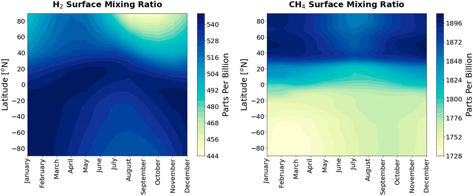
Figure 1. Lower boundary condition input mixing ratios for hydrogen (left) and methane (right) in parts per billion (ppb). Both are shown as latitude against time and are input as a monthly varying annual file.

In the model, hydrogen takes part in seven chemical reactions. Three of these are production reactions, and four are loss reactions:

$\text{HCHO}+\mathrm{h}\mathrm{\nu }\to {\mathrm{H}}_2+\text{CO\hspace{0.17em}}\left(\text{Reaction\hspace{0.17em}}4\right)$

${\text{HO}}_2+\mathrm{H}\to {\mathrm{H}}_2+{\mathrm{O}}_2\left(\text{Reaction\hspace{0.17em}}5\right)$

${\mathrm{O}}^1\mathrm{D}+{\text{CH}}_4\to \text{\hspace{0.17em}HCHO}+{\mathrm{H}}_2\left(\text{Reaction\hspace{0.17em}}6\right)$

${\mathrm{O}}^1\mathrm{D}+{\mathrm{H}}_2\to \text{\hspace{0.17em}OH}+\mathrm{H}\left(\text{Reaction\hspace{0.17em}}7\right)$

${\mathrm{O}}^3\mathrm{P}+{\mathrm{H}}_2\to \text{\hspace{0.17em}OH}+\mathrm{H}\left(\text{Reaction\hspace{0.17em}}8\right)$

$\text{OH}+{\mathrm{H}}_2\to {\mathrm{H}}_2\mathrm{O}+{\text{HO}}_2\left(\text{Reaction\hspace{0.17em}}1*\right)$

$\text{Cl}+{\mathrm{H}}_2\to \text{\hspace{0.17em}HCl}+\mathrm{H}\left(\text{Reaction\hspace{0.17em}}9\right)$

Reaction 1* produces hydroperoxy radicals (HO₂), rather than H as in Reaction 1.

2.2 Description of model runs

Nine experiments were run, comprising three experiments that focus on changes to surface hydrogen and methane, repeated at each of the following three levels of anthropogenic NO_x emissions:

1. “HighNO Atmosphere” = 100% anthropogenic surface NO_x emissions compared to 2010

2. “MidNO Atmosphere” = 80% anthropogenic surface NO_x emissions compared to 2010

3. “LowNO Atmosphere” = 30% anthropogenic surface NO_x emissions compared to 2010

For each of the HighNO, MidNO and LowNO cases, the following three experiments have been run (following Sand et al., 2023):

1. _Base: Baseline CH₄ and H₂ lower boundary condition

2. _H2: Baseline CH₄ lower boundary condition, 10% additional surface H₂ lower boundary condition

3. _CH4: Baseline H₂ lower boundary condition, 10% additional surface CH₄ lower boundary condition

The magnitudes of the hydrogen perturbation and NO_x emissions are based on potential 2040s futures. The assumption for the _H2 experiments that hydrogen will increase by an additional 10% (compared to 2010) by the mid-2040s is derived from the average rate of increase of hydrogen given by Patterson et al. (2021), between measurements in 1852 and modern-day measurements. Realistically, this change will not have a uniform global distribution but instead may be focused on areas of current anthropogenic energy production. This experiment is idealised and perturbs hydrogen over the whole surface. This perturbation is a simple scaling factor applied to the hydrogen surface profile. Patterson et al. (2021) also suggest a more complex mechanism for the hydrogen increase which changes over time. Based on this rate of increase, a 10% increase in hydrogen from 2010 would occur around a decade earlier.

The methane perturbation runs (_CH4) are necessary in order to calculate the impact of hydrogen on methane, as the methane is fixed in these experiments (Sand et al., 2023). The choice of a 10% surface perturbation in methane matches that used by Sand et al. (2023), in the models which were run with lower boundary conditions for hydrogen and methane, but the exact magnitude is not important as the outputs from these experiments are scaled.

The different levels of anthropogenic NO_x emissions for our simulations have been chosen based on CMIP6 scenarios for these emissions in the 2040s. Using the Community Emissions Data System (CEDS) (Riahi et al., 2017; Gidden et al., 2019), we can calculate anthropogenic NO_x emissions in the CMIP6 Emissions Scenarios Input Data relative to 2010 (the latter based on the historical emissions of van Marle et al. (2017) and Hoesly et al. (2018)). This data has surface anthropogenic global emissions of NO_x from the sources: Agriculture, Energy Sector, Industrial Sector, International Shipping, Residential Commercial Other, Transportation and Waste. Elevated anthropogenic NO_x emissions (aircraft emissions) have not been perturbed in these experiments. From comparison of the total NO_x emissions in the mid-2040s to the historical 2010 emissions, a globally uniform scaling factor on the 2010 emissions file can therefore be applied to represent this decrease.

There are nine CMIP6 scenarios available to inform the range of changes which may occur to anthropogenic NO_x emissions. Broadly, NO_x emissions in the 2040s in these scenarios span the range of 30%–110% of the NO_x emitted in 2010. Taking the emissions of van Marle et al. (2017) and Hoesly et al. (2018) for 2010 to represent present-day atmosphere, the scenarios SSP3-70, SSP5-34-OS and SSP5-85 in the 2040s are well represented by this level of NO_x. Therefore 100% present-day NO_x is what we use for our HighNO experiments. A cluster of CMIP6 scenarios have 2040s NO_x emissions near to the value of 80% of the 2010 emissions and therefore this is used for our MidNO experiments. The lower end of the CMIP6 NO_x emissions (∼30% of present) occurs in the SSP1-19 scenario. Therefore, 30% anthropogenic NO_x emissions are used in our LowNO experiment. In the more complex hydrogen increase scenario of Patterson et al. (2021), where the 10% increase in hydrogen occurs a decade earlier, our LowNO scenario is probably unlikely and instead a lower limit for the associated change in anthropogenic NO_x emissions would be higher. Our experiments have not accounted for regional variations in future NO_x distributions.

Note that for descriptive convenience, we use the notation “HighNO” etc. to refer to our model experiments using different anthropogenic NO_x emissions. Emissions of NO_x are input to the model as the species NO.

Each experiment was run for 15 years to allow the model to spin up to an equilibrium state, with meteorology that varies over this time period (but is identical between the runs). Meteorology varies based on sea ice and sea surface temperature inputs. The radiation scheme reads fixed values for the radiatively active species. The final year of the experiments is analysed.

2.3 Explanation of the methane perturbed configuration

The experiments are run with a methane lower boundary condition. When hydrogen is perturbed in the _H2 experiments, a change in methane is expected, due to the decreased OH concentrations. This leads to less removal of methane through Reaction 2. However, because of the forced lower boundary condition, only a very small perturbation in the total model methane burden is modelled in the _H2 runs. The same methane lower boundary condition is used in the HighNO, MidNO and LowNO base runs and so, implicitly assume different CH₄ emissions.

To capture the full impact that the hydrogen perturbation has on methane, the methane perturbation run is used. To scale this 10% methane perturbation to the actual change we expect from the increased hydrogen, Equation 1 is applied (Sand et al., 2023). The equation scales the 10% change in methane by this factor, which represents the size of the expected change in methane in the hydrogen perturbation run. This is calculated using a methane stratospheric lifetime of 120 years and a lifetime to loss to soil of 160 years. The methane loss from OH is used, with the stratosphere masked off using the model’s own tropopause diagnostic (not including the tropopause level).

$H2\_effect\_on\_CH4=CH4\_effect\ast CH4\_flux\_per\_H2\_flux\ast \frac{H2\_burden\_change\left[\_H2-\_Base\right]}{CH4\_burden\_change\left[\_CH4-\_Base\right]}(1)$

These terms are defined in the figure caption of Supplementary Figure S2 of Sand et al. (2023).

The total impact of hydrogen on the atmosphere is therefore the direct change from hydrogen in _H2 added to the scaled change caused by methane in _CH4. This is done using a global number for the methane effect, calculated separately for each NO_x scenario.

As our experimental set-up has fixed methane surface mixing ratios, we must use the methane lifetime to infer the change in methane which would be observed. The methane lifetime is calculated using the method from Stevenson et al. (2013) and Sand et al. (2023) (summarised as Equations 2, 3 below):

$C{H}_4+OHLifetime\left(a\right)=\frac{WholeAtmosphericC{H}_{4}Burden\left(Tg\right)}{TroposphericLossFluxThroughC{H}_4+OH\left(Tg{a}^{-1}\right)}(2)$

$TotalC{H}_{4}Lifetime\left(a\right)={\left(\frac{1}{TroposphericC{H}_4+OHLifetime\left(a\right)}+\frac{1}{StratosphericC{H}_{4}Lifetime\left(a\right)}+\frac{1}{SoilC{H}_{4}Lifetime\left(a\right)}\right)}^{-1}(3)$

3 Results and discussion

3.1 The impact of additional hydrogen in present-day atmosphere

3.1.1 Species changes

Additional atmospheric hydrogen perturbs other chemical species via the seven reactions modelled in UKESM1 listed above. Figure 2 shows the zonal annual mean changes in the abundances of the key species that change following addition of hydrogen, including the effect of the induced changes in methane from the methane perturbed run. A decrease is observed in the OH mass mixing ratio due to an increased flux through Reaction 1*. Reaction 1* produces HO₂. Ozone production is related to HO₂ through Reaction 3r; therefore, as HO₂ increases, so does ozone.

Figure 2

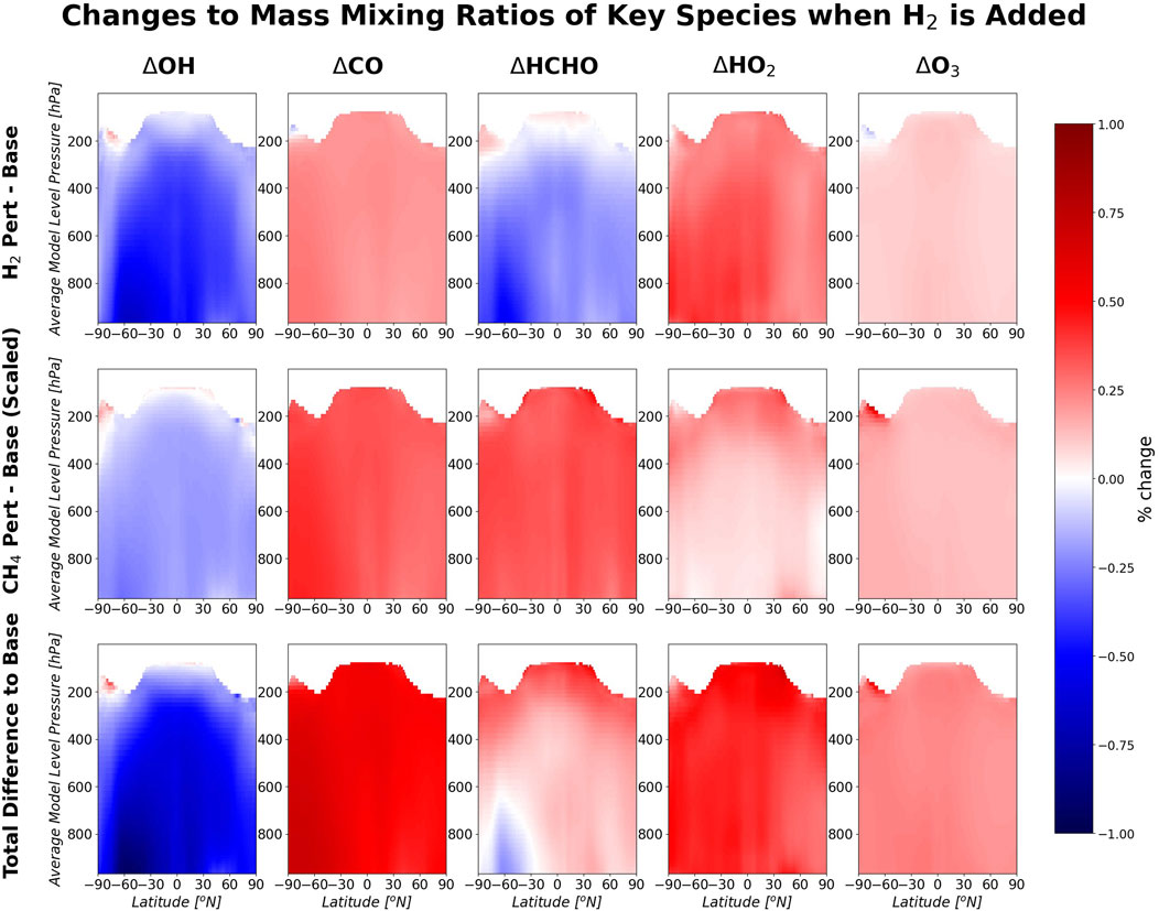
Figure 2. Zonal annual mean percentage change in atmospheric species mass mixing ratios between the base scenario and the scenario with a 10% increase in H₂. The methane effect is included here by applying the methane factor to the change in the species. Column 1 is the change in hydroxyl, 2 is the change in carbon monoxide, 3 is the change in formaldehyde, 4 is the change in hydroperoxy radical and 5 is the change in ozone. Row 1 is the change in the species due to hydrogen perturbation directly, row 2 is the change in the species due to the impact of hydrogen on methane and row 3 is the combined effect of hydrogen and methane (due to hydrogen) on the species. These are plotted against the average pressure of each model level in the troposphere, which is an approximation of pressure.

Overall, there is an increase in formaldehyde (HCHO) mixing ratios throughout the troposphere following an increase of hydrogen in the model. There are regions of decreased HCHO concentration in the southern hemisphere low troposphere. Figure 2 apportions the change in HCHO between the hydrogen perturbed run and the methane perturbed run. In the hydrogen perturbed run, HCHO decreases throughout much of the troposphere. In the methane perturbed run, HCHO increases throughout the troposphere. Methane is a precursor for HCHO. The total effect is the summation of the responses in the two perturbations.

Hydroxyl is the major oxidant for carbon monoxide (CO). Therefore, lower OH leads to reduced loss of CO and therefore to higher concentrations of CO. CO is produced by multiple routes (Zheng et al., 2019) which will each respond differently to a hydrogen perturbation. The net effect is an increase in CO throughout the troposphere.

3.1.2 The ozone budget

Additional atmospheric hydrogen leads to a positive perturbation in tropospheric ozone. The causes of the change in tropospheric ozone following the addition of hydrogen can be investigated by analysing the fluxes through the reactions that affect the ozone concentration change (the chemical budget).

The O_x chemical budget describes the major reactions that produce and remove O_x (O + O₃) in the atmosphere. In the base scenario, the O_x loss is dominated by H₂O + O¹D, O₃ + HO₂ and OH + O₃ (51.8%, 30.9%, and 14.0% respectively) and the production is dominated by NO + HO₂, NO + MeOO, and NO + RO₂ (66.1%, 22.4%, and 9.0%) (Figure 3). Total tropospheric ozone chemical production in the base is 6,000 Tg O₃ a⁻¹ and total tropospheric ozone chemical loss is 4,980 Tg O₃ a⁻¹.

Figure 3

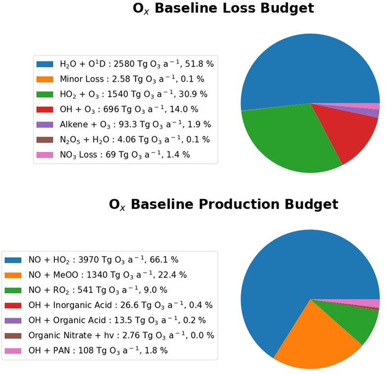
Figure 3. Pie chart of the O_x chemical budget in the HighNO_Base scenario. The top and bottom panels show the relative fluxes through the O_x loss and the O_x production reactions respectively. The legend details the reactions, the absolute magnitude of fluxes in Tg O₃ a⁻¹ (rounded to three significant figures) and the percentage contribution of each term.

This ozone budget compares well with that reported in Warwick et al. (2023), which has total ozone chemical production of 5,856 Tg a⁻¹ and total ozone chemical loss of 4,942 Tg a⁻¹.

Figure 4 shows that when 10% additional atmospheric hydrogen is added to the model, these O_x budget terms are perturbed only very slightly from the base.

Figure 4

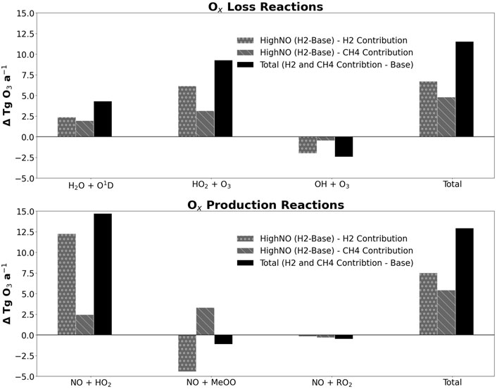
Figure 4. Bar chart showing the changes in the O_x chemical loss fluxes (top panel) and production fluxes (bottom panel) relative to base. The black bar is the absolute change with the grey bars apportioning the absolute change into the contribution from hydrogen (dotted grey) and the contribution from methane (striped grey). Only the three major loss and production reactions are shown, as these make up 97% of the total loss and production. The final set of bars on each chart show the changes in total O_x loss (top) and total O_x production (bottom) from all O_x budget reactions, not just the major reactions.

The flux of all the loss reactions increases, except for direct loss of ozone by OH (−2.4 Tg O₃ a⁻¹). The flux through OH + O₃ presumably decreases because of the decreased annual average tropospheric OH concentration. The fluxes through the other six loss reactions increase in response to the chemical changes to the key species already discussed. Fluxes through H₂O + O¹D and HO₂ + O₃ have changed to a much larger extent than for the other 4 loss reactions and thus have a greater impact on the ozone. Direct loss by HO₂ has increased (+9.3 Tg O₃ a⁻¹) because annual average HO₂ concentration has increased; and H₂O + O¹D has increased (+4.3 Tg O₃ a⁻¹) because ozone photolysis in the troposphere produces O¹D, so with greater ozone we expect more O¹D. However, the latter is complicated by the fact that destruction of methane and hydrogen by O¹D also occurs.

The striped, grey bars in Figure 4 also show the changes in the ozone production and loss reactions that are induced through the increases in methane that arise from 10% increase in H₂. For all the loss reactions, the methane-induced fluxes are in the same direction as the hydrogen-induced fluxes. Therefore, the total loss of ozone increases, as the compensation by the decreased loss through OH + O₃ is not sufficient to offset the increased losses through other loss processes.

For the production reactions, the change is dominated by the changes in fluxes through NO + HO₂ and NO + MeOO, with a minor contribution from NO + RO₂. This aligns with these being the three principal reactions in the O_x production budget. The increase in flux through NO + HO₂ (+14.7 O₃ Tg a⁻¹) is due to the increase in HO₂ concentration. The relative change in production fluxes is greatest for the reaction OH + Inorganic Acid; however, as this reaction is only a minor constituent of the O_x budget, it does not have a major impact on the overall change in ozone.

Overall, the change in chemical production and loss of O_x (+12.9 Tg O₃ a⁻¹, +11.5 Tg O₃ a⁻¹) following hydrogen perturbation are positive.

The methane perturbation experiment perturbed most of the ozone budget reactions in the same direction as the hydrogen perturbation experiment, albeit to different magnitudes (results not shown). This further confirms the similarity between the chemical behaviours of methane and hydrogen. The consequences of the perturbations on the reaction between NO and MeOO differ, however. This flux change is strongly positive for an increase in methane, but negative for an increase in hydrogen. Methane is a precursor for MeOO. Separating these hydrogen perturbation and methane perturbation effects is not realistic. However, observing the different responses in each experiment gives insight into how these budget terms change.

Our results for the hydrogen perturbation are compared in Table 1 with those from Warwick et al. (2023). They report changes to the following ozone budget terms under different hydrogen lower boundary condition experiments: HO₂ + NO, NO + MeOO, HO₂ + O₃, OH + O₃, total P(O₃) and total L(O₃). They ran multiple perturbation experiments where surface hydrogen was increased globally and included the methane feedback for the hydrogen increases of 1000 and 1500 ppb (1500H2_CH4f and 2000H2_CH4f). Here, we scale down the perturbations in these ozone budget terms to each match what might be expected for a 10% change, under the assumption that the change in flux is linear in each case. Table 1 shows the range of flux differences calculated from the Warwick et al. scenarios. Most of the budget terms are similar between this work and Warwick et al. but our work produces a slightly larger flux change in all cases.

Table 1

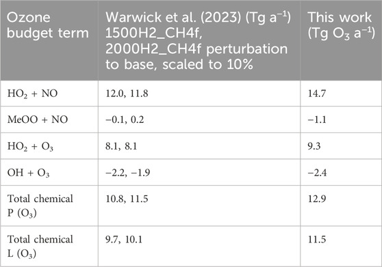
Table 1. Comparison of ozone budget terms in this work to Supplementary Table S2 in Warwick et al. (2023) for their scenarios 1500H2_CH4f and 2000H2_CH4f. The latter have been scaled down to a 10% increase to compare with this work.

Spatially, the fluxes through the five primary reactions that contribute to the change in ozone all change most through the tropics and the lower tropical troposphere (Figure 5). The increase is governed by the increased flux through HO₂ + NO, which is also the only reaction of those in Figure 5 that shows a clear perturbation in the upper tropical troposphere (UTT). The ozone radiative effect is not uniform throughout the troposphere, with the greatest warming occurring in the UTT (Rap et al., 2015). The change in HO₂ + NO in this region is therefore crucial for understanding the warming impact of the increased ozone under this hydrogen perturbation scenario.

Figure 5

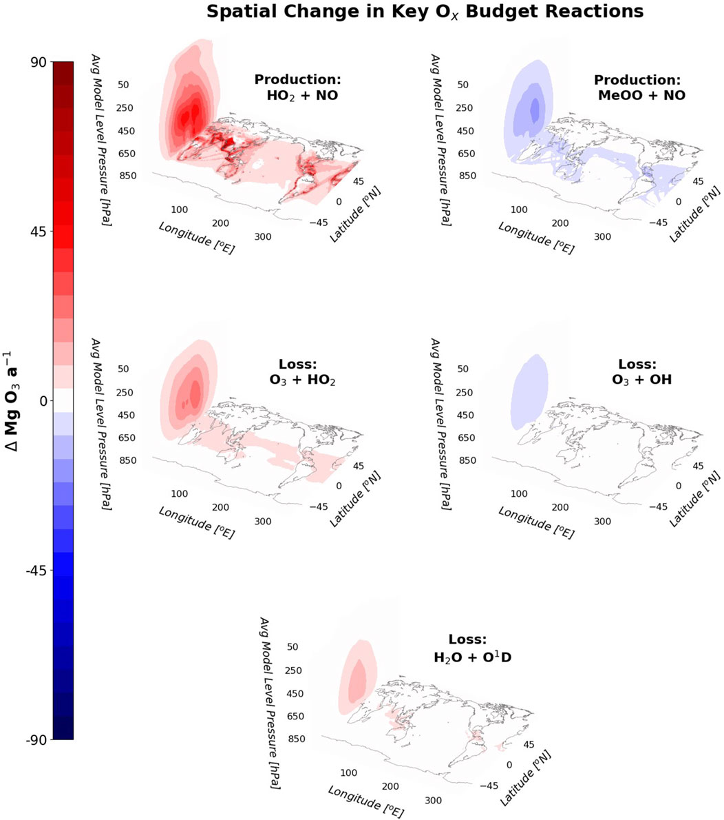
Figure 5. Spatial changes in the fluxes through the five primary O_x budget reactions for a 10% increase in H₂ (including the indirect impact of the H₂ change on methane) visualised as a zonal annual mean vertical profile (left panel in each plot) and an annual mean surface concentration (global maps). The z axis is the average pressure of each model level in the troposphere, which is an approximation of pressure. The changes are shown in Mg O₃ a⁻¹.

3.2 The impact of additional hydrogen in potential future atmospheres

3.2.1 Changing anthropogenic emissions impact in HighNO, MidNO, and LowNO atmospheres

In these simulations, only anthropogenic surface emissions of NO_x have been changed. There are additional sources of NO_x through aircraft emissions, biomass burning emissions, soil emissions and lightning. Some of the NO_x may also be converted to long-lived species such as peroxyacetyl nitrate. Therefore, a decrease of 20% in NO_x anthropogenic emissions will not change total tropospheric NO_x concentrations by 20%. In addition, the anthropogenic NO_x emissions are not spatially uniform, being considerably more abundant in the northern hemisphere, so the response to a decrease in anthropogenic NO_x emissions is therefore also spatially varied.

The annual average tropospheric NO burdens in the base MidNO and LowNO scenarios are approximately 87% and 64% of the tropospheric NO burden in the base HighNO scenario, respectively. Spatially, we observe a decrease in tropospheric NO in the MidNO and LowNO scenarios compared to the HighNO scenarios. This change is focused on the lower tropospheric northern hemisphere.

The model’s advection scheme sometimes redistributes a small proportion of the mass in an unphysical manner for experiments with emissions perturbations at the surface. This leads to some regions, particularly in the southern hemisphere upper troposphere, where the change in NO_y is negative in the HighNO scenario compared to the MidNO and LowNO scenarios (the reason for this issue is under active investigation by the code owners, but it is related to advection and not chemistry). To account for this in the GWP calculations, any gridcell in which NO_y volume mixing ratio in the HighNO experiment is less than in the MidNO or LowNO experiments is discounted (∼11% of all tropospheric gridcells). In these gridcells, the HighNO equivalent run is added (the base run for all base scenarios etc.) to yield a full dataset for the GWP calculations. This should minimise the impact of these gridcells. NO_y is defined here as NO, NO₂, N₂O₅, NO₃, HONO₂, HO₂NO₂, PAN, and ISON with the UKCA defined molar masses.

3.2.2 Chemical differences when hydrogen is added to HighNO, MidNO, and LowNO atmospheres

Figure 6 shows the changes in tropospheric burdens of OH, HO₂ and O₃ for a 10% increase in hydrogen compared with no hydrogen perturbation for the LowNO, MidNO, and HighNO atmospheres. There is a greater negative perturbation to OH when hydrogen is added to the HighNO atmosphere than when it is added to the MidNO and LowNO atmospheres. More OH is present in the atmosphere when NO is higher as NO produces OH through Reaction 1*. In the LowNO atmosphere, less OH is available to react with the hydrogen, and so, for the same amount of hydrogen added, the flux through OH + H₂ is lower and the change in OH is smaller.

Figure 6

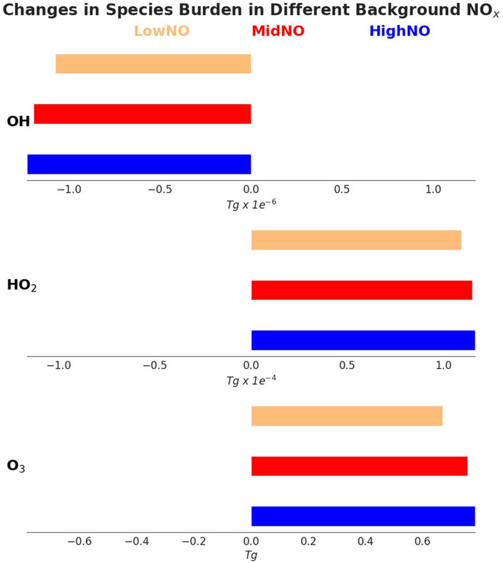
Figure 6. The absolute changes in tropospheric burdens of OH, HO₂, and O₃ for a 10% increase in H₂ compared to no H₂ perturbation, including the methane induced component. The different colours show the burden changes for the HighNO (blue), MidNO (red), and LowNO (green) scenarios. A negative value indicates that the tropospheric average annual burden of that species has decreased and a positive value indicates an increase.

For HO₂, the elevation in burden is greatest when the hydrogen is added to the HighNO atmosphere and least when it is added to the LowNO atmosphere (Figure 6). This is consistent with the larger negative perturbation of OH in higher NO versus lower NO atmospheres. This leads to a greater increase in HO₂ through the increased flux of reaction of OH + H₂. The greater HO₂ also means that more ozone is produced in higher NO atmospheres.

The ozone produced in the HighNO atmosphere when hydrogen is perturbed increases by a slightly higher percentage in the Southern Hemisphere than in the Northern Hemisphere. This may be caused by the approach of increasing hydrogen by 10% across the surface, hence adding more hydrogen to the Southern Hemisphere where concentrations are greater. When anthropogenic NO_x emissions are perturbed (primarily in the Northern Hemisphere), the overall influence of hydrogen perturbation on ozone may be influenced by these latitudinal dependencies. The experimental design does not allow for these dependencies to be explored further.

3.2.3 Changes to the ozone budget in HighNO, MidNO, and LowNO atmospheres

The changes in the ozone budget are determined by the five key O_x budget reactions through which hydrogen interacts with ozone (H₂O + O¹D, O₃ + HO₂, OH + O₃, NO + HO₂, and NO + MeOO). In every case there is a smaller change in flux through the reaction in the LowNO atmosphere compared with the MidNO and HighNO atmospheres, indicating that the magnitude of the change for ozone is reduced in the lower NO_x atmospheres. The spatial distribution of these changes is similar for HighNO, MidNO, and LowNO atmospheres. This is because the spatial distribution of the NO_x emissions has not been altered between the scenarios, only scaled. It is possible that spatial changes in future NO_x emissions may yield a slightly different result. For ozone production, the flux change is dominated by the NO + HO₂ reaction, whereas for ozone loss the change is primarily in the HO₂ + O₃ reaction. This indicates that the greatest impact of additional hydrogen on ozone is through HO₂, which is related to NO through NO + HO₂.

3.2.4 Changes to methane following hydrogen perturbation in HighNO, MidNO, and LowNO atmospheres

The other crucial species to understand in these scenarios is methane. When hydrogen is added to the atmosphere, reaction of OH with the hydrogen means less OH is available to react with methane. This extends the methane lifetime. Less methane is removed by OH in the LowNO and MidNO base atmospheres than in the HighNO base atmosphere. This is observed in the tropospheric CH₄ + OH flux rates (Figure 7). For example, the MidNO_Base CH₄ + OH flux is 18.9 Tg a⁻¹ smaller than the equivalent HighNO flux. The methane lifetime is therefore longer in the MidNO and LowNO atmospheres than in the HighNO atmosphere (Figure 7).

Figure 7

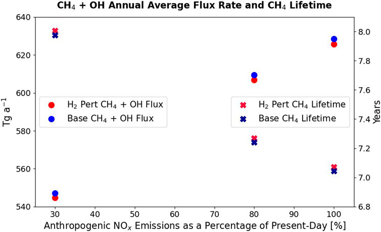
Figure 7. Circles (left hand axis): Tropospheric methane loss flux through reaction with OH in the perturbed hydrogen runs (not including the indirect methane effect) and in the _Base experiments for the HighNO, MidNO, and LowNO levels of atmospheric NO_x (which are expressed as a % of present-day NO_x). Crosses (right hand axis): The corresponding total methane lifetimes.

When hydrogen is added to each of the atmospheres, the OH is reduced and so the CH₄ + OH flux is lower than in the _Base experiment. Less OH has been removed by the same perturbation of hydrogen in the Low NO and MidNO atmospheres than in the HighNO atmosphere. The flux difference between the HighNO_Base to hydrogen perturbation experiment (not including the methane adjustment) is 2.73 Tg a⁻¹, while in the MidNO atmosphere the difference it is 2.65 Tg a⁻¹ and in the LowNO atmosphere it is 2.39 Tg a⁻¹ (Figure 7). Therefore, the direct impact of hydrogen on methane destruction is smaller in the LowNO and MidNO atmospheres, than in the HighNO atmosphere. This is consistent with the differences observed in the OH tropospheric burdens (Figure 6).

3.3 Hydrogen tropospheric global warming potential in present-day and potential future atmospheres

3.3.1 Methane

The hydrogen global warming potential due to methane can be calculated from the tropospheric CH₄ + OH flux in the base (_Base), hydrogen perturbation (_H2) and methane perturbation (_CH4) experiments. The hydrogen absolute global warming potential due to methane can be converted into a global warming potential over a 100-year time horizon (GWP₁₀₀) by dividing the value by the CO₂ GWP₁₀₀.

The total deposition flux of hydrogen has been fixed here to 57 Tg a⁻¹ for the _Base experiments and to 62.7 Tg a⁻¹ for the _H2 experiments. The former value is the model mean soil sink from Sand et al. (2023), with a 10% scaling applied for the _H2 experiments. Table 2 presents the total hydrogen GWP due to hydrogen’s impact on methane, as calculated in this work for the HighNO, MidNO, and LowNO atmospheres.

Table 2

Table 2. Values for the hydrogen GWP₁₀₀ due to changes in methane in the hydrogen perturbation experiments in the HighNO, MidNO, and LowNO atmospheres.

The hydrogen tropospheric GWP₁₀₀ contributions from methane are very similar in all three of the atmospheres of differing NO_x levels. The extended methane lifetime also causes a change to the stratospheric water vapour and stratospheric ozone concentrations, neither of which are retrievable in our experiments.

The methane GWP is calculated via multiplication of the methane flux per hydrogen flux in the _H2 experiment relative to the _Base experiment by the surface methane flux per methane flux in the _CH4 experiment relative to the _Base experiment. This first term decreases as atmospheric NO levels decrease. The second term increases as atmospheric NO levels decrease. This is because the methane flux between the _CH4 experiment and the _Base experiment is smaller in the lower NO atmosphere. This in turn is because the OH is lower in the lower NO atmosphere so fluxes in each run are smaller, and the change in the flux is also smaller. Overall, the multiplication of these changing factors leads to three similar values for methane GWP₁₀₀ in the three different NO atmospheres.

3.3.2 Ozone

Sand et al. (2023) calculated that the additional ozone produced by hydrogen contributed approximately a third (38%) of the total GWP₁₀₀ for hydrogen. The hydrogen global warming potential due to ozone changes is calculated using a radiative kernel (Skeie et al., 2020). There is a direct contribution from hydrogen on ozone, and an indirect contribution from hydrogen on methane on ozone. The ozone radiative forcing presented here (Table 3) is the cloudy-sky forcing, to which a stratospheric adjustment has been applied to account for the short-term temperature adjustment in the stratosphere (Stevenson et al., 2013). This is calculated as the sum of the short-wave cloudy-sky adjusted forcing and the long-wave cloudy-sky adjusted forcing (following the description of net forcing in Supplementary Figure S1 of Skeie et al. (2020)). These are converted to GWPs with a 100-year time horizon using the method described in Sand et al. (2023).

Table 3

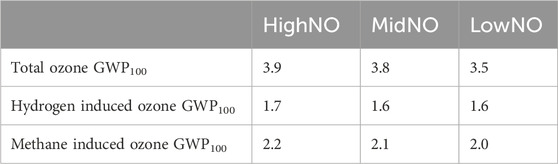
Table 3. Values for hydrogen GWP₁₀₀ due to changes in ozone in the hydrogen perturbation experiments in the HighNO, MidNO, and LowNO atmospheres. Row 2 is the total hydrogen GWP₁₀₀ due to ozone in the troposphere, row 3 is the component of the hydrogen GWP₁₀₀ due to ozone that derives directly from hydrogen and row 4 is the component that derives from the indirect methane component.

The perturbation in ozone scales slightly with anthropogenic NO_x levels. As NO_x levels increase, more ozone is present in the background atmosphere and the perturbation of both hydrogen and methane on this ozone is greater. A greater ozone perturbation leads to a higher radiative forcing from ozone and therefore a slightly larger hydrogen GWP₁₀₀ from ozone. The hydrogen GWP₁₀₀ due to ozone calculated for each atmospheric NO_x level is overall very similar.

3.3.3 Total tropospheric hydrogen global warming potential

The sum of the methane and ozone components of the hydrogen GWP represents a tropospheric GWP₁₀₀ for hydrogen. These component GWPs and the total tropospheric hydrogen GWPs calculated for the HighNO, MidNO, and LowNO atmospheres are shown in Figure 8. There is an additional stratospheric component of the hydrogen GWP₁₀₀ which is not estimated in these experiments. Warwick et al. (2023) calculated the tropospheric GWP₁₀₀ for hydrogen as 8.4 (under the conditions presented in IPCC AR6) and the total GWP₁₀₀ for hydrogen as 11.5 (with an uncertainty range of 6–18), indicating that the stratospheric component contributes to approximately a quarter to a third of the total GWP₁₀₀.

Figure 8

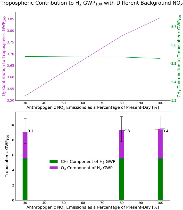
Figure 8. Top panel: The GWP₁₀₀ contribution in the troposphere from hydrogen acting on ozone (purple) and acting on methane (green) for the HighNO, MidNO, and LowNO levels of atmospheric NO_x (which are expressed here as % of present-day NO_x). Bottom panel: The contributions to the total tropospheric hydrogen GWP₁₀₀ in each atmosphere from hydrogen on methane (green) and on ozone (purple). The black bars on the panel indicate the upper and lower range of the total GWP₁₀₀ using the two end-member values for the global hydrogen deposition flux from Sand et al. (2023) (44 Tg a⁻¹and 73 Tg a⁻¹). The red and blue horizontal lines on the HighNO bar indicate the total tropospheric GWP₁₀₀ in the HighNO atmosphere in the climatological years before (red) and after (blue) the year analysed in detail in this study.

To estimate the uncertainty within these values, the calculation has been repeated with the range of global hydrogen deposition fluxes presented in Sand et al. (2023), which is 44–73 Tg a⁻¹. A 10% scaling to the deposition flux is applied in the hydrogen perturbed case. The range of tropospheric GWP in these cases is presented in Figure 8. The soil sink is highlighted in Sand et al. (2023) as the largest contributor to the uncertainty. The interannual variability of the tropospheric GWP can also be estimated by repeating the calculation for different model years. The model years following and prior to the year analysed here have been used. The meteorology will be different in these years according to sea surface temperatures and sea ice. For the previous year, the tropospheric GWP₁₀₀ for hydrogen in the HighNO experiment is 9.4, and the for the following year, the tropospheric GWP₁₀₀ is 9.5. These are also shown in Figure 8.

Overall, the total tropospheric GWP₁₀₀ for hydrogen in the HighNO atmosphere is 9.4, and in the LowNO atmosphere is 9.1. For the HighNO atmosphere, under the range of deposition fluxes presented in Sand et al., 2023, the tropospheric GWP₁₀₀ has a range of 7.8–11.2. Sand et al. (2023) calculated the hydrogen GWP from a multi-model ensemble and calculated a total atmospheric hydrogen GWP₁₀₀ of 11.6 ± 2.8 (given as one standard deviation). This includes the stratospheric component, for all models which were able to compute this.

Although we observe a very small trend of lower GWP₁₀₀ with lower atmospheric NO_x, this trend spans a large difference in atmospheric NO_x, and the range in our estimates is smaller than the multi-model range in Sand et al. (2023), indicating that in practical terms the GWP in each of our NO_x atmospheres is broadly constant. The conclusion from our work is therefore that, as atmospheric NO_x emissions decrease in the future, the impact of additional atmospheric hydrogen on global temperatures will vary relatively little. However, this finding may be complicated by changes in fluxes through relevant atmospheric reactions brought about by future changes in other pollutants such as VOCs and CO. These changes have not been explored within this study, as the simultaneous change of these species alongside NO_x has been investigated in previous literature (Schultz et al., 2003; Warwick et al., 2004; Jacobson, 2008; Warwick et al., 2023). This study has focused on impact of NO_x alone. The global warming potential of hydrogen demonstrates that some of the benefits which are associated with the switch from fossil fuels to renewable hydrogen will be offset by the atmospheric impact of any hydrogen which is leaked. This offset will depend on the leakage rate of hydrogen, which, at present, is very uncertain (Sand et al., 2023).

4 Conclusion

This study has shown that the global warming impact of hydrogen is intricately linked to atmospheric NO_x through key chemical reactions of ozone production and loss. Additional atmospheric hydrogen increases tropospheric ozone, most crucially through the additional HO₂ radicals that are produced when the hydrogen is oxidised by OH radicals. HO₂ converts NO to NO₂, the photolysis of which yields increased tropospheric ozone. As levels of atmospheric NO_x reduce in the future, as is expected with stricter emissions regulations and a greener energy mix, the chemistry of the ozone perturbation by hydrogen will change, leading to a slight reduction in the amount of ozone produced for the same amount of additional hydrogen. Overall, however, the total tropospheric hydrogen GWP₁₀₀ is simulated to change relatively little between substantially different levels of atmospheric NO_x (9.4 for 2010 anthropogenic surface NO_x emissions and 9.1 for 30% of these anthropogenic surface NO_x emissions). The current estimate for hydrogen GWP₁₀₀ can therefore be applied to future scenarios of differing NO_x, although this conclusion may be impacted by future changes in emissions of other reactive species.

Data availability statement

The raw data supporting the conclusions of this article will be made available by the authors, without undue reservation.

Author contributions

HB: Conceptualization, Data curation, Formal Analysis, Investigation, Methodology, Software, Validation, Visualization, Writing–original draft, Writing–review and editing. DS: Conceptualization, Funding acquisition, Methodology, Project administration, Resources, Supervision, Writing–review and editing. MH: Supervision, Writing–review and editing. NA: Methodology, Software, Writing–review and editing.

Funding

The author(s) declare that financial support was received for the research, authorship, and/or publication of this article. This study was funded by the HYDROGEN grant 320240 from the Norwegian Research Council and Energix, including a studentship for HB and by Researchfish 2024 - NE/X012735/1 - Topic A. Hydrogen Emissions: Constraining The Earth system Response (HECTER). Model simulations were run on the ARCHER2 UK National Supercomputing Service (https://www.archer2.ac.uk). This work used JASMIN, the UK collaborative data analysis facility.

Conflict of interest

The authors declare that the research was conducted in the absence of any commercial or financial relationships that could be construed as a potential conflict of interest.

The handling editor FP declared a past collaboration with the author HB.

Publisher’s note

All claims expressed in this article are solely those of the authors and do not necessarily represent those of their affiliated organizations, or those of the publisher, the editors and the reviewers. Any product that may be evaluated in this article, or claim that may be made by its manufacturer, is not guaranteed or endorsed by the publisher.

References

Archibald, A. T., O’Connor, F. M., Abraham, N. L., Archer-Nicholls, S., Chipperfield, M. P., Dalvi, M., et al. (2020). Description and evaluation of the UKCA stratosphere– troposphere chemistry scheme (strattrop vn 1.0) implemented in UKESM1. Geosci. Model Dev. 13, 1223–1266. doi:10.5194/gmd-13-1223-2020

CrossRef Full Text | Google Scholar

Crutzen, P. J. (1974). Photochemical reactions initiated by and influencing ozone in unpolluted tropospheric air. Tellus A Dyn. Meteorology Oceanogr. 26, 47–57. doi:10.3402/tellusa.v26i1-2.9736

CrossRef Full Text | Google Scholar

Ehhalt, D. H., and Rohrer, F. (2009). The tropospheric cycle of H₂: a critical review. Tellus B 61 (3), 500–535. doi:10.3402/tellusb.v61i3.16848

CrossRef Full Text | Google Scholar

Forster, P., Ramaswamy, V., Artaxo, P., Berntsen, T., Betts, R., Fahey, D. W., et al. (2007). “Changes in atmospheric constituents and in radiative forcing in: climate change 2007: the physical science basis,” in Contribution of working group I to the fourth assessment report of the intergovernmental panel on climate change. Editors S. Solomon, D. Qin, M. Manning, Z. Chen, M. Marquis, K. B. Averytet al. (Cambridge, United Kingdom and New York: Cambridge University Press).

Google Scholar

Gidden, M. J., Riahi, K., Smith, S. J., Fujimori, S., Luderer, G., Kriegler, E., et al. (2019). Global emissions pathways under different socioeconomic scenarios for use in CMIP6: a dataset of harmonized emissions trajectories through the end of the century. Geosci. Model Dev. 12, (4), 1443–1475. doi:10.5194/gmd-12-1443-2019

CrossRef Full Text | Google Scholar

Hoesly, R. M., Smith, S. J., Feng, L., Klimont, Z., Janssens-Maenhout, G., Pitkanen, T., et al. (2018). Historical (1750-2014) anthropogenic emissions of reactive gases and aerosols from the community emissions data system (CEDS). Geosci. Model Dev. 11, 369–408. doi:10.5194/gmd-11-369-2018

CrossRef Full Text | Google Scholar

Jacobson, M. Z. (2008). Effects of wind-powered hydrogen fuel cell vehicles on stratospheric ozone and global climate. Geophys. Res. Lett. 35, L19803. doi:10.1029/2008GL035102

CrossRef Full Text | Google Scholar

Lewis, A. (2021). Optimising air quality co-benefits in a hydrogen economy: a case for hydrogen-specific standards for NO_x emissions. Environ. Sci. Atmos. 1, 201–207. doi:10.1039/D1EA00037C

CrossRef Full Text | Google Scholar

Meinshausen, M., Vogel, E., Nauels, A., Lorbacher, K., Meinshausen, N., Etheridge, D. M., et al. (2017). Historical greenhouse gas concentrations for climate modelling (CMIP6). Geosci. Model Dev. 10, 2057–2116. doi:10.5194/gmd-10-2057-2017

CrossRef Full Text | Google Scholar

Naik, V., Voulgarakis, A., Fiore, A. M., Horowitz, L. W., Lamarque, J.-F., Lin, M., et al. (2013). Preindustrial to present-day changes in tropospheric hydroxyl radical and methane lifetime from the Atmospheric Chemistry and Climate Model Intercomparison Project (ACCMIP). Atmos. Chem. Phys. 13, 5277–5298. doi:10.5194/acp-13-5277-2013

CrossRef Full Text | Google Scholar

Patterson, J. D., Aydin, M., Crotwell, A. M., Pétron, G., Severinghaus, J. P., Krummel, P. B., et al. (2021). H₂ in antarctic firn air: atmospheric reconstructions and implications for anthropogenic emissions. Proc. Natl. Acad. Sci. 118, e2103335118. doi:10.1073/pnas.2103335118

PubMed Abstract | CrossRef Full Text | Google Scholar

Paulot, F., Pétron, G., Crotwell, A. M., and Bertagni, M. B. (2024). Reanalysis of NOAA H₂ observations: implications for the H₂ budget. Atmos. Chem. Phys. 24, 4217–4229. doi:10.5194/acp-24-4217-2024

CrossRef Full Text | Google Scholar

Rap, A., Richards, N. A., Forster, P. M., Monks, S. A., Arnold, S. R., and Chipperfield, M. P. (2015). Satellite constraint on the tropospheric ozone radiative effect. Geophys. Res. Lett. 42, 5074–5081. doi:10.1002/2015gl064037

CrossRef Full Text | Google Scholar

Riahi, K., van Vuuren, D. P., Kriegler, E., Edmonds, J., O’Neill, B. C., Fujimori, S., et al. (2017). The shared socioeconomic pathways and their energy, land use, and greenhouse gas emissions implications: an overview. Glob. Environ. Change 42, 153–168. doi:10.1016/j.gloenvcha.2016.05.009

CrossRef Full Text | Google Scholar

Sand, M., Skeie, R. B., Sandstad, M., Krishnan, S., Myhre, G., Bryant, H., et al. (2023). A multi-model assessment of the global warming potential of hydrogen. Commun. Earth Environ. 4, 203. doi:10.1038/s43247-023-00857-8

CrossRef Full Text | Google Scholar

Schultz, M. G., Diehl, T., Brasseur, G. P., and Zittel, W. (2003). Air pollution and climate-forcing impacts of a global hydrogen economy. Science 302, 624–627. doi:10.1126/science.1089527

PubMed Abstract | CrossRef Full Text | Google Scholar

Skeie, R. B., Myhre, G., Hodnebrog, Ø., et al. (2020). Historical total ozone radiative forcing derived from CMIP6 simulations. npj. Clim. Atmos. Sci. 3, 32. doi:10.1038/s41612-020-00131-0

CrossRef Full Text | Google Scholar

Stevenson, D. S., Young, P. J., Naik, V., Lamarque, J. F., Shindell, D. T., Voulgarakis, A., et al. (2013). Tropospheric ozone changes, radiative forcing and attribution to emissions in the atmospheric chemistry and climate model intercomparison project (ACCMIP). Atmos. Chem. Phys. 13, 3063–3085. doi:10.5194/acp-13-3063-2013

CrossRef Full Text | Google Scholar

van Marle, M. J. E., Kloster, S., Magi, B. I., Marlon, J. R., Daniau, A. L., Field, R. D., et al. (2017). Historic global biomass burning emissions for CMIP6 (BB4CMIP) based on merging satellite observations with proxies and fire models (1750-2015). Geosci. Model Dev. 10, 3329–3357. doi:10.5194/gmd-10-3329-2017

CrossRef Full Text | Google Scholar

Warwick, N. J., Archibald, A. T., Griffiths, P. T., Keeble, J., O’Connor, F. M., Pyle, J. A., et al. (2023). Atmospheric composition and climate impacts of a future hydrogen economy. Atmos. Chem. Phys. 23, 13451–13467. doi:10.5194/acp-23-13451-2023

CrossRef Full Text | Google Scholar

Warwick, N. J., Bekki, S., Nisbet, E. G., and Pyle, J. A. (2004). Impact of a hydrogen economy on the stratosphere and troposphere studied in a 2-d model. Geophysical Research Letters 31, L05107. doi:10.1029/2003GL019244

CrossRef Full Text | Google Scholar

Zheng, B., Chevallier, F., Yin, Y., Ciais, P., Fortems-Cheiney, A., Deeter, M. N., et al. (2019). Global atmospheric carbon monoxide budget 20002017 inferred from multi-species atmospheric inversions. Earth Syst. Sci. Data 11, 1411–1436. doi:10.5194/essd-11-1411-2019

CrossRef Full Text | Google Scholar