 Zhenning Huang
 Ning Sun2
- 1State Grid Shandong Electric Power Company, Shandong, Jinan, China
- 2State Grid Yantai Power Company, Shandong, Jinan, China
Multiple microgrids interconnect to form a microgrid cluster. To fully exploit the comprehensive benefits of the microgrid cluster, it is imperative to optimize dispatch based on the matching degree between the sources and loads of each microgrid. The power of distributed energy sources such as wind and photovoltaic systems and the sensitive loads in microgrids is related to the regional weather characteristics. Given the relatively small geographical scope of microgrid areas and the fact that distributed energy sources and loads within the grid share the same weather characteristics, simultaneous ultra-short-term forecasting of power for both sources and loads is essential in the same environmental context. Firstly, the introduction of the multi-variable uniform information coefficient (MV-UIC) is proposed for extracting the correlation between weather characteristics and the sequences of source and load power. Subsequently, the application of factor analysis (FA) is introduced to reduce the dimensionality of input feature variables. Drawing inspiration from the concept of combination forecasting models, a combined forecasting model based on Error Back Propagation Training (BP), Long Short-Term Memory (LSTM), and Bidirectional Long Short-Term Memory Neural Network (BiLSTM) is constructed. This model is established on the MV-UIC-FA foundation for the joint ultra-short-term forecasting of source and load power in microgrids. Simulation is conducted using the DTU 7K 47-bus system as an example to analyze the accuracy, applicability, and effectiveness of the proposed joint forecasting method for sources and loads.
1 Introduction
In microgrids, there exists a substantial presence of distributed generation (DG) sources such as wind and photovoltaic, along with actively time-varying sensitive loads. The power output of DG and load power are both influenced by complex factors such as regional weather, date, and special events (Zhu et al., 2023). As microgrid deployment and utilization expand, neighboring microgrids interconnect to form coexistence of distributed generation and loads in the same environment, it is imperative to simultaneously conduct joint prediction of source and load power under the same weather characteristics (Yu et al., 2024). To fully exploit the comprehensive benefits of microgrid clusters, it is necessary to coordinate and optimize the operation within each microgrid cluster and between microgrid clusters and distribution networks based on the matching degree of sources and loads in each microgrid. Ultra-short-term prediction of source and load power serves as the foundation for this endeavor. Given the relatively small geographical area where microgrids are located and the coexistence of distributed generation and loads in the same environment, it is imperative to simultaneously conduct joint prediction of source and load power under the same weather characteristics (Wang et al., 2024).
Microgrid source and load power ultra-short-term prediction methods encompass mathematical statistical approaches (Safari et al., 2018) and artificial intelligence methods (Zhu et al., 2023). Artificial intelligence methods excel in capturing the nonlinear relationship between inputs and outputs, demonstrating robust data analysis and forecasting capabilities. They have emerged as pivotal techniques for ultra-short-term prediction of microgrid source and load power (Zhang et al., 2024). Internationally recognized experts and scholars, considering factors such as meteorological and calendar features, have employed various single prediction models like Error Back Propagation Training (BP), deep recurrent neural network (DRNN), and Long Short-Term Memory (LSTM) to forecast short-term power for microgrid DG and loads. In response to the escalating electricity demand and restructuring of power systems, researchers have proposed a long-term electricity demand forecasting method based on BP (Masoumi et al., 2020). This approach utilizes a Time Series Neural Network (TSNN) structure, employing forward propagation of input load data, error computation, and weight updating through backpropagation in training steps, thereby achieving self-learning and self-organization. To enhance photovoltaic (PV) generation prediction accuracy, researchers have developed a forecasting algorithm based on LSTM (Hossain and Mahmood, 2020). This algorithm combines synthesized weather forecasts with historical solar radiation data and publicly available sky type predictions for the host city, utilizing the K-means algorithm for dynamic sky type classification. This approach significantly improves prediction accuracy, achieving an increase in accuracy ranging from 33% to 44.6% compared to predictions using fixed sky types. In another study, G. W. Chang and H.J. Lu integrated grey data preprocessors with DRNN for day-ahead output prediction in photovoltaic generation (Chang and Lu, 2018). However, due to the distinct advantages of different prediction models, achieving optimal predictive performance with a single model often proves challenging (Zhu et al., 2019). To address this, experts and scholars adopt a “modal decomposition-combined prediction” approach: firstly, utilizing modal decomposition methods to break down historical data of sources and loads into components with different frequencies, thereby reducing the complexity of input data; secondly, introducing a combined model approach, selecting prediction models with varying performances for different frequency modal components, and ultimately obtaining the final prediction results through summation and reconstruction. For instance, adaptive noise-aided complete ensemble empirical mode decomposition with adaptive noise (CEEMDAN) was employed to decompose the raw data of building sub-item energy generation (Lin, 2022). Subsequently, predictions for different modal components were conducted using BiLSTM. The final photovoltaic power generation was obtained through summation and reconstruction. Another study combined three models, optimized extreme learning machine (ELM), backpropagation neural network (BPNN), and dynamic recursive neural network (ELMAN), for short-term forecasting of wind power plant output (Ma et al., 2023). In a separate study, variational mode decomposition (VMD) was utilized to decompose load raw data into different frequency modal components (Yue et al., 2023). Subsequently, a Bagging ensemble ultra-short-term multivariate load forecasting method was developed based on gated recurrent unit (GRU), LSTM, and BiLSTM models, leading to enhanced prediction accuracy. In the field of microgrid power forecasting, predictions of source power and load power are typically conducted independently based on their respective environmental factors. However, this approach may overlook an important reality: under the same environmental conditions, weather characteristics may simultaneously affect both the source side (such as photovoltaic and wind power) and the load side of the microgrid. For instance, sunny weather may increase the output of photovoltaic generation while also raising the electricity demand for cooling devices like air conditioners. Therefore, decoupling the predictions of source power and load power may lead to reduced accuracy in forecasting results, impacting the economic dispatch and stable operation of the microgrid. Currently, research on how to comprehensively consider the simultaneous impact of weather characteristics on both the source and load sides of microgrids is relatively limited. Most existing models focus on predicting power for a single energy source type or only consider the influence of weather factors on load demand. Such independently predictive methods may fail to fully capture the comprehensive effects of weather changes on the overall performance of microgrids. To enhance the accuracy and reliability of microgrid power forecasting, future research needs to develop more comprehensive models that can simultaneously consider the generation characteristics of multiple energy sources and the response of load demand to weather changes.
To predict both the source and load power in a microgrid under the same weather conditions simultaneously, it is necessary to analyze the concurrent correlation between the two variables and the weather features. Extracting weather characteristics that have a significant impact on the source and load power in the microgrid enhances predictive capability. Common methods for feature extraction include the Pearson coefficient (Xu et al., 2023), Spearman coefficient (Qun et al., 2023), Maximum Information Coefficient (MIC) (Reshef et al., 2011), and Uniform Information Coefficient (UIC) (Jiang et al., 2023). Reference Jiang et al. (2023) utilized the Uniform Information Coefficient (UIC) to analyze the correlation between weather characteristics and load power. Compared to the other three algorithms, UIC is specifically designed for analyzing relationships among multidimensional variables, making it more suitable for handling complex meteorological data and load power data, which are often multidimensional. Moreover, it is computationally more efficient. It achieves this by employing a simplified technique based on uniformly partitioned data grids, replacing the dynamic programming steps in MIC computation, thus reducing computational costs. The aforementioned approaches focus solely on extracting the correlation between a single dependent variable (e.g., DG output or load power) and a single independent variable (weather feature), thereby unable to capture the correlation between multiple dependent variables (DG output and load power) and a single independent variable (weather feature). Addressing this limitation, this study investigates the simultaneous correlation between source and load power in a microgrid and weather features, conducting research on the joint ultra-short-term prediction of source and load power in a microgrid. Additionally, commonly used dimensionality reduction algorithms include Principal Component Analysis (PCA) (Wang et al., 2023), Independent Component Analysis (ICA) (Kobayashi and Iwai, 2018), Factor Analysis (FA) (Ramirez et al., 2019; Wu et al., 2024), etc. FA merges numerous features into several representative common factors to extract latent factors among features, accurately capturing the relevant information in the data (Zhou et al., 2020). FA is particularly effective in capturing the underlying structure of data by reducing the dimensionality and identifying the shared variance among variables. It helps uncover the latent factors that explain the correlations and patterns within the dataset, facilitating a deeper understanding of the relationships among the features.
In conclusion, this manuscript contemplates the impact of weather features in the region of a microgrid on DG and load power simultaneously. A joint ultra-short-term prediction model for source and load power in a microgrid is proposed. Initially, the concept of the Multi-Variable Uniform Information Coefficient (MV-UIC) is introduced to analyze and compute the correlation coefficients between weather features and the sequences of microgrid source and load power, facilitating the elimination of redundant features. To diminish the dimensionality of input features for the prediction models of source and load power, FA is employed. Addressing the pronounced nonlinearity and non-stationarity in microgrid source and load power, a model is established by amalgamating BP, LSTM, and BiLSTM models, considering the correlation between weather features and multiple variables. Using the DTU 7K 47-bus as an example in a real system (Baviskar et al., 2021), specifically with 3 wind farms serving as DG and an aggregated load, the proposed prediction model is pre-trained using historical data from the power grid dataset. The accuracy, applicability, and effectiveness of the proposed joint prediction method for source and load are then analyzed in the DTU 7K 47-bus system.
2 A weather feature extraction method based on MV-UIC
The Uniform Information Coefficient (UIC) algorithm, pioneered by Mousavi and Baranuk (2022), introduces an innovative methodology for feature extraction. UIC facilitates the analysis of the correlation between two univariate variables, making it particularly well-suited for addressing feature extraction challenges in large-scale datasets. Let A = [a1, …, an] and B = [b1, …, bn] denote two sets of feature vectors with a sequence length of n. The model for the UIC is shown in Eq. 1.
where IUIC(A; B) represents the Uniform Information Coefficient between A and B; I (A; B) denotes the Mutual Information Coefficient between A and B; r and s correspondingly indicate the segmentation numbers for A and B; min{r, s} represents the minimum value between r and s.
In order to ascertain the simultaneous correlation of the dependent variables, source and load power, with weather characteristics in a microgrid, this paper adopts an extension of the method presented in Wang (2020) and Ng et al. (2023), which expands from the maximum information coefficient between two variables to the multivariate case. The UIC for the two variables is extended, introducing the Multi-variable Uniform Information Coefficient (MV-UIC) algorithm. The specific definition is outlined as follows: The dataset D consists of three variables: (PDG, PL), and H. H represents the independent variable, denoting the regional weather feature vector, while (PDG, PL) signify the source and load power vectors, respectively, in a microgrid. H is allocated to the x-axis as X = [xi], where “n” denotes the sequence length. Similarly, (PDG, PL) are allocated to the y-axis as Y = [yi]. H is uniformly divided into r blocks, and (PDG, PL) into s blocks. After partitioning dataset D, r × s grids are obtained, with each grid representing a subset of data points. The ratio of the number of points falling into corresponding grid to the total number of points defines the approximate probability density of that grid. Subsequently, the mutual information coefficient between the weather feature variable H and (PDG, PL) is derived. Normalization is then performed to obtain the multivariate unified information coefficient between the two variables PDG, PL, and the univariate H in dataset D. The steps for obtaining MV-UIC are as follows:
(1) For a given three-variable dataset D and positive integers r, s, where r, s ≥ 2, D = {(PDG, PL), H}, the mutual information between them, denoted as IMI(D, r, s, (PDG, PL); H):
where p(x) represents the edge probability density of the regional weather characteristic variable H uniformly divided into r grids, p(y) represents the edge probability density of the source and load power vectors (PDG, PL) uniformly divided into s grids, and p (xy) represents the joint probability density of the dataset D divided into r×s grids.
According to the uniform division method, the length of each segment after evenly dividing the x and y axes into r and s is:
where dx and dy represent the lengths of partition units for X and Y, respectively;
(2) The formula for calculating the MV-UIC between the regional weather feature vector H and the source and load power vectors (PDG, PL) in a microgrid is as follows:
where I (D, r, s, (PDG, PL), H) denotes the mutual information among the three entities; log2 (min{r, s}) represents normalization, with min{r, s} being the minimum value between r and s, and
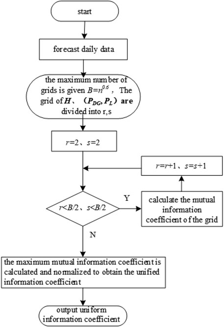
Figure 1. Flow chart of the MV-UIC algorithm.
Based on Eqs 2–4, the MV-UIC between microgrid source, load power, and weather features can be computed. A higher value indicates a stronger correlation between the respective weather feature and the source/load power. Selecting weather features with high correlations as inputs for source/load power prediction models helps filter out remaining features, thereby mitigating issues related to excessive variables and redundant computations.
3 Inputfeature dimensionality reduction based on FA
Due to the strong interrelationships among weather feature variables, regression analysis encounters a certain degree of collinearity issue. FA serves as a multivariate statistical method that, by solving the correlation matrix of variables, identifies common factors describing relationships among numerous variables and simplifies data, thereby reducing the dimensionality of the dataset. The fundamental principles and computational procedures of FA are detailed in Wu et al. (2024), wherein the basic model entails the linear relationship between observed variables and common factors as Eq. 5:
In the equation, Ψ represents the matrix of observed variables; F stands for the matrix of common factors; ι denotes the factor loading matrix, illustrating the relationship between each observed variable and the common factors; E signifies the matrix of factor variances.
Utilizing the MV-UIC obtained in Section 1, weather feature variables with similar attributes are grouped together and represented by a common factor. Analyzing the correlation between variables involves solving the eigenvalues and corresponding orthogonal eigenvectors of the correlation matrix. Based on the eigenvalues of the correlation matrix, the variance contribution rate and cumulative contribution rate of common factors are computed, with a cumulative contribution rate exceeding 85% serving as the criterion for determining the number of common factors. Subsequently, factor matrix rotation yields the factor loading matrix. Factor scores are then calculated using regression analysis. Higher values in the factor score matrix indicate a more significant representation of the feature by the respective factor in the dataset. Dimensionality reduction of input features for source/load power prediction is conducted based on factor scores.
4 A short term joint prediction model for microgrid source and load power considering weather characteristics and multivariable correlation
In microgrid systems, predicting source and load power is crucial for stable operation. Due to their nonlinearity and non-stationarity, single models struggle to capture these complexities, leading to poor performance. Empirical Mode Decomposition (EMD) decomposes source-load sequences into Intrinsic Mode Functions (IMFs), enhancing prediction accuracy by describing variations and periodicities. To improve predictive performance further, joint prediction methods integrate multiple models’ advantages. Weighting different models appropriately creates a comprehensive model considering various characteristics and IMFs, yielding more accurate results. Additionally, predicting source and load power under similar weather conditions requires analyzing their correlation with weather features. Traditional methods fail to capture this correlation simultaneously, unlike the Multi-variable Uniform Information Coefficient (MV-UIC), which evaluates it effectively. MV-UIC’s application enables feasible joint prediction of source and load, quantifying the correlation between multiple dependent variables and a single independent variable, aiding in constructing precise prediction models.
4.1 BP network
The BP network is a multi-layer feedforward neural network. The topology of a three-layer BP network is illustrated in Figure 2, encompassing an input layer, an output layer, and a single hidden layer. Each neuron is connected to all neurons in the subsequent layer, with no interconnections among neurons within the same layer.
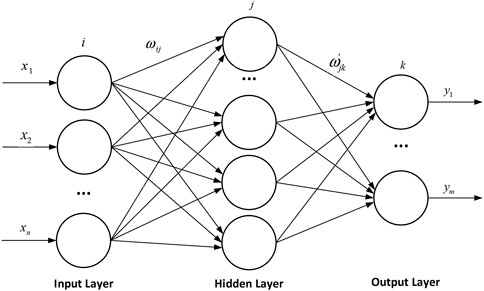
Figure 2. BP network with three layers.
The BP network minimizes error using gradient descent. Standard BP lacks momentum consideration, causing slow convergence. Enhanced BP integrates momentum to reduce oscillations and hasten convergence. The objective function is defined accordingly. The objective function is defined as Eq. 6:
where
4.2 LSTM
The LSTM represents an enhanced version of the Recurrent Neural Network (RNN). Introduced and subsequently refined with additional forget gates, the improved LSTM addresses the issue of “vanishing gradients” encountered during model training. Capable of learning both short-term and long-term dependencies in time series data, it stands as one of the most successful RNN architectures, finding applications across various domains. The fundamental unit of an LSTM network, as depicted in Figure 3.
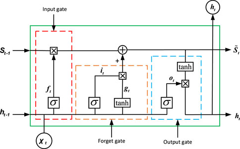
Figure 3. Basic unit of LSTM network.
The fundamental unit of an LSTM network comprises forget gates, input gates, and output gates. The forget gate determines the extent of memory to be retained from the state cell, influenced by the input χt, previous state
where
4.3 BiLSTM
The BiLSTM is an advanced enhancement of the conventional unidirectional LSTM, integrating both a forward LSTM layer and a backward LSTM layer, each influencing the output. While the unidirectional LSTM adeptly utilizes historical data to mitigate long-distance dependency issues, the BiLSTM benefits from the incorporation of both forward and backward sequence information, thoroughly considering past and future data to significantly enhance model prediction accuracy. The architecture of the BiLSTM, as illustrated in Figure 4.
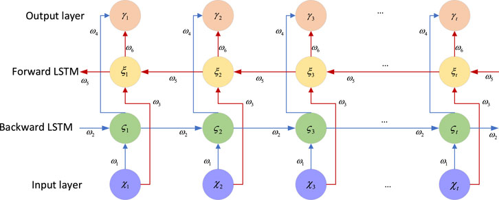
Figure 4. Structure of BiLSTM network.
The architecture of the BiLSTM involves updates to the hidden layers of the forward LSTM, the backward LSTM, and the process leading to the final output of the BiLSTM, delineated in Eqs 13–15:
where
4.4 VMD
The specific steps of the VMD algorithm are described as follows:
(1) Define the variational problem: In order to decompose the given original sequence
where the original sequence
(2) The formula for the Lagrangian transformation is shown in Eq. 17: In order to solve the optimal solution problem of the above variational constraint, Lagrange multiplier
(3) Alternate update: initialize
where ψ is the number of iterations;
(4) Submode output as Eq. 19: according to Eq. 18 determine whether the termination conditions, if not, return to step 3), if satisfied, the Fourier inverse transformation of the last update
where
4.5 Model construction
The paper exemplifies a 15-min interval to predict the microgrid’s source and load power sequences for the next hour. Due to the long time resolution and insufficient accuracy of numerical weather forecasts, only historical meteorological data is utilized as weather feature input during the selection of input features for the prediction model. This data is combined with historical sequences of microgrid source and load power to collectively form the input matrix. Regarding historical features, five historical similar days with significant correlation to the current weather and the historical power measurement values from the past 5 days are specifically chosen as historical data (Wang, 2020).
The source and load power in microgrids exhibit strong nonlinearity and non-stationarity characteristics, rendering single predictive model methods limited in both fitting performance and prediction accuracy. To enhance power prediction accuracy, this study drew upon the methods outlined in Yue et al. (2023). Initially, VMD was employed to decompose historical source and load power time series under different weather conditions, yielding multiple IMF components of various frequencies. Subsequently, the permutation entropy (PE) values of each IMF were computed, and based on these PE values, low, medium, and high-frequency input matrices were constructed. Considering the concurrent temporal correlation of current microgrid source and load power values with past and future time information, three homogeneous recursive neural network models—BP, LSTM, and BiLSTM—were selected for their robust handling of time-series data. These models were employed as base learners, utilizing a bootstrapping method to acquire diverse training set samples, which were then used to train the base learners. This approach enabled the prediction of different frequency components, which were subsequently combined to obtain microgrid source and load power forecasts. High-frequency data changes typically exhibit strong sequential dependencies and long-term trends. LSTM models excel at capturing long-term dependencies within sequential memory and adaptively adjusting the complexity and variability of sequence patterns, making them suitable for predicting high-frequency data trends. Medium-frequency data is often influenced by preceding and succeeding time-step data, exhibiting certain contextual dependencies. BiLSTM models, equipped with both forward and backward memory units, can simultaneously process forward and reverse sequence information, thus better capturing contextual relationships within medium-frequency data and enhancing prediction accuracy. Low-frequency component variations are relatively slow and stable. The training process of BP neural networks is relatively straightforward, capable of providing forecasts of future trends by learning the input-output mapping relationships of historical data.
In consideration of the aforementioned, this paper contemplates the correlation between weather characteristics and multivariable factors, proposing a joint prediction model for microgrid source and load power based on MV-UIC-FA. The schematic diagram of the prediction model is illustrated in Figure 5. The specific prediction steps are as follows:
(1) Acquiring meteorological characteristics for the forecasted day involves retrieving weather information strongly correlated with source and load power from historical daily datasets. Similar days are selected to construct datasets under distinct weather types.
(2) Data completion: To address gaps in the source and load datasets, missing values are replenished with the average of six data points before and after the sampling point.
(3) Normalization: Employing the Z-score algorithm for normalization ensures a balanced distribution of data.
(4) Timestamp alignment: Concerning the alignment of timestamps in the dataset, this study will utilize spline interpolation for the alignment operation.
(5) Feature selection: Utilizing MV-UIC, an analysis is conducted on the correlation between weather characteristics and microgrid source/load sequences to filter out weather features closely associated with the prediction task.
(6) Feature dimensionality reduction: Employing the FA method, the selected weather feature sequences are subjected to dimensionality reduction while preserving the fundamental information of the original features.
(7) Offline model training: Constructing input matrices for the prediction model involves integrating the processed features with source and load sequences. Following the training methodology of the combined prediction model, the processed dataset is partitioned into training, validation, and testing sets in a ratio of 7:2:1. Subsequently, offline training is conducted to derive the prediction model.
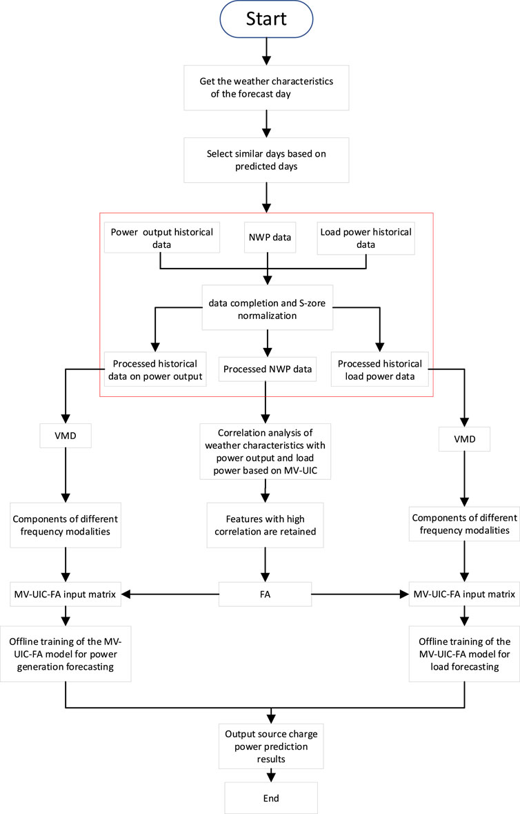
Figure 5. Joint prediction model of microgrid source and load power based on MV-UIC-FA.
5 Example analysis
To substantiate the rationality of the jointly proposed ultra-short-term forecasting methodology for microgrid source and load power, it is imperative to concurrently acquire the original data pertaining to weather characteristics, distributed power sources, and load power within the microgrid’s geographical domain. The source, load, and weather feature data for the DTU 7K 47-bus system (Baviskar et al., 2021), available on the official website, are comprehensive for the period spanning from 1 January 2015, to 31 August 2015. Accordingly, the simulation testing in this study is conducted utilizing the data from this specific timeframe.
The DTU 7K 47-bus system is an open-source multi-voltage level distribution grid model developed by the Technical University of Denmark (DTU). Named the DTU 7k-Bus Active Distribution Grid Model, it spans three voltage levels and is geographically modeled for network topology. Key features include multi-voltage levels enabling analysis of challenges and opportunities in renewable energy-dependent grids, geographical data-based network topology modeling for real-world grid operation simulation, simulation data derived from weather and measured data, and open accessibility for research and educational purposes. Data primarily sourced from DTU’s official data-sharing platform, DTU Orbit, allows researchers access for power system analysis, renewable energy integration studies, grid planning, and operational simulations.
The DTU 7K 47-bus system, depicted in Supplementary Appendix Figure S2, is interconnected with the external grid via the B-0 transformer at the B-9 bus; the system encompasses three wind farms, composed of fourth-generation controllable wind turbines with installed capacities of 12, 15, and 15 MW, respectively. Due to the location of the DTU 7K 47-bus testing system within the Danish territory, meteorological data is sourced from the Danish Meteorological Institute. The selected weather features include reflectance, snow reflectance, high cloud cover, low cloud cover, 2-m relative humidity, snow density, 2-m specific humidity, 10-m wind speed, 30-m wind speed, 50-m wind speed, 70-m wind speed, 100-m wind speed, atmospheric pressure, 2-m temperature, total cloud cover, visibility, 10-m wind direction, and mid-level cloud cover, totaling 18 variables. The sampling, normalization, and offline training data sample quantities for source and load data remain consistent. The sampling frequency is 15 min, resulting in a total of 23,328 samples. Z-score algorithm is employed for normalization. Subsequently, 16,330 samples are randomly chosen for training, 4,665 for validation, and 2,333 for testing. The input time series length is set at 96.
The models in this study are trained using the Python software. The performance of the proposed methodology is assessed through the utilization of root mean squared error (RMSE) and mean absolute error (MAE) they are as Eqs 20, 21:
In the equation: v is the true value of the source load;
5.1 Simulation case 1: testing of weather feature extraction and dimensionality reduction methods
5.1.1 Feature extraction and factor analysis based on MV-UIC for dimensionality reduction
To substantiate the rationality of the proposed feature extraction algorithm across diverse seasons, this paper opts for the dates of April 30th (spring), June 30th (summer), August 31st (autumn), and February 28th (winter) as prediction days, aligning with the climatic nuances of Denmark. Historical days with correlation coefficients exceeding 0.8 concerning the prediction days are designated as analogous days. The input feature sequences encompass five historical source-load data points with a kin weather conditions, the source-load data from the past 5 days, and eighteen weather attributes. Four forecasted days’ weather features, along with the MV-UIC of source and load power, are extracted as delineated in Table 1.
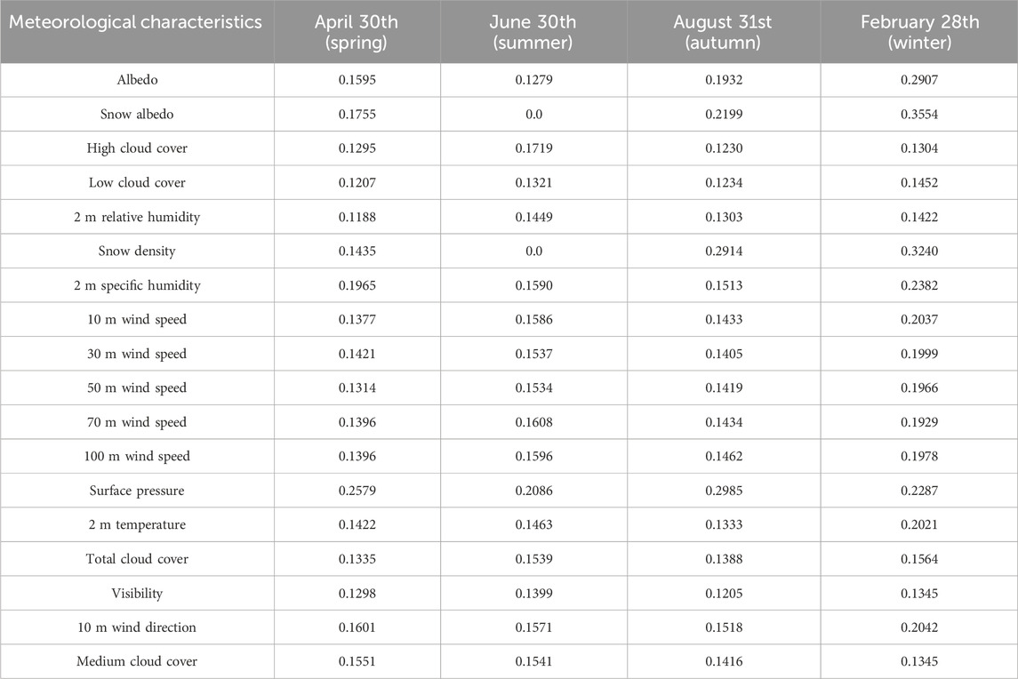
Table 1. Weather characteristics and MV-UIC of source and load power for four forecast days.
From Table 1, it can be observed that the weather characteristics vary across different seasons, exhibiting disparate MV-UICs concerning microgrid source and load power. These weather features manifest distinct correlations with source and load power. Given Denmark’s temperate maritime climate, precipitation (snow) and strong winds are predominantly observed during the autumn and winter seasons, occasionally culminating in extreme weather phenomena such as blizzards. Consequently, during the winter season, the information coefficients between snow density, wind speed, and source and load power stand at 0.324 and 0.2037, respectively, indicating considerable magnitudes. These findings align with Denmark’s actual climatic conditions and geographical location, thereby corroborating the rationality and efficacy of the proposed MV-UIC feature extraction method.
5.1.2 Using FA to reduce the dimension of input features
The FA method is employed herein to capture the common factors among input features by constructing a factor score matrix, facilitating dimensionality reduction for the 18 input features across four forecast days. The total variance explanation table for the spring is presented in Table 2, while the factor score matrix is shown in Table 3. The variance explanation tables and factor score matrices for the other three forecast days can be found in Supplementary Appendix SA. From the variance analysis in Table 2, it is evident that six common factors are extracted from the input features in this study. As indicated by the factor score matrix in Table 3, these factors are the wind speed factor, 2 m information factor (including 2 m relative humidity, 2 m specific humidity, and 2 m temperature), albedo factor, cloud cover factor, surface pressure factor, and wind direction factor. The cumulative variance contribution rate of these common factors is 97.966% (>85%), suggesting that these six common factors encompass the majority of the effective information within the sequences of 18 key input features. This is of significant importance for interpreting the variations in the original data.
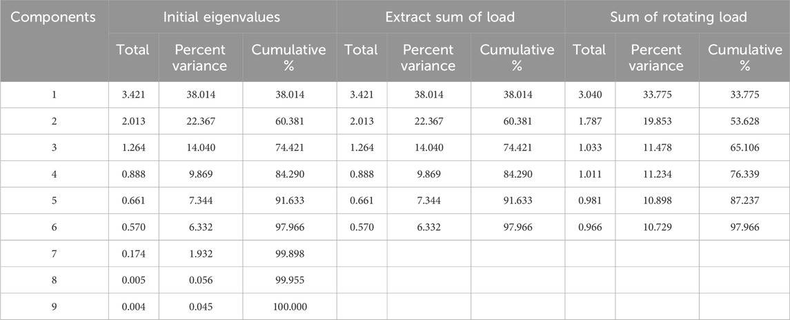
Table 2. Total variance interpretation table.
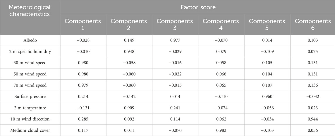
Table 3. Factor score matrix.
5.1.3 Test of feature extraction and factor-based dimensionality reduction method based on MV-UIC
To mitigate the non-stationarity of microgrid sources and loads, an initial step involves employing VMD to decompose the time series of source and load data for similar and forecast days. The VMD decomposition results are presented in Supplementary Appendix SB. This process yields various modal sub-sequences of source and load power. Subsequently, the PE values are computed for each sub-sequence. Sequences with PE values exceeding 0.55 are designated as high-frequency sequences, those with PE values ranging from 0.25 to 0.55 are categorized as mid-frequency sequences, and sequences with PE values below 0.25 are identified as low-frequency sequences. The decomposition results of the spring forecast day source and load power are illustrated in Supplementary Appendix Figure SFA1, revealing the absence of low-frequency components in the wind power output sequence.
In order to validate the rationality of the proposed feature extraction algorithm in different seasons, the study utilized the all feature (AF) of the forecast day and input features extracted based on MV-UIC-FA separately as inputs for the prediction model. Three types of base learners—BP, LSTM, and BiLSTM—were employed to individually predict the low, mid, and high-frequency components of source and load power. The corresponding evaluation metrics for the prediction results are presented in Table 4, with a prediction step of 4 for all control groups. Upon examination of Table 4, it is observed that compared to using all weather features as input for the prediction model, employing MV-UIC to extract and dimensionally reduce weather features before prediction resulted in a reduction of 13.46% and 17.85% in RMSE and MAE for electric power prediction, respectively. For load power prediction, the RMSE and MAE were reduced by 17.62% and 17.31%, respectively. This indicates a significant improvement in prediction accuracy, validating the effectiveness of the proposed approach across different seasons.

Table 4. Evaluation indexes of source and load power prediction models after dimensionality reduction of AF and MV-UIC-FA.
This simulation yielded the corresponding predictions as shown in Figures 6, 7.
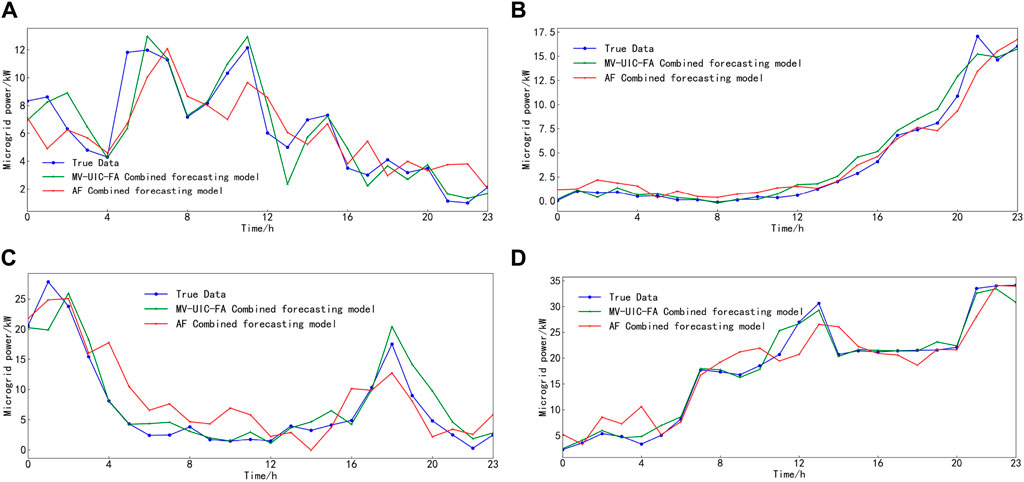
Figure 6. Microgrid power prediction results for four prediction days. (A) Spring. (B) Summer. (C) Fall. (D) Winter.
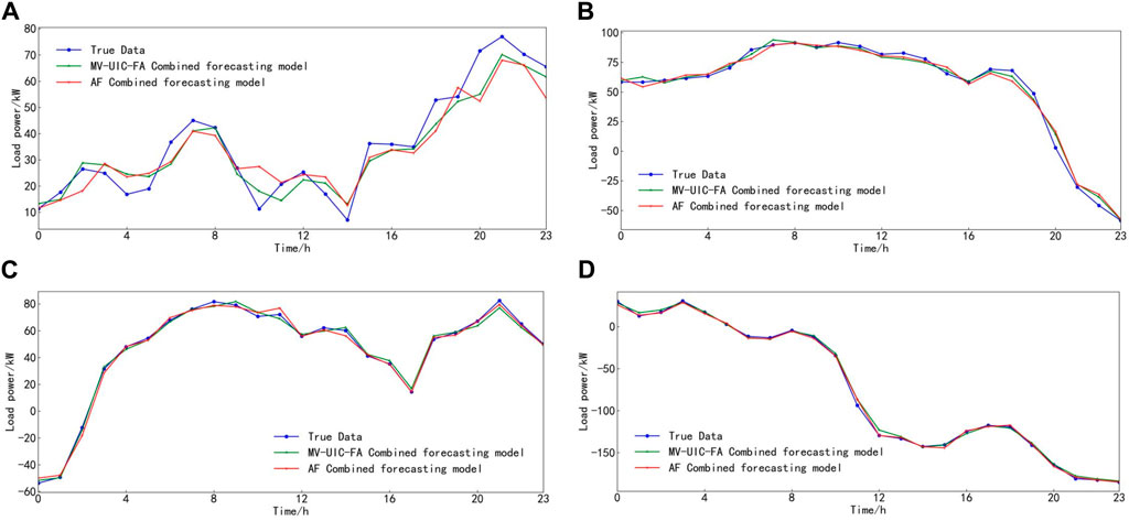
Figure 7. Microgrid load prediction results for four prediction days. (A) Spring. (B) Summer. (C) Fall. (D) Winter.
5.2 Simulation case 2: comparative testing of accuracy of different prediction models
To verify the accuracy of the joint prediction model for microgrid source and load power based on MV-UIC-FA proposed in this paper, predictions of source and load power for four forecasting days were initially conducted using the MV-UIC-FA prediction model. Subsequently, comparisons were made with the results of three single prediction models, namely BP (MV-UIC-BP, MV-B), LSTM (MV-UIC-LSTM, MV-L), and BiLSTM (MV-UIC-BiLSTM, MV-Bi). These models utilized dimensionally reduced input features. Evaluation metrics such as RMSE and MAE for the corresponding prediction results were obtained and are presented in Table 5 (with a prediction step of 4 for all control groups). Additionally, comparisons between the predicted results for source and load power for the four forecasting days and the actual data are illustrated in Figures 8, 9.
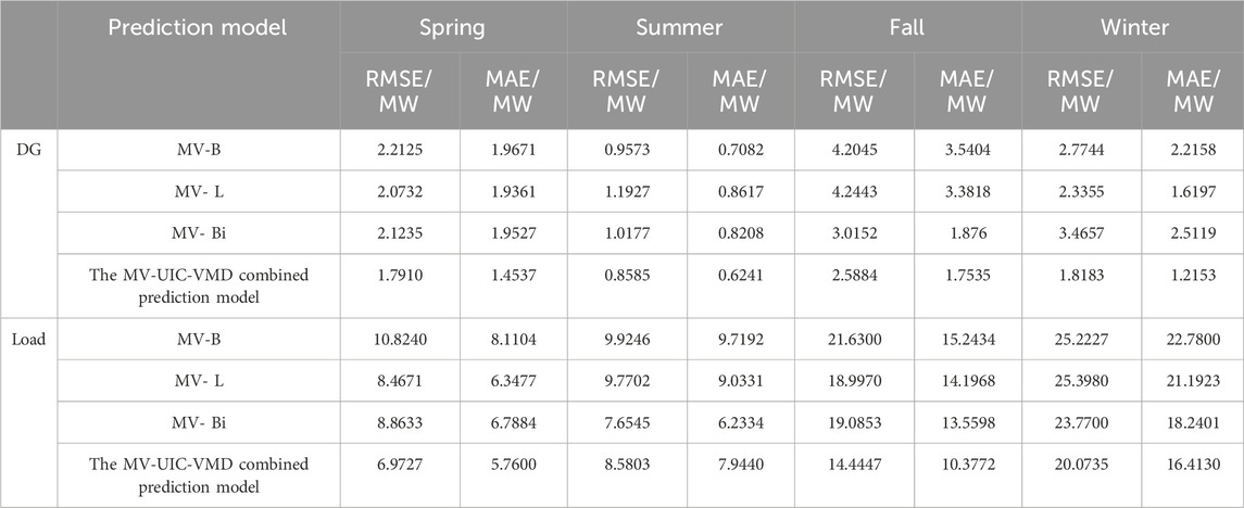
Table 5. Evaluation indexes of RMSE and MAE for different prediction models.
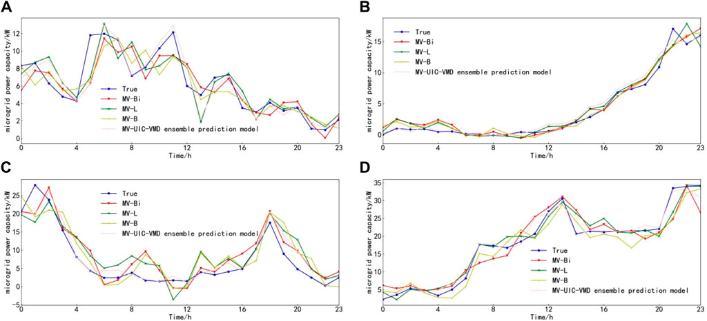
Figure 8. Microgrid power prediction results for four prediction days. (A) Spring. (B) Summer. (C) Fall. (D) Winter.
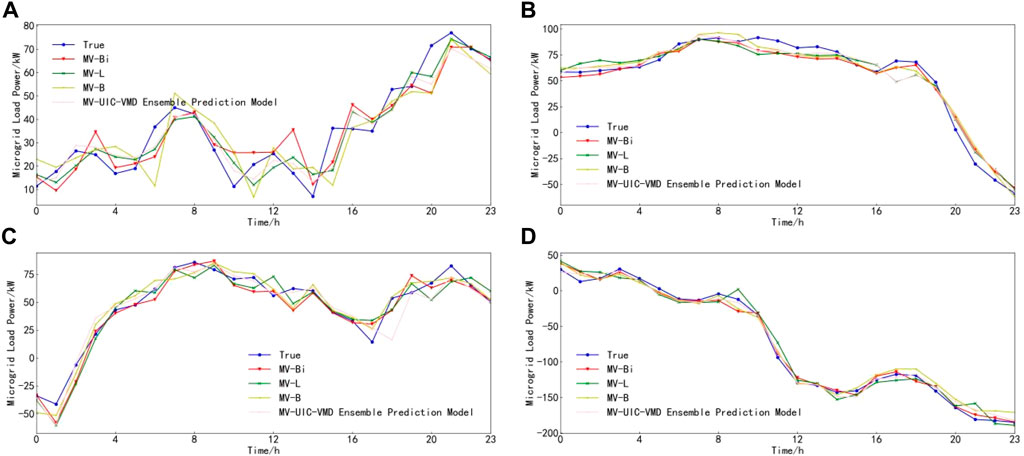
Figure 9. Microgrid load prediction results for four prediction days. (A) Spring. (B) Summer. (C) Fall. (D) Winter.
From Figures 8, 9, it can be observed that among the predicted power for the four forecasting days, the results of the three individual forecasting models are similar, while the combined forecasting model fully exploits the advantages of each individual forecasting model, yielding superior forecasting results. As seen from Table 5, the proposed models in this study outperform various baseline models in terms of their RMSE and MAE. Specifically, compared to the forecasting results of the BP, LSTM, and BiLSTM models, the employment of the proposed model in this study reduces the RMSE and MAE of the power supply by 25.57%, 25.71%, 23.48%, and 33.4%, 31.41%, 26.92%, respectively, and reduces the RMSE and MAE of the load power by 25.69%, 18.69%, 18.33%, and 26.79%, 17.71%, 19.07%, respectively.
5.3 Simulation case 3: comparative testing of accuracy of different prediction models
In this section, the accuracy and robustness of the proposed joint prediction model for microgrid source and load power based on MV-UIC-FA are validated using the IEEE 118-bus standard distribution network test system (Youssef et al., 2020) as shown in Figure 10. Actual power and load data from the 2014 Global Energy Forecasting Competition (GEFC) (Hong et al., 2016) are utilized as the training and testing datasets. Controllable wind turbines of the fourth generation, each with a rated capacity of 1 MW, are connected to buses 14, 25, 46, 49, 66, and 69 of the IEEE 118- bus test system. Load data and environmental weather characteristic data from the 2014 GEFC are extracted, covering the period from March 1st to 12th, 2005, with a sampling frequency of 1 h, totaling 288 h of data. This dataset is used for experimental simulations. Meteorological data utilized in the simulations are sourced from the publicly available local weather information on the website of the National Renewable Energy Laboratory (NREL) (NREL, 2024) in the United States. The dataset includes load and power sequences, temperature, weather type 1, humidity, visibility, weather type 2, perceived temperature, pressure, wind speed, cloud cover, wind resistance, precipitation intensity, dew point, and precipitation probability. Normalization is applied to both power and load data to meet simulation requirements. Missing values in the dataset are filled, and normalization is performed. The training and prediction datasets are divided in an 8:2 ratio. March 12th is selected as the prediction day.
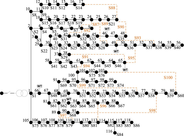
Figure 10. IEEE 118-bus standard power distribution system.
Based on the findings presented in Figure 11 and Table 6, it is evident that the predictive performance of the method proposed in this paper for forecasting source and load power within the IEEE 118-bus standard distribution network surpasses that of alternative individual methods, demonstrating superior predictive accuracy and commendable generalization capabilities.
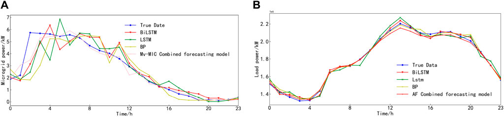
Figure 11. Results diagram of source and load power prediction of IEEE 118-bus standard distribution system. (A) DG. (B) Loads.
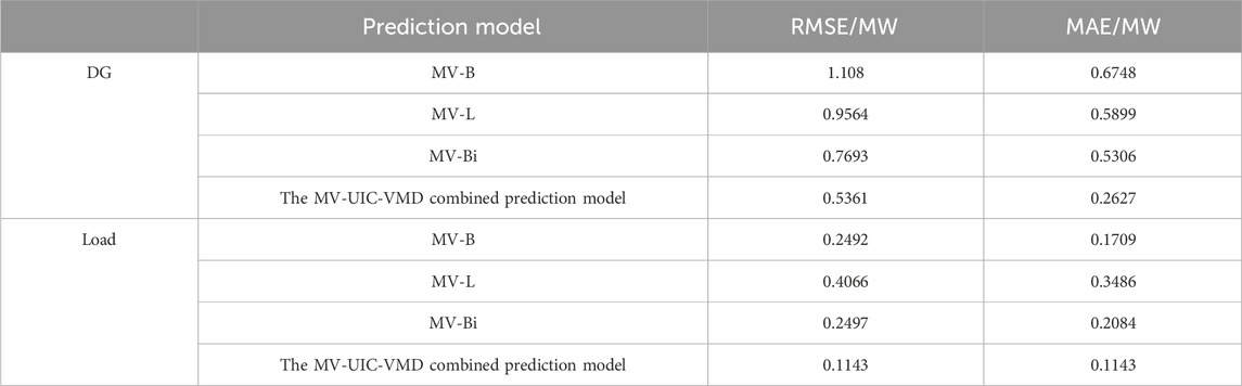
Table 6. Evaluation indexes of source and load power prediction models after dimensionality reduction of IEEE 118-bus standard distribution system.
5.4 Simulation case 4: with the prediction results that consider only the distributed power supply and load alone in correlation with the weather feature
For comparative analysis, the influence of weather features only on DG output and load power is set separately using the proposed algorithm to predict the load in the above two scenarios. The prediction results are shown in Figures 12, 13 and Table 7.
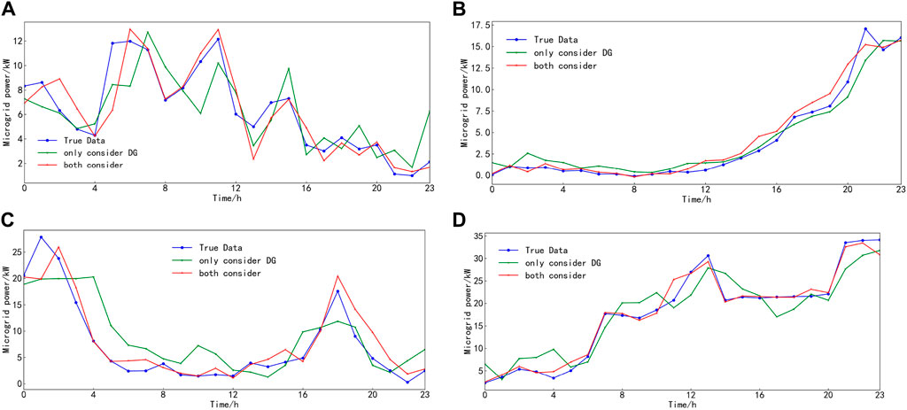
Figure 12. Only the predicted results of the DG output were considered. (A) Spring. (B) Summer. (C) Fall. (D) Winter.
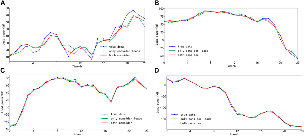
Figure 13. Only the predicted results of the loads were considered. (A) Spring. (B) Summer. (C) Fall. (D) Winter.
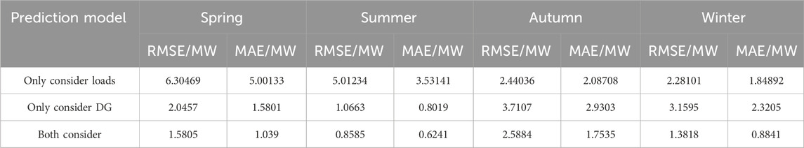
Table 7. Evaluation indexes of source and load power prediction models after dimensionality reduction.
Based on the simulations of the two scenarios mentioned above, it can be inferred that considering the correlation between DG output, load power, and weather characteristics can further improve the accuracy of load forecasting. Additionally, the proposed algorithm in this paper has a prediction time of 33.18 s, demonstrating good timeliness and meeting the requirements of ultra-short-term load forecasting.
6 Conclusion
In response to the coexistence of distributed power sources and loads in microgrids, wherein weather characteristics concurrently influence their power, a joint short-term power prediction model for microgrid sources and loads, considering weather features and multivariable correlations, is proposed to attain a rational match between microgrid sources and loads. Illustrated by an analysis of the DTU 7K 47-bus system within Denmark, an assessment of the accuracy, applicability, and efficacy of the proposed prediction approach is conducted. The principal findings are as follows:
(1) MV-UIC can effectively depict the simultaneous impact of the same weather characteristics on the power of sources and loads within microgrids, thereby revealing the correlation between weather features and microgrid power.
(2) By employing MV-UIC in conjunction with factor analysis to reduce the dimensionality of input features for source and load prediction, the power forecasting accuracy surpasses that achieved when considering all weather features as input. Compared to single prediction models, utilizing the prediction model based on MV-UIC-FA for source and load power also effectively reduces prediction errors.
Upon deriving the predicted power for microgrid sources and loads through the methodology advanced in this paper, the subsequent phase will involve the modeling of the matching degree between microgrid sources and loads, coupled with the optimization scheduling research of microgrid clusters.
Data availability statement
Publicly available datasets were analyzed in this study. This data can be found here: https://orbit.dtu.dk/en/datasets/dtu-7k-bus-active-distribution-network.
Author contributions
ZH: Conceptualization, Methodology, Visualization, Writing–original draft. NS: Supervision, Validation, Writing–review and editing. HS: Project administration, Writing–review and editing. YL: Funding acquisition, Resources, Writing–review and editing.
Funding
The author(s) declare that no financial support was received for the research, authorship, and/or publication of this article.
Conflict of interest
Author ZH was employed by State Grid Shandong Electric Power Company. Authors NS, HS, and YL were employed by State Grid Yantai Power Company.
Publisher’s note
All claims expressed in this article are solely those of the authors and do not necessarily represent those of their affiliated organizations, or those of the publisher, the editors and the reviewers. Any product that may be evaluated in this article, or claim that may be made by its manufacturer, is not guaranteed or endorsed by the publisher.
Supplementary material
The Supplementary Material for this article can be found online at: https://www.frontiersin.org/articles/10.3389/fenrg.2024.1409957/full#supplementary-material
References
Baviskar, A., Hansen, A. D., Das, K., and Douglass, P. J. (2021). “Open-source active distribution grid model with a large share of res-features, and studies,” in 2021 9th IEEE International Conference on Power Systems (ICPS), Kharagpur, India, 16-18 December 2021 (IEEE), 1–6. doi:10.1109/ICPS52420.2021.9670223
Chang, G. W., and Lu, H. J. (2018). Integrating gray data preprocessor and deep belief network for day-ahead PV power output forecast. IEEE Trans. Sustain. Energy 11 (1), 185–194. doi:10.1109/tste.2018.2888548
Hong, T., Pinson, P., Fan, S., Zareipour, H., Troccoli, A., and Hyndman, R. J. (2016). Probabilistic energy forecasting: Global energy forecasting competition 2014 and beyond. Int. J. Forecast. 32 (3), 896–913. doi:10.1016/j.ijforecast.2016.02.001
Hossain, M. S., and Mahmood, H. (2020). Short-term photovoltaic power forecasting using an LSTM neural network and synthetic weather forecast. Ieee Access 8, 172524–172533. doi:10.1109/access.2020.3024901
Jiang, F., Lin, Z., Wang, W., Wang, X., Xi, Z., and Guo, Q. (2023). Optimal bagging ensemble ultra short term multi-energy load forecasting considering least average envelope entropy load decomposition. Proc. CSEE 43 (08), 3027–3048. doi:10.13334/j.0258-8013.pcsee.223470
Kobayashi, K., and Iwai, M. (2018). Quantitative independent component selection using attractor analysis for noise reduction in magnetocardiogram signals. IEEE Trans. Magnetics 54 (11), 1–4. doi:10.1109/tmag.2018.2845903
Lin, Z. (2022). Short-term prediction of building sub-item energy consumption based on the CEEMDAN-BiLSTM method. Front. Energy Res. 10, 908544. doi:10.3389/fenrg.2022.908544
Masoumi, A., Jabari, F., Ghassem Zadeh, S., and Mohammadi-Ivatloo, B. (2020). Long-term load forecasting approach using dynamic feed-forward back-propagation artificial neural network. Optim. Power Syst. Problems Methods, Algorithms MATLAB Codes, 233–257. doi:10.1007/978-3-030-34050-6_11
Ma, W., Qiao, Y., Lu, Z., Li, J., Sun, S., and Zhou, Q. (2023). Short-term wind power prediction based on combination of screening and optimizing sensitive meteorological characteristics. Power Syst. Technol. 47 (07), 2897–2908. doi:10.13335/j.1000-3673.pst.2022.1515
Mousavi, A., and Baranuk, R. G. (2022). Uniform partitioning of data grid for association detection. IEEE Trans. Pattern Analysis Mach. Intell. 44 (2), 1098–1107. doi:10.1109/tpami.2020.3029487
Ng, D. T. K., Wu, W., Leung, J. K. L., and Chu, S. K. W. (2023). “Artificial Intelligence (AI) literacy questionnaire with confirmatory factor analysis,” in 2023 IEEE International Conference on Advanced Learning Technologies (ICALT), Orem, UT, USA, July 10-13, 2023 (IEEE), 233–235. doi:10.1109/ICALT58122.2023.00074
Qun, Y. U., Huo, X., He, J., Li, L., Zhang, J., and Feng, Y. (2023). Trend prediction of power blackout accidents in Chinese power grid based on spearman’s correlation coefficient and system inertia. Proc. CSEE 43 (14), 5372–5381. doi:10.13334/j.0258-8013.pcsee.220035
Ramirez, D., Santamaria, I., Scharf, L. L., and Van Vaerenbergh, S. (2019). Multi-channel factor analysis with common and unique factors. IEEE Trans. Signal Process. 68, 113–126. doi:10.1109/tsp.2019.2955829
Reshef, D. N., Reshef, Y. A., Finucane, H. K., Grossman, S. R., McVean, G., Turnbaugh, P. J., et al. (2011). Detecting novel associations in large data Sets. SCIENCE 334 (6062), 1518–1524. doi:10.1126/science.1205438
Safari, N., Chung, C. Y., and Price, G. (2018). Novel multi-step short-term wind power prediction framework based on chaotic time series analysis and singular spectrum analysis. IEEE Trans. power Syst. 33 (1), 590–601. doi:10.1109/tpwrs.2017.2694705
Wang, K., Wang, C., Yao, W., Zhang, Z., Liu, C., Dong, X., et al. (2024). Embedding P2P transaction into demand response exchange: a cooperative demand response management framework for IES. Appl. Energy 367, 123319. doi:10.1016/j.apenergy.2024.123319
Wang, T., Liang, H., Cao, J., and Zhao, Y. (2023). Probabilistic power flow calculation using principal component analysis-based compressive sensing. Front. Energy Res. 10, 1056077. doi:10.3389/fenrg.2022.1056077
Wang, Y. (2020). Algorithm analysis and improvement of maximum information coefficient. Xi'an: University of Electronic Science and Technology.
Wu, C., Sun, S., Cui, Y., and Xing, S. (2024). Driving factors analysis and scenario prediction of CO2 emissions in power industries of key provinces along the Yellow River based on LMDI and BP neural network. Front. Ecol. Evol. 12, 1362541. doi:10.3389/fevo.2024.1362541
Xu, W., Shen, Z., Fan, X., and Liu, Y. (2023). Short-term wind power prediction based on anomalous data cleaning and optimized lstm network. Front. Energy Res. 11, 1268494. doi:10.3389/fenrg.2023.1268494
Youssef, H. H., Mokhlis, H. B. I. N., Talip, M. S. A., Samman, M. A., Muhammad, M. A., and Mansor, N. N. (2020). Distribution network reconfiguration based on artificial network reconfiguration for variable load profile. Turkish J. Electr. Eng. Comput. Sci. 28 (5), 3013–3035. doi:10.3906/elk-1912-89
Yu, Y., Jin, Z., Ćetenović, D., Ding, L., Levi, V., and Terzija, V. (2024). A robust distribution network state estimation method based on enhanced clustering Algorithm: accounting for multiple DG output modes and data loss. Int. J. Electr. Power & Energy Syst. 157, 109797. doi:10.1016/j.ijepes.2024.109797
Yue, Y. U., Guo, J., and Jin, Z. (2023). Optimal extreme random forest ensemble for active distribution network forecasting-aided state estimation based on maximum average energy concentration VMD state decomposition. Energies 16 (15), 5659–5664. doi:10.3390/en16155659
Zhang, Z., Wang, C., Wu, Q., and Dong, X. (2024). Optimal dispatch for cross-regional integrated energy system with renewable energy uncertainties: a unified spatial-temporal cooperative framework. Energy 292, 130433. doi:10.1016/j.energy.2024.130433
Zhou, Y., Qian, C., Wang, Y., Wang, W., Zhou, J., and Wang, H. (2020). Feature parameter extraction of load model identification based on clustering algorithm and class noisy data. Adv. Technol. Electr. Eng. Energy 39 (12), 12–18. doi:10.12067/ATEEE200801
Zhu, Q., Jiateng, Li, Qiao, Ji, Shi, M., and Wang, C. (2023). Application and outlook of artificial intelligence technology in new energy power forecasting. Proc. CSEE 43 (08), 3027–3048. doi:10.13334/j.0258-8013.pcsee.213114
Keywords: weather characteristics, multivariable unified information coefficient, source and load power, joint prediction, machine learning
Citation: Huang Z, Sun N, Shao H and Li Y (2024) Ultra-short-term prediction of microgrid source load power considering weather characteristics and multivariate correlation. Front. Energy Res. 12:1409957. doi: 10.3389/fenrg.2024.1409957
Received: 31 March 2024; Accepted: 22 May 2024;
Published: 10 June 2024.
Edited by:
Yang Yu, Nanjing University of Posts and Telecommunications, ChinaReviewed by:
Kenneth E. Okedu, Melbourne Institute of Technology, AustraliaBowen Zhou, Northeastern University, China
Copyright © 2024 Huang, Sun, Shao and Li. This is an open-access article distributed under the terms of the Creative Commons Attribution License (CC BY). The use, distribution or reproduction in other forums is permitted, provided the original author(s) and the copyright owner(s) are credited and that the original publication in this journal is cited, in accordance with accepted academic practice. No use, distribution or reproduction is permitted which does not comply with these terms.
*Correspondence: Zhenning Huang, YWFhMTc0ODU1NjUxM0AxNjMuY29t