Evaluation of electrical load demand forecasting using various machine learning algorithms

The energy sector heavily relies on a diverse array of machine learning algorithms for power load prediction, which plays a pivotal role in shaping policies for power generation and distribution. The precision of power load prediction depends on numerous factors that reflect nonlinear traits within the data. Notably, machine learning algorithms and artificial neural networks have emerged as indispensable components in contemporary power load forecasting. This study focuses specifically on machine learning algorithms, encompassing support vector machines (SVMs), long short-term memory (LSTM), ensemble classifiers, recurrent neural networks, and deep learning methods. The research meticulously examines short-term power load prediction by leveraging Chandigarh UT electricity utility data spanning the last 5 years. The assessment of prediction accuracy utilizes metrics such as normalized mean square error (NMSE), root mean squared error (RMSE), mean absolute error (MAE), and mutual information (MI). The prediction results demonstrate superior performance in LSTM compared to other algorithms, with the prediction error being the lowest in LSTM and 13.51% higher in SVMs. These findings provide valuable insights into the strengths and limitations of different machine learning algorithms. Validation experiments for the proposed method are conducted using MATLAB R2018 software.

1 Introduction

Load forecasting serves as a crucial intermediary, ensuring a seamless connection between electricity generation and distribution. Its primary objective is to precisely forecast the electricity load for the upcoming year, months, and weeks, encompassing both short- and long-term projections. Effective power load forecasting enables the efficient management of power distribution scarcity. Demand forecasting also plays a pivotal role in driving nations’ industrialization and urban development (Lai et al., 2020; Aslam et al., 2021; Fan et al., 2019; Mosavi et al., 2019). Accurate forecasting is crucial for effective planning and promoting economic growth within a nation. The power load forecasting process relies on archived data and statistical models to predict future trends. However, the nonlinear nature of power generation data frequently leads to increased prediction errors, which can compromise decision-making regarding power generation and distribution. Despite the existence of numerous mathematical models for power load forecasting, attaining high accuracy in these forecasts remains a significant challenge (Su et al., 2019; Khan W. et al., 2020). Predicting the power load is a contemporary research focus. The advancement of machine learning (ML) algorithms propels the evolution of machine learning and its application in energy forecasting. The amalgamation of sensor technology with power distribution results in the accumulation of a significant volume of data. These amassed data present both opportunities and challenges for making informed decisions. In-depth data processing is conducted for evaluation and forecasting, with machine learning algorithms and models playing a pivotal role in prediction. Due to their efficiency and effectiveness, these algorithms and models have garnered considerable importance in predictive modeling for production, consumption, and demand analysis in recent years (Ahmad W. et al., 2020, Almaghrebi et al., 2020). Despite the extensive research conducted on machine learning and the advancements made in memory-based algorithms, innovative approaches have been proposed for predicting electricity demand. Several statistical functions have been used to model and forecast demand, including gray models, linear regression, autoregressive average models, and partial linear models, all of which are widely utilized in this field (Khan P. et al., 2020; Reynolds et al., 2019; O’dwyer et al., 2019). However, while strong predictive outcomes can generally be achieved, statistical methods are constrained by the underlying linear assumption. The gray prediction model operates without relying on statistical assumptions; nevertheless, its predictive accuracy depends on the dispersion level within the input time series (Chapaloglou et al., 2019; Bedi and Toshniwal, 2019; Jiang et al., 2020). Additionally, due to the distinctive strengths and limitations of each model, it is rare for a single forecasting model to maintain superiority in every situation. Another area of this study focuses on the evolution of load forecasting, transitioning from statistical to hybrid forecasting methods that integrate intelligent approaches capable of addressing complex and nonlinear challenges (Satre-Meloy et al., 2020; Wang R. et al., 2020; Ibrahim et al., 2020; Heydari et al., 2020). The implementation of the incremental approach design incorporates machine learning and artificial neural network algorithms (Ullah et al., 2020; Chammas et al., 2019; Santamouris, 2020; Sun et al., 2020). In contemporary data analysis research, both feed-forward neural networks and recurrent neural networks are extensively used across diverse models to achieve precise power load forecasting. The reliability of these predictions depends on the data processing methods used within the decision system. Among the different algorithms used in predictive models for electricity data, one involves the formation of data subsets in time series. Prevalent preprocessing techniques like singular spectrum analysis, ensemble empirical mode decomposition (EMD), and enhanced whole-ensemble empirical mode decomposition with adaptive noise are applied in analyzing electrical data modeling. These methods aid in establishing a procedural framework for extracting essential information from observed load series to forecast future patterns.

The utilization of EMD-based modeling has demonstrated success in managing electricity demand sequences. The research findings suggest that the EMD framework shows promise for accurately forecasting energy demand within specific intervals. Additionally, they developed feature selection techniques to improve the model’s performance. They also created a hybrid feature selection technique to extract fundamental knowledge from electricity time series. This finding underscores the importance of utilizing preprocessing techniques to improve predictions.

In addition to data, weather conditions significantly influence the precision of power load forecasting. Integrating various approaches and incorporating energy source guidelines lead to a new algorithm for short-term load prediction, significantly enhancing accuracy (Hu et al., 2020; Prado et al., 2020; El-Hendawi and Wang, 2020). This study investigated an approach to extracting date-associated details from observed load sequences and developed techniques for selecting features to enhance model effectiveness. Moreover, it introduced a hybrid technique to extract essential knowledge from electricity time-series data. It underscores the significance of preprocessing methods in refining predictions. Weather conditions can also impact power load forecasting, introducing complexities due to seasonal effects and reducing the accuracy of specific models. Consequently, many researchers suggest integrating seasonal pattern-effect models into predictive modeling to address this issue (Li et al., 2020; Qiao et al., 2020; Bakay et al., 2021).

The primary objective of this paper is to explore power load forecasting using artificial intelligence methods such as machine learning and artificial neural networks. The research aims to conduct experimental analyses on datasets using various machine learning algorithms to establish a model design for power load forecasting.

The remainder of the paper is structured as follows: Section II concentrates on recent advancements in power load forecasting; Section III outlines the machine learning approaches used for forecasting; Section IV offers an in-depth examination of the experimental methodology; and finally, Section V concludes the paper and offers insights into future directions for further exploration.

2 Related work

In the field of renewable energy forecasting, Lai et al. (2020) conducted a survey and evaluation of machine learning algorithms. Moreover, this work clarified the methodologies utilized in machine learning models for predicting sustainable energy sources, encompassing data preprocessing methods, attribute selection strategies, and performance assessment metrics. Additionally, the study scrutinized renewable energy sources, mean absolute error (MAE) percentages, and coefficients of determination. Aslam et al. (2021) provided a thorough examination of existing deep learning (DL)-based solar modules and wind turbine power forecasting approaches, along with a significant amount of data on electric power forecasting. The study included datasets used in training and validating various predictive models based on deep learning, facilitating the selection of appropriate datasets for new research projects. Fan et al. (2019) developed a novel short-term load prediction algorithm with improved accuracy using the weighted k-nearest neighbor technique. The forecast inaccuracies of this model are juxtaposed against those of the back-propagation neural network model and the autoregressive moving average (ARMA) model. Evaluation through correlation values demonstrates the capability of the proposed forecasting model to offer adaptable advantages, making it suitable for short-term demand forecasting. Mosavi et al. (2019) presented the current state of energy machine learning models, along with a new edition and application taxonomy. A novel methodology is used to identify and categorize machine learning models based on the method of machine learning simulations, the type of energy, and the application sector. Through the utilization of hybrid machine learning models, the efficiency, resilience, reliability, and generalization performance of machine learning models in energy systems have all significantly improved. Almaghrebi et al. (2020) utilized a dataset obtained from public charging stations over a span of 7 years in Nebraska, United States. The XGBoost regression model outperforms other techniques in forecasting charging requirements, showcasing an RMSE of 6.7 kWh and an R² of 52%. Reynolds et al. (2019) presented two approaches to improve district energy management. A heater set-point temperature is implemented to regulate building demand directly. Additionally, it assists in enhancing district heat production through a multi-vector energy hub. These observations underscore the potential benefits of comprehensive energy management, encompassing diverse energy vectors while considering both supply and demand aspects. Khan W. et al. (2020) presented machine learning techniques used to construct a hybrid power forecasting model. Extreme boosting, subcategory boosting, and the random forest (RF) technique are the four machine learning algorithms used. Our hybrid model enhances forecasting by employing feature extraction to preprocess data. While machine learning algorithms are frequently effective in handling high-energy situations, our hybrid version improves forecasts by utilizing feature engineering to preprocess data. Ahmad W. et al. (2020) proposed a groundbreaking deep learning-based technique for forecasting electrical loads. Additionally, a three-step model is developed, incorporating a hybrid feature selector for feature selection, a feature extraction technique to reduce redundancy, and improved support vector machines (SVMs) and extreme learning machines (ELMs) for classification and forecasting. Numerical simulations are graphed, and statistics are presented, suggesting that our upgraded methods are more accurate and perform better than state-of-the-art approaches. Bedi and Toshniwal (2019) proposed acquiring season-based segmentation data and developed a deep learning method for projecting electricity usage while accounting for long-term historical dependency. First, the monthly electricity use data are utilized to conduct cluster analysis. Subsequently, load trends are characterized to enhance the comprehension of the metadata encompassed within each cluster. Jiang et al. (2020) provided forecast intervals that represent the intricacies involved in the design and functioning of power systems with better accuracy. The findings suggest that the suggested model demonstrates encouraging forecasts compared to alternative combined methodologies, which can be advantageous for policymakers and public organizations aiming to maintain the security and stability of the energy infrastructure. Wang R. et al. (2020) proposed a useful enhancement integration-model stacking structure designed to address increasing energy needs. To ensure the comprehensive observation of datasets from diverse spatial and structural perspectives, the stacking model harnesses the strengths of multiple base prediction algorithms, transforming their outcomes into “meta-features.” With accuracy gains of 9.5% for case A and 31.6%, 16.2%, and 49.4% for case B, the stacking method outperforms earlier models. Heydari et al. (2020) proposed an innovative and accurate integrated model designed for short-term load and price forecasting. This comprehensive package incorporates the gravitational search algorithm, variational mode decomposition, mixed data modeling, feature selection, and generalized regression neural networks. The proposed model surpasses current benchmark prediction models in terms of precision and stability, as indicated by the findings. Wang et al. (2019) analyzed the systems in depth for forecasting renewable energy based on deep learning methodologies to determine their efficacy, efficiency, and relevance. Additionally, to improve forecasting accuracy, various data preparation strategies and mistake post-correction processes are examined. Several deep learning-based forecasting algorithms are thoroughly investigated and discussed. Sun et al. (2020), in their comprehensive examination, delved deeply into forecasting energy use in buildings. Their meticulous analysis encompasses feature manipulation, potential data-centric models, and projected outcomes, thus encompassing the entirety of the data-driven procedure. In a research project, Ahmad and Chen (2019a) explored short-term energy demand predictions at the district level. They employed two distinct deep learning models. These DL models exhibited higher predictive accuracy at distinct hidden neurons, attributed to the suggested network layout. Hu et al. (2020), utilizing a novel augmented optimization model, constructed and refined it using a differential evolution methodology developed through the bagged echo state network approach. Bagging, a network generalization technique, enhances network generalization while reducing forecasting errors. The suggested model, known for its high precision and reliability, proves to be a valuable method for predicting energy consumption. Walker et al. (2020) explored various machine learning algorithms across a spectrum to estimate the electricity demand in hourly intervals, both at the individual building and aggregated levels. Upon factoring in processing time and error accuracy, the results revealed that random forest and artificial neural network (ANN) models yielded the most accurate predictions at an hourly granularity. Prado et al. (2020) employed methodologies such as the fuzzy inference system model, auto-regressive integrated moving average, support vector regression, adaptive neuro-fuzzy inference system, ANN, ELM, and genetic algorithm. In a sample study, compared to leading artificial intelligence and econometric models, the proposed method attained a 22.3% reduction in the mean squared error and a 33.1% decrease in the mean absolute percentage error. Ahmad et al. (2020a) reported that utility companies require a stable and reliable algorithm to accurately predict energy demand for multiple applications, including electricity dispatching, market involvement, and infrastructure planning. The forecasting results assist in enhancing and automating predictive modeling processes by bridging the gap between machine learning models and conventional forecasting models. El-Hendawi and Wang (2020) introduced the whole wavelet neural network methodology, an ensemble method that incorporates both the overall wavelet packet transform and neural networks. This approach utilizes both components effectively. The proposed methodology has the potential to assist utilities and system operators in accurately predicting electricity usage, a critical aspect for power generation, demand-side management, and voltage stability operations. Zhang et al. (2021) proposed utilizing machine learning approaches for load prediction within the framework of machine learning. The objective is to accomplish tasks through performance measures and learning from past experiences. They conclude with a list of both well-studied and under-explored sectors that warrant further investigation. The research introduces a neural network model specifically designed to predict short-term loads for a Colombian grid operator spanning a week. The model employs a long short-term memory (LSTM) recurrent neural network and historical load data from a specific region in Colombia. The performance of the model is evaluated using the regression metric MAPE, with the most accurate week displaying an error rate of 1.65% and the least accurate week exhibiting an error rate of 26.22% (Caicedo- Vivas and Alfonso-Morales, 2023). This research introduces a method for reconstructing input features utilizing the maximum information coefficient (MIC). The procedure commences by categorizing load curves through distributed photovoltaic systems (DPVSs) with Gaussian mixture model (GMM) clustering. The presented case study illustrates how this proposed feature reconstruction method significantly enhances the prediction accuracy of deep neural networks (Zheng et al., 2023). The study suggests utilizing long short-term memory Bayesian neural networks for forecasting household loads, especially in scenarios involving EV charging. The findings demonstrate a comparable level of accuracy to point forecasts, coupled with the advantage of providing prediction intervals (Skala et al., 2023).

Pawar and Tarunkumar (2020), within a smart grid featuring a significant renewable energy presence, recommended using an intelligent smart energy management system (ISEMS) to meet energy demands. To achieve accurate energy estimations, the proposed approach compares various prediction models, focusing on both hourly and daily planning. Among these models, the particle swarm optimization (PSO)-based SVM regression model demonstrates superior performance accuracy. Fathi et al. (2020) showed how change impacts the energy efficiency of urban structures using machine learning methods and future climate simulations. Due to the absence of a globally applicable metric for this assessment, determining the most reliable machine learning-based forecast requires an optimal combination of criteria. Somu et al. (2021) suggested that KCNN-exact LSTM holds promise as a deep learning model for forecasting energy demand owing to its capability to recognize spatial and temporal associations within the dataset. To evaluate its dependability, the KCNN-LSTM model was compared against the k-means variant of established electricity usage-pattern forecast models using recognized quality criteria. Ahmad and Chen (2019b), by using genuine pollution data and sustainable consumption records, applied NARM, LMSR, and LS Boost methodologies to forecast the energy demands of large-scale urban utilities, utility firms, and industrial customers. Throughout the summer, fall, winter, and spring periods, the LS Boost model showcased coefficients of variation of 5.019%, 3.159%, 3.292%, and 3.184%, respectively. Ahmad and Chen (2020) conducted a thorough assessment and compared several simulations to select the best forecasting model for obtaining the required result in a number of situations. With coefficients of correlation of 0.972 and 0.971, respectively, the Bayesian regularization backpropagation neural networks and Levenberg Marquardt backpropagation neural networks provide better forecasting accuracy and performance. Ahmad et al. (2020b) used renewable energy and electricity projection models as a key and systematic energy planning tool. The forecast periods are segmented into three separate classifications: short-range, intermediate-range, and long-range. The outcomes of this study will aid practitioners and researchers in recognizing prediction methodologies and selecting relevant methods for achieving their desired goals and forecasting criteria. Choi et al. (2020) developed, in response to the recent power demand patterns, a unique load demand forecasting system constructed using LSTM deep learning techniques. They performed examinations to gauge the inaccuracies of the forecasting module and unexpected deviations in the energy usage patterns within the real-time power demand monitoring system. Su et al. (2019) investigated the ANN, SVM, gradient boosting machines (GBM), and Gaussian process regression (GPR) as examples of data-driven predictive models for natural gas price forecasting. To train the model, quarterly Henry Hub natural gas market pricing data and a pass approach are utilized. These two machine learning algorithms operate differently in predicting natural gas prices, with the ANN demonstrating superior prediction accuracy over the SVM, GBM, and GPR, according to the data. Khan P. et al. (2020) proposed utilizing a variety of data mining approaches, such as preprocessing past demand data and analyzing the properties of the load time series, to examine patterns in energy usage from both renewable and non-renewable energy sources. O’dwyer et al. (2019) investigated recent advancements in the smart energy sector, focusing on methodologies in key application areas and notable implemented examples. They also highlight significant challenges in this sector while outlining future prospects. The aim of this inquiry is to assess the current state of computational intelligence in smart energy management and provide insights into potential strategies to overcome current limitations. Chapaloglou et al. (2019) proposed that smoother diesel generator performance can be achieved by combining it with peak shaving using renewable energy. This approach aims to reduce the demand variability that conventional units must meet. The operation seeks to limit the maximum capacity of diesel engines while simultaneously increasing the supply of renewable energy to the grid. Satre-Meloy et al. (2020) applied a unique dataset containing significant strength and tenant time-use data from United Kingdom homes. They also utilized a groundbreaking clustering approach to capture the entire structure. The discussion focuses on how a customized strategy tailored to the highest demand in residential areas can lead to reductions in demand and mitigation actions. Additionally, it enhances our understanding of the limitations and possibilities for demand flexibility in the household sector. Ibrahim et al. (2020) reported that the increasing interest in machine learning technologies underscores their effectiveness in tackling technological challenges within the smart grid. However, certain hurdles, such as efficient data collection and the examination of intelligent decision-making in complex multi-energy systems, as well as the need for streamlined machine learning-based methods, remain unresolved. Ullah et al. (2020) provided comprehensive insights into the utilization of previous advancements in intelligent transportation systems (ITSs), cybersecurity challenges, the effective use of smart grids for energy efficiency, optimized deployment of unmanned aerial vehicles to enhance 5G and future communication services, and the integration of smart medical systems within the framework of a smart city. Chammas et al. (2019) proposed that LR, SVM, GBM, and RF are four alternative classification algorithms compared to our methodology. A multilayer perceptron (MLP)-based system for calculating the energy consumption of a building based on data from a wireless sensor network (WSN), including luminosity, day of the week, moisture, and temperature, significantly influences the outcomes observed in the testing set. This yields cutting-edge outcomes with a coefficient of determination R² of 64% , RMSE of 59.9%, MAE of 27.3%, and MAPE of 28.04%. Santamouris (2020) reported on energy, peak electricity usage, air pollution, mortality, morbidity, and urban susceptibility. The study also examined recent data on the characteristics and extent of urban overheating, as well as analyses of recent research on the connection between urban heat islands and increasing temperatures. Li et al. (2020) estimated that an SVM and an upgraded dragonfly algorithm are utilized to generate short-term wind electricity forecasts. To enhance the performance of the standard dragonfly approach, an adaptive learning multiplier and a convex optimization strategy are proposed. The suggested model outperforms existing methods, such as MLP networks and Gaussian process models, in terms of forecast precision. Lu et al. (2019) proposed that residential management systems utilize an hour-ahead load management algorithm. A stable pricing methodology derived from artificial neural networks is suggested to address the complexities of future pricing. Calculations involving non-shiftable, shiftable, and guided loads are used to validate the performance of the suggested energy management method (Fathi et al., 2020). Wang H. et al. (2020) carried out a classification study using AI algorithms and current solar power prediction models. Taxonomy is a system for classifying solar energy forecasting methods, optimizers, and frameworks based on similarities and differences. This study can aid scientists and engineers in conceptually analyzing various solar forecast models, allowing them to select the most appropriate model for any given usage scenario. Ghoddusi et al. (2019) proposed that in energy economics publications, SVMs, ANNs, and genetic algorithms (GAs) are among the most commonly utilized methodologies. They explored the successes and limitations of the literature. Gao et al. (2019) provided a prediction method based on the weather conditions of previous days for optimal weather conditions. According to a study of predictive accuracy between new methods and known algorithms, the RMSE accuracy of the predicting approach that is built upon LSTM networks can achieve 4.62%, specifically under ideal weather conditions. Xue et al. (2019) proposed the ability to forecast the best weather conditions; here, a method based on the previous-day climatic data is used. The RMSE accuracy of LSTM infrastructure-predicting approaches can reach 4.62% for favorable climatic circumstances, according to research on the projected accuracy between innovative approaches and known algorithms. Qiao et al. (2020) presented a hybrid approach for carbon dioxide emission forecast that combines the lion swarm optimizer with the genetic algorithm to improve the traditional least squares support vector machine model. When compared with eight previous methods, the novel algorithm demonstrates superior global optimization capabilities, quicker convergence, enhanced accuracy, and moderate computational speed. Bakay et al. (2021) reported that measurements of CO₂, CH₄, N₂O, F-gases, and overall GHG emissions from the energy-generating industry can be predicted using DL, SVM, and ANN approaches. All of the algorithms tested in the study, according to the findings, yielded individually favorable outcomes in predicting GHG emissions. The greatest R² value for emissions, according to the expected data, ranges from 0.861 to 0.998, and all conclusions are considered “excellent” regarding the RMSE. Zhou et al. (2019), in their analysis, comprehensively assessed prior driving prediction techniques, highlighting suitable application scenarios for each prediction model. Moreover, it outlines methods to address prediction inaccuracies, aiding designers in selecting suitable driving prediction techniques for varied uses and improving the efficiency of predictive energy management strategies for hybrid and plug-in hybrid electric vehicles. Hao et al. (2019) introduced the DE clustering technique, derived from fundamental morphological processes, to recognize days sharing analogous numerical weather prediction data with the envisaged day within the suggested approach. The progressive generalized regression neural network (GRNN) prediction framework rooted in the DE clustering technique demonstrates superior efficacy in forecasting wind power for the following day compared to the models utilizing DPK clustering-GRNN, AM-GRNN, and K-means clustering-GRNN. Ahmed et al. (2020) discovered that artificial neural network ensembles are the best for generating short-term solar power forecasts, that asynchronous sequential extreme learning machines are the best for adaptive networks, and that the bootstrap procedure is the best for assessing uncertainty When paired with hybrid artificial neural networks and evolutionary algorithms, the findings bring up new possibilities for photovoltaic power forecasting. Antonopoulos et al. (2020) provided a look at how AI is employed in disaster recovery applications. The study categorizes research based on the AI/ML algorithms employed and their applications in energy DR. It culminates by summarizing the strengths and weaknesses of the AI algorithms applied in diverse DR tasks, along with proposing avenues for future research in this burgeoning field (Fathi et al., 2020). Shaw et al. (2019) presented the predictive anti-correlated placement algorithm as a revolutionary algorithm that improves CPU and bandwidth usage. It relies on a comparative analysis of the most commonly utilized prediction models, placed alongside each other for comparison. The practical outcomes illustrate that the suggested approach conserves 18% of energy while reducing service violations by more than 34%, in contrast to several frequently used placement algorithms. Hou et al. (2021) analyzed the impact on energy production, demand, and greenhouse gas emissions. Climate scenario representative concentration pathways (RCPs) are used to project changes in weather elements because of this. Taking into account scenarios RCP2.6, RCP4.5, and RCP8.5, hydro-power production is anticipated to increase by approximately 2.765 MW, 1.892 MW, and 1.219 MW, respectively, in the foreseeable future. Furthermore, the projections suggest a subsequent increase to approximately 3.430 MW, 2.475 MW, and 1.827 MW, respectively. Jørgensen et al. (2020) discovered distinct characteristics in neural networks and support vector machines, which, if modified incorrectly, will cause mistakes. The algorithms can be adjusted to match a variety of situations owing to the many parameters. A growing trend involves utilizing machine learning to digitize wind power estimations.

2.1 Research gap

This project addresses the shortcomings observed in current research, outlined as follows:

Despite the considerable potential offered by ML and DL algorithms, the inherent variability among different techniques remains unexplored. Many investigations focus solely on LSTM, SVM, and EM without comparing their effectiveness against traditional deep learning approaches.

Furthermore, several studies fail to consider methods that showcase the resilience of assessed models, with cross-validation being underutilized. Consequently, the results presented often exhibit significant dependency on the specific data sample used, thereby limiting reproducibility and applicability to future datasets.

3 Methodology

3.1 Data preprocessing

Various machine learning methodologies heavily depend on the caliber and arrangement of the dataset. Implementing efficient preprocessing techniques, which encompass variable selection, data filtration, and transformation into an understandable format for the models, holds paramount significance. Throughout the data collection phase, inaccuracies in communication or gathering frequently result in absent values in the final dataset. Moreover, monitoring programs often capture a myriad of parameters, not all of which contribute to accurately predicting the target variable. To discern the most suitable dataset, a feature extraction procedure is utilized. This involves visually delineating the curves of various variables influencing the target feature through plotting. Additionally, this phase enables the extraction of information not explicitly present as variables but impacting the variability of the target feature, such as the hour of the day, day of the week, or day of the year. Typically, the chosen dataset encompasses weather conditions and electrical load data, with temporal parameters including the hour of the day, day of the week, and day of the year. Consequently, the objective is to forecast the output variable, electrical loads, based on the input variables selected due to their inherent correlation with variations across different time intervals. Specifically, the hour of the day facilitates the extraction of daily patterns, the day of the week reveals weekly patterns, and the day of the year aids in recognizing seasonal patterns.

Improving pattern recognition from the models is accomplished through a data-cleansing phase. Here, the data undergo filtration to identify outliers. Given the substantial instantaneous variability in electricity consumption, the methodology predominantly relies on the interquartile range. This iterative process aims to alleviate errors introduced by anomalous values in the trends. Consequently, values deviating outside the ranges defined by specific criteria are deemed invalid.

$\text{ub}=\mathrm{Q}3+1.5*\text{\hspace{0.17em}IQR},$

$\text{lb}=\mathrm{Q}1-1.5*\text{\hspace{0.17em}IQR},$

where “ub” and “lb” represent the upper bound and lower bound, respectively; “Q3” and “Q1” denote the third and the first quartiles, respectively; and “IQR” signifies the interquartile range. Values recognized as outliers, in addition to non-existent values within the dataset, are regarded as absent. Data preprocessing serves as the initial stage in machine learning, involving the transformation or encoding of data to prepare them for efficient analysis by the machine. Essentially, this process ensures that the data are in a format that enables the model algorithm to effectively interpret their features.

Data preprocessing holds significant importance for the generalization performance of supervised machine learning algorithms. As the dimensionality of the input space increases, the volume of training data increases exponentially. It is estimated that preprocessing tasks can consume up to 50%–80% of the overall classification process time, underscoring their critical role in model development. Enhancing data quality is also essential for optimizing performance.

The detailed steps of data preprocessing are outlined below.

3.1.1 Data cleaning and validation

Data cleansing involves the identification and rectification or removal of incorrect or noisy data from the dataset. It typically focuses on detecting and replacing incomplete, inaccurate, irrelevant, or other erroneous data and records. Duplicates can frequently occur in datasets, particularly when combining data from various sources, scraping data, or aggregating data from multiple clients. This situation presents an opportunity for the generation of duplicate data.

It is common for certain columns in a dataset to have missing values, which can arise from data validation rules or data collection processes. However, addressing missing values is essential, as they can impact the efficacy of the features of a model. When a significant number of values are missing, straightforward interpolation methods can be used to address these gaps. One of the most prevalent approaches involves using mean, median, or mode values based on the features of the model.

Missing data may result from human error or be generated while working with primary data. Therefore, it becomes necessary to have a data assessment process to learn the datatype of the feature and ensure that all data objects are of the same type. Inconsistent data might lead to erroneous conclusions and forecasts.

3.1.2 Regression (noise handling)

If noise persists within a class even after identifying loud occurrences, there are three strategies for addressing it. First, noise can be disregarded if the model exhibits robustness against overfitting. Second, noise in the dataset can be filtered out, adjusted, refined, or re-labeled. If the attribute-related noise persists, methods such as filtering or refining the erroneous attribute value, excluding it from the dataset, or utilizing imputation techniques can help identify areas requiring cleaning and unveil additional questionable values. This supervised machine learning technique is used for predicting continuous variables by establishing relationships between variables and estimating how each variable influences the others. To assess the predictions made by regression algorithms, it is essential to consider variance and bias metrics.

3.1.3 Data integration

Data integration refers to the amalgamation of data sourced from multiple origins into a unified dataset. This encompasses schema integration, which entails merging metadata from diverse sources and addressing discrepancies in data values stemming from variations in units of measurement, representation, and other factors. Additionally, it is essential to manage redundant data by employing techniques such as correlational analysis to uphold high data quality post-integration.

3.1.4 Data transformation (normalization)

Normalization becomes necessary when attributes are measured on different scales. In cases where multiple features exhibit distinct scales, normalization is essential to standardize them or risk yielding suboptimal outcomes. This process encompasses techniques such as min–max normalization, z-score normalization, and decimal scaling.

3.2 Machine learning algorithm modeling

Anticipating the load on power grids poses a significant obstacle within the energy industry in the current decade. Machine learning algorithms provide frameworks for analyzing the production, consumption, and distribution of power. With the coupling of supervised and unsupervised learning, machine learning derives thousands of algorithms as single and multiple predictive models for forecasting. The development of machine learning focuses on the accuracy and effectiveness of algorithms. The accuracy of the algorithms varies according to the sampling of energy data and modeling. The fundamental principle behind machine learning algorithms involves selecting past power load data as training samples, creating an appropriate network structure, and employing learning algorithms to predict the energy needs within the power sector. Figure 1 illustrates the process of applying machine learning models to power load data.

Figure 1

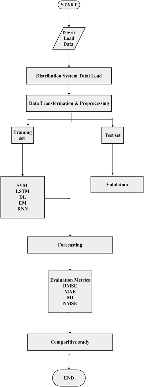
Figure 1. Flowchart for power load forecasting with machine learning algorithms.

The training phase involves a cross-validation approach to ensure the efficacy of the applied models. This method is used to ensure that each split produces results independent of the training, thereby minimizing overfitting in the modeling. Consequently, the training process occurs in one partition, comprising 80% of the training data, while the model’s performance is assessed in another partition, encompassing the remaining training data. This iterative process involves alternately positioning the validation subset throughout the training dataset.

Moreover, the training process utilizes mini-batch gradient descent to prevent stagnation at local minima and enhance the model’s convergence [47]. Upon completion of the training phase with these techniques, the model undergoes evaluation on the test dataset. This section examines the capabilities and assesses the suitability of various ML and DL models for electricity load forecasting.

The fundamentals of ML models are presented, commencing with SVM, followed by recurrent neural networks (RNNs) and LSTM. Subsequently, the distinctive features of the DL model and ensemble classifier are introduced.

The various algorithms applied in this study are described as follows.

3.2.1 Support vector machine

The SVM learning algorithm was formulated in 1990 and has since found extensive application in forecasting and pattern recognition tasks. Schematic Diagram of Support Vector Machine is shown in Figure 2. SVM learns to estimate input data on a regression line with a designated threshold. In this model, the ideal trend line that best fits the data is referred to as the hyperplane, while the boundary lines delineate the threshold. SVM maps training data using mathematical equations, called kernels, to determine the hyperplane containing the maximum input data within the boundary lines. It can exhibit linear, nonlinear, or sigmoid characteristics. In nonlinear SVM, the feature data undergo mapping from one plane to another, and data points are segregated in a nonlinear manner, with the decision factor determined by the margin function of the support vector.

Figure 2

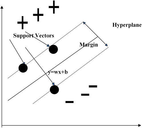
Figure 2. Schematic diagram of the support vector machine.

$\frac{1}{\left|\mathrm{w}\right|}$ is the margin. The concept of SVM revolves around maximizing the margin, as given in Eq. 1

$\mathrm{Max}\left(\frac{1}{‖\mathrm{w}‖}\right).(1)$

This concept can be expressed as shown below in Eq. 2

$\mathrm{Min}‖\mathrm{w}‖.(2)$

The hyperplane for the equation is acquired in the following manner, as given in Eq. 3 (Jiang et al., 2020; Satre-Meloy et al., 2020; Wang R. et al., 2020; Ibrahim et al., 2020):

$\mathrm{w}.{\mathrm{x}}_{\mathrm{i}}+\mathrm{b}\ge 1,\text{if\hspace{0.17em}}{\mathrm{y}}_{\mathrm{i}}=+1,$

$\mathrm{w}.{\mathrm{x}}_{\mathrm{i}}+\mathrm{b}\le -1,\text{if\hspace{0.17em}}{\mathrm{y}}_{\mathrm{i}}=-1.(3)$

Here, w is the weight vector, x is the input vector, and b is the bias.

The formula for minimizing the support vector is as follows and given in Eqs 4, 5:

$\min \frac{{‖\mathrm{w}‖}^2}{2}+\mathrm{C}.\frac{1}{\mathrm{n}}{\displaystyle \sum _{\mathrm{i}=1}^{\mathrm{n}}}{\mathrm{\xi }}_{\mathrm{i}},(4)$

${\mathrm{y}}_{\mathrm{i}}\left(\mathrm{w}.{\mathrm{x}}_{\mathrm{i}}+\mathrm{b}\right)\ge 1-{\mathrm{\xi }}_{\mathrm{i}},{\mathrm{\xi }}_{\mathrm{i}}\ge 0,(5)$

where ξ_i is some units of distance away from the correct hyperplane in the incorrect direction.

“C” is the hyperparameter, which is always a positive value. If C increases, the acceptance of out-of-bound values also escalates. Conversely, as C approaches 0, tolerance diminishes, thereby simplifying the issue and, hence, neglecting the impact of slack.

SVM emerges as a robust machine learning algorithm with promising benefits for electricity load forecasting, owing to several key factors.

- Nonlinearity: SVM adeptly captures complex, nonlinear relationships between electricity consumption and relevant features.

- Outlier resilience: Its design provides inherent robustness against outliers, ensuring stable performance even in the presence of anomalous data points.

- Flexibility: SVM offers adjustable parameters that enable fine-tuning to strike a balance between model complexity and generalization, thereby enhancing adaptability to fluctuations in electricity data.

- Handling high-dimensional data: SVM demonstrates efficacy in handling datasets with a large number of features without compromising its predictive performance.

3.2.2 Recurrent neural network

The RNN is a specialized form of the artificial neural network specifically crafted to analyze sequential time-series data. A key advantage of RNNs lies in their capability to process signals in both forward and backward directions. This is possible by creating network loops and allowing internal connections between hidden components. Due to their internal connections, RNNs are especially adept at utilizing information from preceding data to anticipate future data. Moreover, RNNs enable the exploration of temporal correlations among different datasets (Wang et al., 2019; Wang et al., 2020; H. Ghoddusi et al., 2019). Figure 3 shows the processing of the RNN.

Figure 3

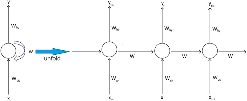
Figure 3. Process diagram of the recurrent neural network.

The input to an RNN cell at time step t is typically symbolized as x_t, and the hidden state at time step t is designated as h_t. The output at time step t is denoted as y_t. The cell is also equipped with parameters, such as weights and biases, denoted as W and b, respectively.

Every concealed layer operates based on two inputs: X_t and H_t−1. The output Y_t is influenced by the input from the hidden layer (h_t) at time t. These two functions are articulated in Eqs 6, 7 as follows:

$h_t=f_h\left(x_t,h_{t-1}\right),(6)$

$\widehat{y_t}=f_o\left(h_t\right).(7)$

The input, output, and concealed state of an RNN cell are typically computed using the subsequent Eqs 8, 9:

$h_t={\varphi }_h\left(W_{xh}.x_t+W_{hh}.h_{t-1}+b_h\right),(8)$

$\widehat{y_t}={\varphi }_o\left(W_{yh}.h_t+b_y\right).(9)$

In the transition hidden-layer function of ∅_h, a nonlinear activation function, like a sigmoid or tanh function, is typically incorporated.

The function ∅_o is a nonlinear activation function, such as a rectified linear unit (ReLU), and is derived by computing the dot product of the output weight with the hidden layer h_t and then adding the bias term.

RNNs present numerous advantages for electricity demand forecasting, including the following:

1. Adaptability: RNNs can accommodate variable-length input sequences, making them flexible in handling datasets with missing data.

2. Resilience: RNNs demonstrate robustness against noise and outliers present in the data. They possess the capability to detect and filter out irrelevant patterns, ensuring reliable forecasting outcomes.

3. Global context awareness: RNNs capture global information and dependencies across various time scales, allowing for a comprehensive understanding of the underlying patterns influencing electricity consumption.

4. Interpretability: RNN architectures facilitate better comprehension of the patterns contributing to electricity consumption, enhancing the interpretability of forecasting models.

3.2.3 Long short-term memory

The LSTM architecture was initially proposed by Schmidhuber in 1997 (Wang R. et al., 2020). Since its inception, the LSTM architecture has undergone subsequent developments by different researchers (Xue et al., 2019). LSTM was originally devised to combat the issue of vanishing gradients encountered in typical recurrent neural networks when handling long-term dependencies. Unlike a regular RNN, the hidden layers of LSTM possess a more intricate structure, consisting of a sequence of recurring modules. Each hidden layer within LSTM incorporates gate and memory cell concepts. The memory block includes four key elements: an entry gate, an exit gate, a self-connected memory cell, and a deletion gate. The entry gate regulates the activation of the memory cell, while the exit gate controls when to transfer information to the next network layers. Meanwhile, the deletion gate aids in discarding previous input data and resetting the memory cells. Additionally, multiplicative gates are strategically utilized to enable memory cells to retain information over extended periods. This specific architectural design significantly mitigates the vanishing gradient problem encountered in traditional RNNs (Hu et al., 2020; Qiao et al., 2020).

The LSTM features an input x(t), which can originate from either the output of a CNN or the input sequence directly. h _t−1 and c_t−1 are the inputs from the LSTM of the previous time step. o_t is the output of the LSTM for this time step. The LSTM also produces c_t and h_t for use by the LSTM in the next time step.

The forget gate f_t, as provided in Eq. 10, decides which previously stored information to maintain or discard upon receiving new data:

$f_t={\sigma }_g\left(W_f.x_t+U_f.h_{t-1}+b_f\right),(10)$

where σ_g is the activation function. The sigmoid activation function is commonly utilized because it condenses information within the interval [0, 1]. This allows the gate to determine the importance of information, for example, whether the value is close to or equals 1, indicating significance, or close to or equals 0, implying insignificance.

The input gate decides which fresh information to retain in the cell state. Initially, Eq. 11 determines what information needs updating i_t.

$i_t={\sigma }_g\left(W_i.x_t+U_i.h_{t-1}+b_i\right).(11)$

Via Eq. 12, the sequence, $c_t^{\prime }$, is regulated. Like the forget gate, the sigmoid activation function is often employed to retain essential information.

$c_t^{\prime }={\sigma }_c\left(W_c.x_t+U_c.h_{t-1}+b_c\right).(12)$

By amalgamating the outcomes of the aforementioned gates with the previously retained information in the cell state, c_t−1, the value of the cell state denoted by c_t, as provided in Eq. 13, undergoes modification.

$c_t=f_t{c}_{t-1}+i_t{c}_t^{\prime }.(13)$

Ultimately, the output gate dictates the output of the neuron. This result integrates the previously stored information with the fresh data and details obtained from the cell state, as shown in Eq. 14:

$o_t={\sigma }_g\left(W_o.x_t+U_o{h}_{t-1}+b_o\right),(14)$

$h_t=o_t{\sigma }_c\left(c_t\right).(15)$

The activation function governing the cell state σ_c is described in Eq. 15. The tanh activation function is used to allocate weights to these maintained values.

LSTM networks stand out for their ability to excel in scenarios reliant on temporal data, making them particularly advantageous for electricity load forecasting. The key advantages of LSTM include

1. Temporal modeling prowess: LSTM architectures are specifically tailored to model temporal dependencies in data, making them well-suited for time-series prediction tasks.

2. Context preservation: With their long short-term memory, LSTM networks can effectively capture short-term dependencies while accommodating irregular or missing data points. Additionally, they possess the capability to grasp long-term dependencies within the data.

3. Scalability: LSTM networks demonstrate effectiveness in capturing complex patterns from extensive historical data, enabling robust forecasting in scenarios with diverse and extensive datasets.

4. Robustness: LSTM architectures exhibit resilience against noise and outliers present in the data, ensuring reliable forecasting outcomes even in the presence of data irregularities.

3.2.4 Deep learning

The potential impact of deep learning on power load forecasting methods is substantial. Deep learning is a sub-field of machine learning, which is based on artificial neural networks. In the energy domain, the precision of power consumption prediction is significantly impacted by the processing of forecasted data, making deep neural networks highly relevant. In general, neural networks, better known as MLP, also referred to as feed-forward artificial neural networks, consist of multiple layers that establish connections between the input and output (Ahmed et al., 2020). Each layer comprises its own set of neurons. The number of input neurons typically aligns with the number of features, while the number of output neurons corresponds to the variables to be predicted. The quantity of hidden neurons and layers varies based on the specific problem. As the number of hidden layers or neurons increases, the model’s ability to extract complex patterns improves, albeit at the expense of heightened complexity. In such scenarios, the internal operations of the neurons rely on the activation of preceding neurons.

This progression extends from the input layer to the output layer through the neural interconnections. Moreover, if a node possesses multiple inputs, the final value of its function is the sum of the individual values of its functions and their connections. Each iteration of the training process concludes with backward propagation, where the error is disseminated back to the input layers and the weights are adjusted.

In many deep learning problems, we aim to predict an output z using a set of variables X. In this scenario, we assume that for each row of the database Xi, there exists a corresponding prediction z, as given in Eqs 16, 17:

$z=\sum w_i{x}_i+b_i,(16)$

$a=\psi \left(z\right),(17)$

where b_i is the bias. W_i is the weight. ψ is the activation function. “a” is the final output.

Deep learning emerges as a widely employed model, highly conducive to electricity consumption forecasting, owing to several notable benefits:

1. Nonlinear modeling: MLP exhibits prowess in capturing and modeling intricate nonlinear relationships within data.

2. Versatility and customization: With an extensive array of hyperparameters, MLP offers significant flexibility in configuring network architecture and selecting activation functions, tailoring the model to specific forecasting requirements.

3. Robustness to missing data: MLP demonstrates effectiveness in handling missing data, ensuring smooth operation even in datasets with incomplete information.

4. Adaptability to evolving patterns: Equipped with the capability to learn and adjust to dynamic changes in complex data patterns, MLP showcases resilience in forecasting scenarios characterized by evolving trends and behaviors.

3.2.5 Ensemble classifier

A practical approach to enhancing load forecasting accuracy is using an ensemble learning strategy based on artificial neural networks. This ensemble consists of two essential components: a technique for generating sub-samples from the training set and a method for combining them (Ahmad et al., 2020a).

It is crucial to implement both strategies to enhance the overall performance. To form the ensemble, bagging uses a technique that generates ANN models. This is achieved by training them individually on distinct training designs by generating bootstrap replicas of the original training data. In contrast, boosting involves gradually learning ANN models. Using bagging and boosting has yielded positive results in overcoming load forecasting challenges. Nonetheless, we propose a synergistic approach that combines bagging and boosting to maximize their unique capabilities in minimizing variance and bias (Ahmed et al., 2020; Antonopoulos et al., 2020). Therefore, through training conducted with bagging, improvements in generalization are achieved by reducing the model’s sensitivity to data variations.

Ensemble learning stands out as a favored ML approach for electricity consumption forecasting due to several compelling factors, highlighted as follows:

1. Regulation and management: Ensemble learning provides a diverse set of regularization methods to manage data complexity effectively, curbing overfitting tendencies and bolstering generalization capabilities.

2. Nonlinearity detection: It adeptly discerns and incorporates nonlinear associations within electricity consumption patterns, enabling the modeling of intricate relationships.

3. Adaptability and efficacy: With its adeptness in handling extensive datasets characterized by high-dimensional feature spaces, ensemble learning demonstrates scalability and operational efficiency.

4. Versatility in optimization: Boasting a broad spectrum of hyperparameters, ensemble learning offers flexibility in fine-tuning model settings to enhance predictive performance and adapt to diverse forecasting scenarios.

3.3 Non-linear complexity handling in machine learning

SVM: SVMs tackle nonlinear complexities by mapping input data into a higher-dimensional space, where nonlinear relationships can be discerned through kernel functions. However, SVMs may encounter challenges with extremely large datasets and can incur high computational costs.

LSTM networks: LSTMs employ nonlinear activation functions such as the sigmoid and hyperbolic tangent (tanh) functions. These activation functions introduce nonlinearity within the network, enabling it to grasp intricate patterns and correlations within the data. These architectures can capture temporal dependencies in data, allowing them to handle nonlinear sequences of variable length.

Ensemble classifiers: Ensemble methods amalgamate multiple base learners to enhance predictive accuracy. They confront nonlinear complexities by consolidating predictions from diverse models. Techniques like bagging, boosting, and stacking effectively capture nonlinear relationships in power demand time-series data by leveraging the strengths of various base classifiers.

RNNs: RNNs, including LSTM networks, specialize in capturing temporal dependencies within sequential data. They handle nonlinear complexities by sequentially processing input sequences while retaining an internal state that encapsulates historical information. RNNs are particularly suited for modeling nonlinear dynamics and complex patterns in time-series data. RNNs incorporate nonlinear activation functions such as sigmoid, tanh, or ReLU. These functions introduce nonlinearity into the network, enabling it to capture complex patterns and relationships within sequential data. Deep RNNs can capture increasingly complex patterns and dependencies by hierarchically composing nonlinear transformations.

Deep learning methods: Diverse deep learning architectures, such as convolutional neural networks (CNNs) and autoencoders, offer additional approaches for addressing nonlinear complexities in power demand time-series data. CNNs excel at capturing spatial patterns in multidimensional data, whereas autoencoders learn compact representations of input data for nonlinear feature extraction and prediction. Techniques for regularization, like dropout and L2 regularization, are utilized to curb overfitting, a phenomenon where a model mistakenly learns noise in the training data as a genuine signal. By mitigating overfitting, these methods enhance the model’s ability to generalize to unseen data and manage nonlinear complexities more adeptly (ur Rehman Khan et al., 2023).

In summary, SVMs, LSTM networks, ensemble classifiers, RNNs, and other deep learning methods possess unique strengths in managing nonlinear complexities in power demand time-series data. The selection of an algorithm hinges on factors such as data characteristics, pattern complexity, and computational resources.

3.4 Limitations or constraints of various machine learning algorithms for real-world forecasting

LSTM networks require a large amount of historical data to effectively capture long-term dependencies, which may not always be available or reliable in power load forecasting applications. Additionally, training LSTM models involves tuning multiple hyperparameters and architecting complex neural network structures, which can be time-consuming and computationally expensive. Moreover, LSTMs are susceptible to overfitting, especially when trained on noisy or limited datasets, which can lead to poor generalization performance on unseen data (Ahmed et al., 2023).

RNNs encounter vanishing and exploding gradient problems, which can make it challenging to learn long-term dependencies in power load data sequences. Standard RNN architectures have limited short-term memory, which may restrict their ability to capture complex temporal patterns in power load data. Training RNNs can be unstable, particularly when dealing with long sequences or noisy data, as it requires careful initialization and regularization to prevent numerical instabilities.

Ensemble learning methods may struggle with the imbalanced datasets commonly encountered in power load forecasting, where certain load patterns are significantly more prevalent than others, leading to biased predictions. The performance of ensemble methods depends on the selection and diversity of base learners, which can be challenging to determine and may require extensive experimentation. Ensembles can be computationally expensive, especially when combining a large number of base learners or using complex algorithms as base models, which may limit their scalability in large-scale power load forecasting tasks.

SVMs provide little insight into the underlying relationships between input features and power load predictions, making it difficult to interpret the model’s decisions and identify influential factors. The performance of SVMs is highly dependent on the choice of kernel function, which may require domain expertise and extensive experimentation to identify the most suitable kernel for power load forecasting. SVMs may face scalability issues when applied to large-scale power load forecasting problems, as they require storing support vectors and computing kernel functions for all data points, leading to increased memory and computational requirements.

Deep learning algorithms, including LSTM and RNNs, require large volumes of labeled data to effectively learn complex patterns in power load data, which may not always be available or feasible to acquire. Deep learning models have high model complexity due to their deep architectures and large number of parameters, which can make them prone to overfitting, especially in power load forecasting tasks with limited data. Training deep learning models can be time-consuming, particularly when dealing with large datasets and complex architectures, which may hinder real-time or near-real-time forecasting applications.

3.5 Machine learning models for diverse datasets and time frames

The LSTM machine learning algorithm is particularly well suited for handling diverse datasets and time frames in power load forecasting due to its ability to capture long-term dependencies in sequential data. LSTM can effectively handle various types of data encountered in power load forecasting, including historical load data, weather variables, time of day, day of the week, and holiday indicators. It can process multivariate time series data, incorporating multiple features to make accurate load predictions. LSTM is versatile enough to forecast power load at different time resolutions, ranging from hourly to daily, weekly, or even monthly predictions. It can capture both short-term fluctuations and long-term trends in energy consumption patterns, making it adaptable to different forecasting horizons (Dinh et al., 2018).

RNNs are well suited for handling diverse datasets encountered in power load forecasting, including historical load data, weather variables, time-related features, and other relevant factors. They can effectively process multivariate time-series data, incorporating multiple input features to make accurate load predictions. RNNs can be applied to forecast power load at various time resolutions, ranging from short-term (e.g., hourly) to long-term (e.g., monthly or yearly) predictions. They can capture both short-term fluctuations and long-term trends in energy consumption patterns, making them adaptable to different forecasting horizons. RNNs are specifically designed to capture temporal dependencies in sequential data. They can learn from the sequential nature of time-series data, identifying patterns and relationships between past, present, and future load values. This makes them effective in capturing seasonality, trends, and periodic fluctuations in power load data.

SVMs are versatile classifiers that can handle diverse datasets encountered in power load forecasting, including historical load data, weather variables, time-related features, and other relevant factors. They can effectively model complex relationships between input features and output labels, making them suitable for multivariate time series data. SVMs can be applied to forecast power loads at various time resolutions, ranging from short-term (e.g., hourly) to long-term (e.g., monthly or yearly) predictions. They can capture both linear and nonlinear relationships in energy consumption patterns, making them adaptable to different forecasting horizons.

Ensemble learning algorithms can handle diverse datasets encountered in power load forecasting, including historical load data, weather variables, time-related features, and other relevant factors. By combining multiple base models, ensemble methods can leverage the strengths of different algorithms to improve prediction accuracy and robustness across various datasets. Ensemble learning techniques can be applied to forecast power loads at different time resolutions, ranging from short-term (e.g., hourly) to long-term (e.g., monthly or yearly) predictions. They can combine forecasts from multiple models trained on different time frames to generate more accurate predictions that capture both short-term fluctuations and long-term trends in energy consumption patterns. Ensemble learning algorithms use various combination strategies, such as averaging, stacking, or boosting, to integrate predictions from multiple base models. These combination strategies can adapt to different forecasting scenarios and data characteristics, ensuring optimal performance across diverse datasets and time frames.

Deep learning algorithms, such as CNNs, RNNs, and deep belief networks (DBNs), can handle diverse datasets encountered in power load forecasting. These algorithms are capable of processing various types of data, including time-series data, spatial data, and multi-modal data, making them suitable for analyzing complex relationships in power load data. Deep learning algorithms can be applied to forecast power loads at different time resolutions, ranging from short-term (e.g., hourly) to long-term (e.g., monthly or yearly) predictions. RNNs, in particular, are well suited for capturing temporal dependencies in time-series data, allowing them to generate accurate 700 forecasts across different time frames (Chen et al., 2018).

4 Experimental analysis and results

4.1 Case study

The assessment of the efficacy of machine learning algorithms in forecasting electric load demand involves the utilization of MATLAB software version R2018. Machine learning algorithms such as SVMs, RNNs, LSTM, DL, and ensemble learning (EM) are applied for the load data forecast. Comparative analysis is presented in Results. The analysis utilizes electricity demand data from UT Chandigarh, India, spanning the last 5 years. This dataset encompasses a wide range of demand patterns, including weekly, monthly, and yearly variations. Additionally, the analysis considers seasonal variations such as summer, rainfall, and winter, assessing data variability based on both average and peak values. To mitigate the consequences of missing data and noise, the data undergo transformations. Any missing attribute data are filled using the average value of the available data. Optimizing algorithm hyperparameters relies on transforming energy consumption data. This assessment of forecasting accuracy relies on parameters such as RMSE, normalized mean squared error (NMSE), MI, and MAE. These parameters are computed for all the algorithms considered. The formulation of these parameters is described as follows (Choi et al., 2020; Lu et al., 2019; Zhang et al., 2021).

The time-related parameters—specifically, hour of the day, day of the week, and day of the year—are derived from the available data. Data standardization is executed to ensure accurate adjustments across all employed models. Features are normalized based on their mean values, while sine and cosine functions are applied to the temporal parameters.

To compare results obtained with different methods, the dataset is divided into training, validation, and testing sets, with proportions of 80%, 10%, and 10%, respectively. Models undergo training via cross-validation on the training set, with accuracy evaluated using the validation set. The test set functions as an autonomous dataset for the ultimate assessment of model adjustments. During training, a patience of 100 epochs, a batch size of 64, and an Adam optimizer with a learning rate of 0.001 are employed.

The SVM model is established with a tolerance of 0.001 and a regularization parameter of 1. The DL model comprises 4 hidden layers with 100, 75, 50, and 25 neurons, respectively. The first three hidden layers are equipped with linear activation functions, while ReLU is utilized for the fourth hidden layer and the output layer.

The RNN architecture features 2 hidden layers with 40 and 20 neurons, respectively. The hidden layer with 40 neurons uses a linear activation function, while ReLU is utilized in the final hidden layer and the output layer.

In LSTM modeling, short-term memory is imposed on six time steps, corresponding to the 6 h prior to the forecasted instant. The initial hidden layer includes an LSTM layer with 64 neurons, followed by 2 additional hidden layers with 40 and 20 neurons, respectively, which serve as dense layers. Linear and ReLU activation functions are applied in these two hidden layers. The LSTM layer is equipped with predefined activation functions on its gates, while the output layer also uses a ReLU activation function.

4.2 Performance metrics

The performance comparison of the models is derived by normalizing the metrics to the peak electricity consumption in the series. Consequently, the models are visualized based on NMSE, RMSE, MAE, and MI.

4.2.1 Normalized mean squared error

The NMSE assesses the mean squared disparity between predicted and actual values, adjusted by the variance of the actual values. It is computed by averaging the squared errors and dividing by the variance of the actual values. The NMSE ranges from 0 to infinity, with lower scores denoting heightened accuracy. The NMSE is less sensitive to outliers compared to the raw mean squared error (MSE). It provides a normalized measure of the error, making it easier to compare across diverse datasets with differing scales and magnitudes.

The values within the predictive model set are represented by ${\left\{r_{t+1}^n,{\widehat{r}}_{t+1}^n\right\}}_{n=1}^N$.

The NMSE is determined in Eq. 18 and is as follows:

$NMSE=\frac{1}{N}\frac{{\sum }_{n=1}^N{\left(r_{t+1}^n-{\widehat{r}}_{t+1}^n\right)}^2}{var\left(y\right)}.(18)$

Here, n is the number of samples or data points. y_i is the actual or observed value of the target variable for the ith sample. $\widehat{y}$_i is the predicted value of the target variable for the ith sample. Var(y) is the variance of the actual or observed values of the target variable.

4.2.2 Root mean squared error

The RMSE mirrors the NMSE but delivers the square root of the mean squared deviation between the predicted and actual values. It is computed as the square root of the average of squared errors. The RMSE shares the same units as the initial data, simplifying interpretation. Similar to the NMSE, diminished RMSE values signify heightened accuracy, with 0 representing the optimal outcome.

The RMSE is calculated as the square root of the MSE, and it is defined in Eq. 19 as

$RMSE=\sqrt{\frac{1}{N}{\displaystyle \sum _{n=1}^N}{\left(r_{t+1}^n-{\widehat{r}}_{t+1}^n\right)}^2}.(19)$

4.2.3 Mean absolute error

The MAE gauges the mean absolute deviation between the predicted and actual values. It is computed as the average of absolute errors. The MAE demonstrates lower sensitivity to outliers than the RMSE since it refrains from squaring the errors. Diminished MAE values signify heightened accuracy, with 0 representing the optimal outcome.

The MAE is given in Eq. 20 as

$MAE=\frac{1}{N}{\displaystyle \sum _{n=1}^N}\left[r_{t+1}^n-{\widehat{r}}_{t+1}^n\right].(20)$

The inequality remains valid for the two metrics: MAE ≤ RMSE.

Both of these error measures are regarded as informative in evaluating the model’s performance.

4.2.4 Mutual information

Mutual information (MI) evaluates the level of information captured by the model in contrast to a reference model. It is computed as the disparity in information content between the predicted and actual distributions. Elevated MI values signify enhanced model efficacy in capturing the inherent patterns within the data. MI serves as a tool to appraise the predictive capability of a model relative to more straightforward baseline models.

The measure of dependency between r_t+1 and u_t is determined in Eq. 21 as

$MI\left(r_{t+1};u_t\right)={\displaystyle \sum _{r_{t+1};u_t}}p\left(r_{t+1},u_t\right)\mathit{log}\frac{p\left(r_{t+1},u_t\right)}{p\left(r_{t+1}\right)P\left(u_t\right)}\approx \frac{1}{N}{\displaystyle \sum _{n=1}^N}\log \frac{p\left(r_{t+1}^n\mathrm{l}{u}_t^n\right)}{p\left(r_{t+1}^n\right)}.(21)$

MI (r_t+1; u_t) = 0, when the two variables are independent.

When the two variables are fully dependent, it is bound to the information entropy, $H\left(r_{t+1}\right)=-{\displaystyle \sum _{r_{t+1}}}p\left(r_{t+1}\right)\mathit{log}p\left(r_{t+1}\right)$.

Based on the earlier assumption, we obtain $r_{t+1}{u}_t\sim N\left(r_{t+1}^{^},\beta \right)$.

Under an additional presumption, $r_{t+1}\sim N\left(\mu ,\sigma \right)$.

We calculate the parameters β, µ, and σ.

4.3 Result analysis

4.3.1 Weekly load forecast analysis

4.3.1.1 Root mean squared error

Figure 4 shows the variation in the RMSE for weekly load predictions using SVM, EM, RNN, DL, and LSTM methods. The results of this variation are spread throughout the week, with the LSTM model closely resembling the actual load pattern. During periods of significant load fluctuations, SVM and ensemble learning models show larger prediction errors, whereas the LSTM model accurately captures the load trend. In comparison, RNN and DL models exhibit greater prediction deviations than LSTM. The analysis emphasizes that the LSTM model achieves an RMSE metric of 0.13% when used for a load forecast spanning a week. This marks a significant improvement, being 23%, 30%, 46%, and 84% less than the relevant metrics for DL, RNN, SVM, and EM models, respectively.

Figure 4

Figure 4. RMSE for the weekly load estimations of power load using machine learning algorithms.

4.3.1.2 Normalized mean square error

Figure 5 shows the variation in the NMSE for weekly load predictions. As the duration extends, variations in the model’s performance become apparent. LSTM consistently exhibits the lowest NMSE, suggesting superior performance among these models over this timeframe. The SVM model showed a notable 33% enhancement from its initial error rate, while the EM model showed an improvement of approximately 20%. This implies a moderate reduction in error, rendering the model marginally more dependable. Notably, the RNN model demonstrated the most significant improvement, with a remarkable 50% reduction in error. This translates to a substantial enhancement in prediction accuracy, positioning the RNN as a preferable choice for load forecasting. Similarly, the DL model witnessed an improvement of approximately 33%, indicating consistent performance stability. This underscores the reliability of LSTM in consistently delivering accurate predictions. It is worth noting that NMSE values closer to 1 denote poorer performance, thus emphasizing the desirability of lower values.

Figure 5

Figure 5. NMSE for the weekly load estimations of power load using machine learning algorithms.

4.3.1.3 Mean absolute error

The MAE of the LSTM model is measured at 0.74, indicating a substantial reduction compared to the RNN, DL, EM, and SVM models—0.75, 0.81, 0.83, and 0.84, respectively. Figure 6 shows the MAE for the weekly load forecast. The graph represents the performance of different machine learning models (SVM, EM, RNN, DL, and LSTM) over a period of a week.

Figure 6

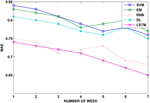
Figure 6. MAE for the weekly load estimations of power load using machine learning algorithms.

The SVM model achieved a 5.88% enhancement in prediction accuracy, indicating that its predictions were, on average, 5.88% closer to the actual values. Similarly, the EM model’s accuracy improved by approximately 4.88%, resulting in less deviation from the actual values. The RNN model notably enhanced its predictions, reducing the error by 6.10%. Likewise, the DL model showed an improvement of approximately 5.88% in its predictions. The LSTM consistently delivered accurate predictions with minimal error, making it a reliable choice for users seeking stable forecasts.

4.3.1.4 Mutual information

The results of the MI variation demonstrate that higher MI values correspond to better LSTM predictions, whereas SVM and EM exhibit lower MI values, indicating weaknesses compared to the RNN, DL, and LSTM. These findings collectively highlight a significant enhancement in the prediction accuracy of the LSTM method compared to other prediction models.

Over the course of 7 days, the SVM model exhibited a 12.5% improvement in performance. This enhancement translates to a significant increase in accuracy for SVM predictions. Similarly, the EM model showed an improvement of 10.3% in prediction accuracy. The RNN model notably enhanced its predictions by 8.8%. The DL model maintained consistent performance without any decrease. The LSTM consistently delivered reliable predictions with minimal deviation.

4.3.2 Monthly load forecast analysis

Throughout the monthly analysis, we adjusted the hyperparameter settings and conducted the same prediction tests over a 12-month period. Figures 8–11 show the load fitting curves for 12-month load predictions generated by various models. The LSTM model consistently reflects the actual load, while the curves for the SVM and EM models deviate significantly from the actual load, making them the least accurate among all the models. Importantly, the LSTM model proposed in this context shows the closest alignment with the actual load compared to other models.

4.3.2.1 Root mean squared error

Figure 8 shows the RMSE for the monthly load forecast, featuring machine learning algorithms including SVM, RNN, EM, DL, and LSTM. The SVM model’s predictions experienced a 7.69% improvement in terms of the RMSE. Similarly, the EM model’s accuracy was enhanced by 8.33%. The RNN model notably improved its predictions by 9.09%. Meanwhile, the DL model maintained steady performance without any deterioration, demonstrating consistent predictions. The RMSE value remained consistently low for LSTM, indicating its reliability and minimally varying predictions.

4.3.2.2 Normalized mean square error

Figure 9 gives the NMSE for the monthly forecast. Across all months, the LSTM model consistently demonstrates superior performance, exhibiting the lowest NMSE values. This consistency suggests that it is the most accurate model among those compared. Both the SVM and EM models show similar trends, with their NMSE values closely aligned, although SVM slightly outperforms EM. Similarly, the RNN and DL models exhibit comparable trends, with the RNN showing a slight edge over DL.

The SVM model starts with the highest NMSE but shows significant improvement over time, achieving a reduction of approximately 40% in the NMSE. Conversely, the ensemble classifier maintains consistent performance but does not demonstrate as much improvement as SVM, only reducing the NMSE by 15%. Initially, the deep learning model outperforms both EM and SVM models, but its improvement rate slows down, resulting in a reduction of approximately 25% in the NMSE.

The RNN model begins with a lower NMSE and steadily improves over time, achieving a 30% reduction in the NMSE. However, LSTM consistently maintains the best performance throughout, achieving a remarkable 50% reduction in the NMSE. Overall, LSTM emerges as the most consistent and effective model, achieving the highest reduction in the NMSE over the 12-month period.

4.3.2.3 Mean absolute error

In contrast, the RNN and DL models exhibit suboptimal performance across these metrics. Although the RNN model surpasses the DL, EM, and SVM models regarding the MAE, it does not match the performance of the LSTM and DL models in terms of the NMSE.

Consistently, SVM demonstrates the highest MAE across all months, suggesting that it may be the least accurate model in this context. On the contrary, LSTM exhibits a consistent decrease in the MAE from months 0 to 12, indicating an enhancement in accuracy over time. The EM and RNN models show similar patterns, with EM generally performing slightly better than the RNN. DL’s performance fluctuates but consistently remains lower than that of SVM and higher than that of LSTM. When considering overall performance, LSTM emerges as the best-performing model, followed by the DL, EM, and RNN models. SVM consistently falls behind the other models in terms of accuracy.

4.3.2.4 Mutual information

Figure 11 shows the mutual information for the monthly load forecast, displaying the performance of five machine learning models (SVM, EM, DL, RNN, and LSTM) across a span of 12 months.

The MI variation results show that higher MI values align with improved LSTM predictions, whereas SVM and EM present lower MI values, indicating relative weaknesses compared to the RNN, DL, and LSTM. The DL and RNN models outperform SVM and EM, showcasing a comparable range of predictions. Overall, these findings underscore a notable enhancement in the prediction accuracy of the LSTM method compared to other models. The RNN exhibits the most substantial improvement (4%), while the SVM experiences a slight decrease (2%).

5 Conclusion and future scope

The vitality of the energy industry hinges on the reliability of power demand forecasting. This study seeks to evaluate the precision of power consumption prediction using machine learning algorithms and hybrid models that incorporate artificial neural networks. Employing these advanced techniques has the potential to significantly improve power load forecasting performance. Several machine learning models are proposed in this study for short-term power load forecasting.

Unlike conventional statistical forecasting models, machine learning algorithms offer numerous advantages, including the effective management of nonlinear complexities and the ability to predict both short-term and long-term dependencies within power load time-series data. This study places emphasis on this crucial aspect. Analysis of the results shows that Figures 4–11 reveal that LSTM outperforms SVM, DL, EM, and RNN regression models in predicting electricity consumption. The approach involves using a sliding time window to convert multidimensional data into a continuous feature map input, harnessing the effectiveness of the CNN in spatial feature extraction. Our methodology is centered on a moving window-based LSTM network, enabling the prediction of demand for specific time intervals.

Figure 7

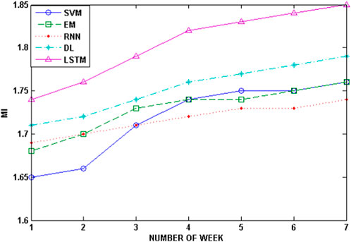
Figure 7. MI for the weekly load estimations of power load using machine learning algorithms.

Figure 8

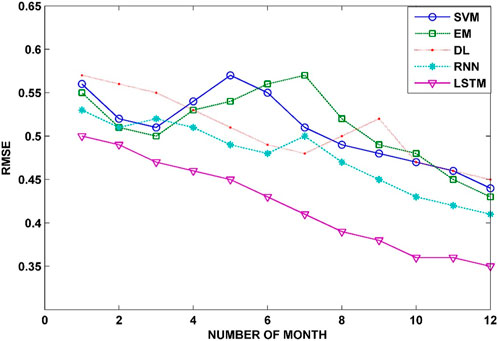
Figure 8. RMSE for the monthly power load estimations using machine learning algorithms.

Figure 9

Figure 9. NMSE for the monthly power load estimations.

Figure 10

Figure 10. MAE for the monthly power load estimations.

Figure 11

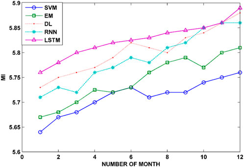
Figure 11. MI for the monthly power load estimations.

Following experimental verification analysis, it is concluded that the LSTM model exhibits notable enhancements in the MAE, RMSE, and NMSE compared to alternative time-series prediction models, including SVM, DL, EM, and RNN algorithms. Notably, LSTM outperforms the RNN, DL, EM, and SVM by reductions of 1.35%, 9.45%, 12.16%, and 13.51%, respectively, in predicting the load for the week.

Data availability statement

Publicly available datasets were analyzed in this study. These data can be found at: https://www.indiastat.com/chandigarh-state/data/power/power-demand-and-supply.

Author contributions

AJ: conceptualization, data curation, formal analysis, methodology, software, validation, writing–original draft, and writing–review and editing. SG: conceptualization, data curation, formal analysis, methodology, software, supervision, validation, writing–original draft, and writing–review and editing.

Funding

The author(s) declare that no financial support was received for the research, authorship, and/or publication of this article.

Conflict of interest

The authors declare that the research was conducted in the absence of any commercial or financial relationships that could be construed as a potential conflict of interest.

Publisher’s note

All claims expressed in this article are solely those of the authors and do not necessarily represent those of their affiliated organizations, or those of the publisher, the editors, and the reviewers. Any product that may be evaluated in this article, or claim that may be made by its manufacturer, is not guaranteed or endorsed by the publisher.

References

Ahmad, T., and Chen, H. (2019a). Deep learning for multi-scale smart energy forecasting. Energy 175, 98–112. doi:10.1016/j.energy.2019.03.080

CrossRef Full Text | Google Scholar

Ahmad, T., and Chen, H. (2019b). Nonlinear autoregressive and random forest approaches to forecasting electricity load for utility energy management systems. Sustain. Cities Soc. 45, 460–473. doi:10.1016/j.scs.2018.12.013

CrossRef Full Text | Google Scholar

Ahmad, T., and Chen, H. (2020). A review on machine learning forecasting growth trends and their real-time applications in different energy systems. Sustain. Cities Soc. 54, 102010. doi:10.1016/j.scs.2019.102010

CrossRef Full Text | Google Scholar

Ahmad, T., Huanxin, C., Zhang, D., and Zhang, H. (2020a). Smart energy forecasting strategy with four machine learning models for climate-sensitive and non-climate sensitive conditions. Energy 198, 117283. doi:10.1016/j.energy.2020.117283

CrossRef Full Text | Google Scholar

Ahmad, T., Zhang, H., and Yan, B. (2020b). A review on renewable energy and electricity requirement forecasting models for smart grid and buildings. Sustain. Cities Soc. 55, 102052. doi:10.1016/j.scs.2020.102052

CrossRef Full Text | Google Scholar

Ahmad, W., Ayub, N., Ali, T., Irfan, M., Awais, M., Shiraz, M., et al. (2020c). Towards short term electricity load forecasting using improved support vector machine and extreme learning machine. Energies 13, 2907. doi:10.3390/en13112907

CrossRef Full Text | Google Scholar

Ahmed, R., Sreeram, V., Mishra, Y., and Arif, M. D. (2020). A review and evaluation of the state-of-the-art in PV solar power forecasting: techniques and optimization. Renew. Sustain. Energy Rev. 124, 109792. doi:10.1016/j.rser.2020.109792

CrossRef Full Text | Google Scholar

Ahmed, S. F., Alam, M. S. B., Hassan, M., Rozbu, M. R., Ishtiak, T., Rafa, N., et al. (2023). Deep learning modelling techniques: current progress, applications, advantages, and challenges. Artif. Intell. Rev. 56, 13521–13617. doi:10.1007/s10462-023-10466-8

CrossRef Full Text | Google Scholar

Almaghrebi, A., Aljuheshi, F., Rafaie, M., James, K., and Alahmad, M. (2020). Data-driven charging demand prediction at public charging stations using supervised machine learning regression methods. Energies 13, 4231. doi:10.3390/en13164231

CrossRef Full Text | Google Scholar

Antonopoulos, I., Robu, V., Couraud, B., Kirli, D., Norbu, S., Kiprakis, A., et al. (2020). Artificial intelligence and machine learning approaches to energy demand-side response: a systematic review. Renew. Sustain. Energy Rev. 130, 109899. doi:10.1016/j.rser.2020.109899

CrossRef Full Text | Google Scholar

Aslam, S., Herodotou, H., Mohsin, N. S. M., Javaid, N., Ashraf, S., and Aslam, (2021). A survey on deep learning methods for power load and renewable energy forecasting in smart microgrids. Renew. Sustain. Energy Rev. 144, 110992. doi:10.1016/j.rser.2021.110992

CrossRef Full Text | Google Scholar

Bakay, M., Sevgül, Ü., and Ag˘bulut, (2021). Electricity production based forecasting of greenhouse gas emissions in Turkey with deep learning, support vector machine and artificial neural network algorithms. J. Clean. Prod. 285, 125324. doi:10.1016/j.jclepro.2020.125324

CrossRef Full Text | Google Scholar

Bedi, J., and Toshniwal, D. (2019). Deep learning framework to forecast electricity demand. Appl. energy 238, 1312–1326. doi:10.1016/j.apenergy.2019.01.113

CrossRef Full Text | Google Scholar

Caicedo-Vivas, J. S., and Alfonso-Morales, W. (2023). Short-term load forecasting using an LSTM neural network for a grid operator. Energies 16, 7878. doi:10.3390/en16237878

CrossRef Full Text | Google Scholar

Chammas, M., Makhoul, A., and Demerjian, J. (2019). An efficient data model for energy prediction using wireless sensors. Comput. Electr. Eng. 76, 249–257. doi:10.1016/j.compeleceng.2019.04.002

CrossRef Full Text | Google Scholar

Chapaloglou, S., Nesiadis, A., Iliadis, P., Atsonios, K., Nikolopoulos, N., Grammelis, P., et al. (2019). Smart energy management algorithm for load smoothing and peak shaving based on load forecasting of an island’s power system. Appl. energy 238, 627–642. doi:10.1016/j.apenergy.2019.01.102

CrossRef Full Text | Google Scholar

Chen, K., Chen, K., Wang, Q., and He, Z. (2018). Short-term load forecasting with deep residual networks. IEEE Trans. Smart Grid 99. doi:10.1109/TSG.2018.2844307

CrossRef Full Text | Google Scholar

Choi, E., Cho, S., and Kim, D. K. (2020). Power demand forecasting using long short-term memory (LSTM) deep-learning model for monitoring energy sustainability. Sustainability 12, 1109. doi:10.3390/su12031109

CrossRef Full Text | Google Scholar

Dinh, V., Phuong, V. V., Duong, M. Q., Kies, A., Schyska, B. U., and Wu, Y. K. (2018). “A short-term wind power forecasting tool for Vietnamese wind farms and electricity market,” in 4th International Conference on Green Technology and Sustainable Development (GTSD), Ho Chi Minh City, Vietnam, 130–135.

Google Scholar

El-Hendawi, M., and Wang, Z. (2020). An ensemble method of full wavelet packet transform and neural network for short term electrical load forecasting. Electr. Power Syst. Res. 182, 106265. doi:10.1016/j.epsr.2020.106265

CrossRef Full Text | Google Scholar

Fan, , Guo-Feng, Y.-H., Guo, J.-M., Zheng, W.-C., and Hong, (2019). Application of the weighted k-nearest neighbor algorithm for short-term load forecasting. Energies 12, 916. doi:10.3390/en12050916

CrossRef Full Text | Google Scholar

Fathi, S., Srinivasan, R., Fenner, A., and Fathi, S. (2020). Machine learning applications in urban building energy performance forecasting: a systematic review. Renew. Sustain. Energy Rev. 133, 110287. doi:10.1016/j.rser.2020.110287

CrossRef Full Text | Google Scholar

Gao, M., Li, J., Hong, F., and Long, D. (2019). Day-ahead power forecasting in a large-scale photovoltaic plant based on weather classification using LSTM. Energy 187, 115838. doi:10.1016/j.energy.2019.07.168

CrossRef Full Text | Google Scholar

Ghoddusi, , Hamed, G. G., Creamer, N., and Rafizadeh, (2019). Machine learning in energy economics and finance: a review. Energy Econ. 81, 709–727. doi:10.1016/j.eneco.2019.05.006

CrossRef Full Text | Google Scholar

Hao, Y., Dong, L., Liao, X., Liang, J., Wang, L., and Wang, B. (2019). A novel clustering algorithm based on mathematical morphology for wind power generation prediction. Renew. energy 136, 572–585. doi:10.1016/j.renene.2019.01.018

CrossRef Full Text | Google Scholar

Heydari, A., Nezhad, M. M., Pirshayan, E., Garcia, D. A., Keynia, F., and De Santoli, L. (2020). Short-term electricity price and load forecasting in isolated power grids based on composite neural network and gravitational search optimization algorithm. Appl. Energy 277, 115503. doi:10.1016/j.apenergy.2020.115503

CrossRef Full Text | Google Scholar

Hou, R., Li, S., Wu, M., Ren, G., Gao, W., Khayatnezhad, M., et al. (2021). Assessing of impact climate parameters on the gap between hydropower supply and electricity demand by RCPs scenarios and optimized ANN by the improved Pathfinder (IPF) algorithm. Energy 237, 121621. doi:10.1016/j.energy.2021.121621

CrossRef Full Text | Google Scholar

Hu, H., Wang, L., Peng, L., and Zeng, Y.-R. (2020). Effective energy consumption forecasting using enhanced bagged echo state network. Energy 193, 116778. doi:10.1016/j.energy.2019.116778

CrossRef Full Text | Google Scholar

Ibrahim, M., Sohail, W., Dong, Q., and Yang, (2020). Machine learning driven smart electric power systems: current trends and new perspectives. Appl. Energy 272, 115237. doi:10.1016/j.apenergy.2020.115237

CrossRef Full Text | Google Scholar

Jiang, P., Li, R., Liu, N., and Gao, Y. (2020). A novel composite electricity demand forecasting framework by data processing and optimized support vector machine. Appl. Energy 260, 114243. doi:10.1016/j.apenergy.2019.114243

CrossRef Full Text | Google Scholar

Jørgensen, K., Lau, H. R., and Shaker, (2020). “Wind power forecasting using machine learning: state of the art, trends and challenges,” in 2020 IEEE 8th International Conference on Smart Energy Grid Engineering (SEGE), Oshawa, ON, Canada, August, 2020, 44–50.

Google Scholar

Khan, P., Waqas, Y.-C., Byun, S.-J., Lee, D.-H., Kang, J.-Y., Kang, H.-S., et al. (2020a). Machine learning-based approach to predict energy consumption of renewable and nonrenewable power sources. Energies 13, 4870. doi:10.3390/en13184870

CrossRef Full Text | Google Scholar

Khan, W., Prince, Y.-C., Byun, S.-J., Lee, N., and Park, (2020b). Machine learning based hybrid system for imputation and efficient energy demand forecasting. Energies 13, 2681. doi:10.3390/en13112681

CrossRef Full Text | Google Scholar

Lai, J.-P., Chang, Y.-M., Chen, C.-H., and Pai, P.-F. (2020). A survey of machine learning models in renewable energy predictions. Appl. Sci. 10, 5975. doi:10.3390/app10175975

CrossRef Full Text | Google Scholar

Li, L.-L., Zhao, X., Tseng, M.-L., and Tan, R. R. (2020). Short-term wind power forecasting based on support vector machine with improved dragonfly algorithm. J. Clean. Prod. 242, 118447. doi:10.1016/j.jclepro.2019.118447

CrossRef Full Text | Google Scholar

Lu, R., Hong, S. H., and Yu, M. (2019). Demand response for home energy management using reinforcement learning and artificial neural network. IEEE Trans. Smart Grid 10, 6629–6639. doi:10.1109/tsg.2019.2909266

CrossRef Full Text | Google Scholar

Mosavi, A., Salimi, M., Ardabili, S. F., Rabczuk, T., Shamshirband, S., and Varkonyi-Koczy, A. R. (2019). State of the art of machine learning models in energy systems, a systematic review. Energies 12, 1301. doi:10.3390/en12071301

CrossRef Full Text | Google Scholar

O dwyer, E., Pan, I., Acha, S., and Shah, N. (2019). Smart energy systems for sustainable smart cities: current developments, trends and future directions. Appl. energy 237, 581–597. doi:10.1016/j.apenergy.2019.01.024

CrossRef Full Text | Google Scholar

Pawar, P., Tarunkumar, M., and Vittal K., P. (2020). An IoT based Intelligent Smart Energy Management System with accurate forecasting and load strategy for renewable generation. Measurement 152, 107187. doi:10.1016/j.measurement.2019.107187

CrossRef Full Text | Google Scholar

Prado, , Francisco, M. C., Minutolo, W., and Kristjanpoller, (2020). Forecasting based on an ensemble autoregressive moving average-adaptive neuro-fuzzy inference system-neural network-genetic algorithm framework. Energy 197, 117159. doi:10.1016/j.energy.2020.117159

CrossRef Full Text | Google Scholar

Qiao, W., Lu, H., Zhou, G., Azimi, M., Yang, Q., and Tian, W. (2020). A hybrid algorithm for carbon dioxide emissions forecasting based on improved lion swarm optimizer. J. Clean. Prod. 244, 118612. doi:10.1016/j.jclepro.2019.118612

CrossRef Full Text | Google Scholar

Reynolds, J., Ahmad, M. W., Rezgui, Y., and Hippolyte, J.-L. (2019). Operational supply and demand optimisation of a multi-vector district energy system using artificial neural networks and a genetic algorithm. Appl. energy 235, 699–713. doi:10.1016/j.apenergy.2018.11.001

CrossRef Full Text | Google Scholar

Santamouris, M. (2020). Recent progress on urban overheating and heat island research. Integrated assessment of the energy, environmental, vulnerability and health impact. Synergies with the global climate change. Energy Build. 207, 109482. doi:10.1016/j.enbuild.2019.109482

CrossRef Full Text | Google Scholar

Satre-Meloy, A. M., Diakonova, P., and Grünewald, (2020). Cluster analysis and prediction of residential peak demand profiles using occupant activity data. Appl. Energy 260, 114246. doi:10.1016/j.apenergy.2019.114246

CrossRef Full Text | Google Scholar

Shaw, R., Howley, E., and Barrett, E. (2019). An energy efficient anti-correlated virtual machine placement algorithm using resource usage predictions. Simul. Model. Pract. Theory 93, 322–342. doi:10.1016/j.simpat.2018.09.019

CrossRef Full Text | Google Scholar

Skala, R., Elgalhud, M. A. T. A., Grolinger, K., and Mir, S. (2023). Interval load forecasting for individual households in the presence of electric vehicle charging. Energies 16, 4093. doi:10.3390/en16104093

CrossRef Full Text | Google Scholar

Somu, N., Raman, G., R, M., and Ramamritham, K. (2021). A deep learning framework for building energy consumption forecast. Renew. Sustain. Energy Rev. 137, 110591. doi:10.1016/j.rser.2020.110591

CrossRef Full Text | Google Scholar

Su, M., Zhang, Z., Zhu, Y., Zha, D., and Wen, W. (2019). Data driven natural gas spot price prediction models using machine learning methods. Energies 12, 1680. doi:10.3390/en12091680

CrossRef Full Text | Google Scholar

Sun, Y., Haghighat, F., Benjamin, , and Fung, (2020). A review of the-state-of-the-art in data-driven approaches for building energy prediction. Energy Build. 221, 110022. doi:10.1016/j.enbuild.2020.110022

CrossRef Full Text | Google Scholar

Ullah, Z., Al-Turjman, F., Mostarda, L., and Gagliardi, R. (2020). Applications of artificial intelligence and machine learning in smart cities. Comput. Commun. 154, 313–323. doi:10.1016/j.comcom.2020.02.069

CrossRef Full Text | Google Scholar

ur Rehman Khan, S., Hayder, I. A., Habib, M. A., Ahmad, M., Mohsin, S. M., Khan, F. A., et al. (2023). Enhanced machine-learning techniques for medium-term and short-term electric-load forecasting in smart grids. Energies 16, 276. doi:10.3390/en16010276

CrossRef Full Text | Google Scholar

Walker, S., Khan, W., Katic, K., Maassen, W., and Zeiler, W. (2020). Accuracy of different machine learning algorithms and added-value of predicting aggregated-level energy performance of commercial buildings. Energy Build. 209, 109705. doi:10.1016/j.enbuild.2019.109705

CrossRef Full Text | Google Scholar

Wang, H., Lei, Z., Zhang, X., Zhou, B., and Peng, J. (2019). A review of deep learning for renewable energy forecasting. Energy Convers. Manag. 198, 111799. doi:10.1016/j.enconman.2019.111799

CrossRef Full Text | Google Scholar

Wang, H., Liu, Y., Zhou, B., Li, C., Cao, G., Voropai, N., et al. (2020a). Taxonomy research of artificial intelligence for deterministic solar power forecasting. Energy Convers. Manag. 214, 112909. doi:10.1016/j.enconman.2020.112909

CrossRef Full Text | Google Scholar

Wang, R., Lu, S., and Feng, W. (2020b). A novel improved model for building energy consumption prediction based on model integration. Appl. Energy 262, 114561. doi:10.1016/j.apenergy.2020.114561

CrossRef Full Text | Google Scholar

Xue, P., Jiang, Y., Zhou, Z., Chen, X., Fang, X., and Liu, J. (2019). Multi-step ahead forecasting of heat load in district heating systems using machine learning algorithms. Energy 188, 116085. doi:10.1016/j.energy.2019.116085

CrossRef Full Text | Google Scholar

Zhang, L., Wen, J., Li, Y., Chen, J., Ye, Y., Fu, Y., et al. (2021). A review of machine learning in building load prediction. Appl. Energy 285, 116452. doi:10.1016/j.apenergy.2021.116452

CrossRef Full Text | Google Scholar

Zheng, X., Yang, M., Yu, Y., and Wang, C. (2023). Short-term net load forecasting for regions with distributed photovoltaic systems based on feature reconstruction. Appl. Sci. 13, 9064. doi:10.3390/app13169064

CrossRef Full Text | Google Scholar

Zhou, Y., Ravey, A., and Péra, M.-C. (2019). A survey on driving prediction techniques for predictive energy management of plug-in hybrid electric vehicles. J. Power Sources 412, 480–495. doi:10.1016/j.jpowsour.2018.11.085

CrossRef Full Text | Google Scholar