Study on the prediction method of ceasing–flowing for self-flowing wells

Currently, most of the wells in X Oilfield are self-flowing wells. In order to adjust the production system of oil wells in time according to the production requirements of oilfields, it is necessary to predict the ceasing–flowing time. Therefore, how to accurately predict the ceasing–flowing time is the main problem faced by the self-flowing well. As the conventional prediction methods only consider the influence of a single variable, the prediction results are not ideal. Combining the production prediction based on the long short-term memory (LSTM) neural network and the inflow and outflow dynamic curves, this study proposes a comprehensive method for predicting the ceasing–flowing time of a flowing well by considering multiple factors. Using the minimum wellhead pressure prediction method, the changes in bottom hole flowing pressure and reservoir pressure are also considered. The practical application results in X Oilfield show that the calculated and predicted results are highly consistent with the actual production data, verifying the reliability of this method. This study can provide a reference for the prediction of oil well ceasing–flowing in other oilfields.

1 Introduction

The bottom hole flowing pressure and reservoir pressure are the basis for analyzing the production performance of the oil wells and are also important parameters that affect the production capacity and adjustment scheme of the oilfield. The determination of the bottom hole flowing pressure and reservoir pressure is a prerequisite for the stable and high production of the oil well. Currently, the main ways to obtain the bottom hole flowing pressure are instrument measurement and calculation methods. Ye et al. studied the relationship between fluid density and pressure drop gradient under different flow conditions based on the liquid level folding algorithm and applied the calculus method to calculate the bottom hole flowing pressure (Ye et al., 2017).

Due to the significant impact of factors such as pipeline size and fluid properties on pressure decrease, it is difficult to establish a unified model that comprehensively considers various flow conditions to calculate the wellbore pressure gradient. The existing models are mainly divided into two categories, namely, empirical models and mechanism models. Duns and Ros, Hagedorn and Brown, Orkiszewski, Beggs, and Brill, and Mukherjee and Brill are empirical models, while Aziz, Ansari, and Hasan are mechanism models (Duns and Ros, 1963; Brill et al., 1966; Orkiszewski, 1967; Aziz et al., 1972; Beggs and Brill, 1973; Mukherjee and Brill, 1983; Hasan and Kabir, 1988; Ansari et al., 1994). Through comprehensive research and comparisons with the previously mentioned methods, the Beggs and Brill method is widely applicable to vertical, inclined, and horizontal wells. In addition, the theory of the Beggs and Brill method is mature and convenient for programming and debugging. Therefore, in this study, the Beggs and Brill model was selected to fit the pressure and temperature of the wellbore profile and then combined with the Bayesian automatic algorithm to calculate the bottom hole flowing pressure.

Currently, scholars mainly use the following methods to calculate reservoir pressure: 1) directly obtaining reservoir pressure through pressure recovery testing and well shut-in pressure measurement, but the pressure recovery time is long, making it difficult to test each well (Chen et al., 2017); 2) the wellhead pressure reduction algorithm, but the establishment of empirical formulas requires a large amount of testing data (Zhang et al., 2021); 3) the theoretical formula method, which uses the production capacity equation, requires the production capacity equation to be accurate and the pressure and production at the wellhead to be relatively stable (Yang and Cun, 2009); and 4) the material balance method, which was chosen in this study to calculate reservoir pressure as it can accurately calculate reservoir pressure and is not limited by factors such as data completeness and applicability (Wu et al., 2022).

Considering the time characteristics of oil well production data, it is necessary to use a time-series model for predicting production and pressure. Currently, time-series models have made significant progress in the field of artificial intelligence and are successfully applied in the dynamic prediction of oil and gas well production (Frausto-Solís et al., 2015). These prediction models improve universality as they only consider historical data. This study selects a deep learning algorithm suitable for time-series analysis based on the decline curve of oil well production.

Because the BP neural network shows a large deviation in prediction results, scholars put forward the concept of a recurrent neural network (RNN) to try to enhance the grasp of the timing of information (David et al., 1986; Elman, 1990). However, the RNN is difficult to be used for practical operations because the system will be unstable with time. Therefore, Hochreiter and Schmidhuber proposed the long short-term memory (LSTM) neural network method, which is a variant of the RNN (Hochreiter and Schmidhuber, 1997). To solve the problem of the RNN model, researchers introduced unit states and three control gates. The main goal of LSTM is to address long-term dependencies between data and iteratively transmit the impact between each level of data. Unit states were used to determine information retention between different time steps, and control gates were set to adjust the information transfer function between different positions (Xue et al., 2023). The modified neural network structure is shown in Figure 1.

Figure 1

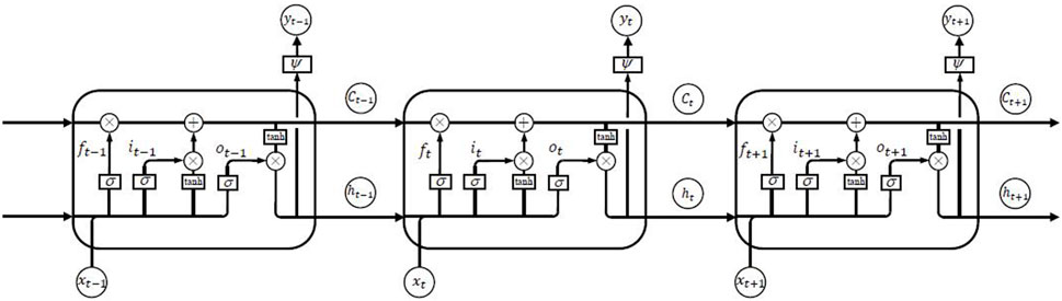
Figure 1. Long short-term memory (LSTM) neural network structure (Xue et al., 2023).

There is a phenomenon of production decrease in actual oil well production, but traditional neural network methods only train the original dataset for calculation and do not consider this factor. Therefore, in the process of yield prediction, it is necessary to introduce a suitable prediction model and combine it with neural network methods to improve the training performance of the neural network. In recent years, scholars have proposed many prediction models for production prediction. The decline curves analysis (DCA) model has the advantages of simplicity and efficiency and is widely used in the prediction of oil and natural gas production. Song et al. proposed a model based on the LSTM neural network to address the limitations of traditional methods in time-series production rate prediction, taking production constraints into account (Song et al., 2020). Li et al. developed a deep learning model based on the LSTM neural network model that can consider the influence of manual operations. This model can predict the ceasing–flowing time, choke size, and oil well production rate (Li et al., 2022).

The oil wells in X Oilfield are mostly self-flowing wells, and to adjust production systems on time, accurate prediction of ceasing–flowing of oil wells is necessary. The conventional methods for predicting the ceasing–flowing time mainly include 1) calculating the ceasing–flowing pressure through a formula and predicting future flow pressure changes. The corresponding time when the flow pressure reaches the ceasing–flowing pressure is the ceasing–flowing time (Yang et al., 2014); 2) determining the minimum wellhead pressure and regressing the trend of oil pressure changes; 3) calculating the minimum bottom hole flowing pressure and predicting changes in bottom hole flowing pressure; and 4) calculating the minimum reservoir pressure and regressing the trend of reservoir pressure changes (Wang et al., 2014). However, the aforementioned methods only consider a single factor when predicting the ceasing–flowing time, and the accuracy of the prediction results is poor. Therefore, this study proposed a comprehensive method that considers multiple factors to predict the ceasing–flowing time of a flowing well, taking into account both changes in flow pressure and reservoir pressure based on the minimum wellhead pressure prediction method. First, a suitable multiphase pipe flow model was selected based on data such as fluid pressure testing and production performance and fitted with the flow pressure and reservoir pressure using the Bayesian algorithm and material balance method. Furthermore, the LSTM neural network algorithm driven by the DCA model was used to predict the production, pressure, and oil-recovery index. Then, based on the predicted production, the predicted inflow performance relationship (IPR) and wellhead performance relationship (WPR) curves were drawn to determine the minimum wellhead pressure for the well to ceasing–flowing. Finally, the warning level for each well can be determined by the difference between the current and minimum wellhead pressure. This method fully considers the current development status of X Oilfield, and the prediction results were relatively accurate, which can provide a technical reference for the analysis and research of stopping flow prediction in flowing wells.

2 Calculation of bottom hole flowing pressure and reservoir pressure

2.1 Bottom hole flowing pressure calculation

As shown in Figure 2, to further verify the applicability of the Beggs and Brill method in X Oilfield, the fitting results of different bottom hole flowing pressures and test pressure profiles for A-well were compared. The comparison results show that the Beggs and Brill method has extremely high fitting accuracy.

Figure 2

Figure 2. Fitting results of pressure profiles of A-well.

Based on the Beggs and Brill method, this study used the Python platform for programming the calculation of bottom hole flowing pressure and developed modules for basic parameters, physical parameter calculation, temperature calculation, pressure loss calculation, and pressure and temperature gradient calculation. Moreover, to improve the fitting accuracy of the test profile data and reduce human interference, the Bayesian optimization algorithm was further combined to realize the automatic fitting and optimization of the uncertain sequence array.

Based on the bottom hole flowing pressure obtained by the Beggs and Brill model, the automatic bottom hole flowing pressure fitting was carried out in combination with the Bayesian optimization algorithm. The process of automatic bottom hole flowing pressure fitting is shown in Figure 3. First, the unit is normalized based on pressure, density, and temperature profile data, and the search space is defined based on basic parameters such as GOR. Then, when the iteration times (N) is less than the maximum limit, the profile and normalized mean squared error (MSE) loss were calculated compared to the test data, which is a multi-target optimization process. Next, acquisition function (AF) was updated, and a new hyperparameter was acquired. Finally, the aforementioned process was repeated until the loss converges.

Figure 3

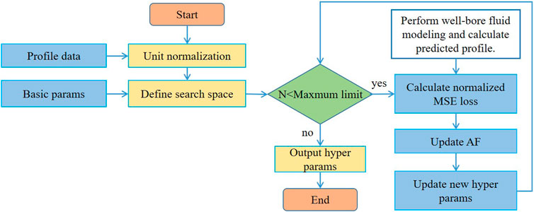
Figure 3. Process of automatic bottom hole flowing pressure fitting.

Using the Bayesian optimization algorithm, the uncertainty parameters were taken as optimization variables, and the average error between the calculated pressure profile and measured pressure profile and between the calculated temperature and measured temperature of the reservoir was minimized as an optimization objective. Test data were added to iterative optimization to complete profile fitting, and the average fitting error was less than 5%. The average fitting time was 5–7 min, which greatly improves the efficiency and accuracy of pressure profile fitting. As shown in Table 1, the range of variation was set for each parameter, and the change in each parameter with production time is shown in Figure 4. Most parameters change with the change in bottom hole flowing pressure, but the amplitude of the change in each parameter was significantly different. The changes in water cut and gas relative density were significant, while saturation pressure and temperature gradient remained constant.

Table 1

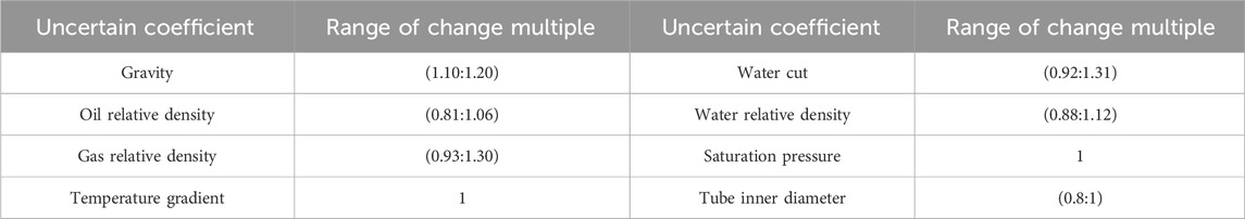
Table 1. Change ranges of uncertainty coefficients.

Figure 4

Figure 4. Automatic fitting result of uncertain coefficients.

2.2 Reservoir pressure calculation

Based on the accurate acquisition of bottom hole flowing pressure data, further research and calculation of producer inflow dynamics are necessary to accurately assess whether the producers are naturally flowing. To obtain the inflow performance characteristics of producers at a certain time, the first step is to predict the reservoir pressure at that time. In this study, the reservoir pressure was calculated based on the material balance method, i.e., the oil well and its drainage area are regarded as closed reservoir units, and the oil–water two-phase and oil–gas–water three-phase reservoir pressure prediction models were established. Combined with the least square method and Newton’s iterative method, the reservoir pressure at different times was calculated according to the relationship between cumulative production and reservoir pressure decrease.

The principle of material balance is as follows (Li, 2011):

$\begin{array}{l}{N}_{\mathrm{p}}\left[B_{\mathrm{o}}+\left(R_{\mathrm{p}}-R_{\mathrm{s}}\right)B_{\mathrm{g}}\right]+W_{\mathrm{p}}{B}_{\mathrm{w}}-W_{\mathrm{i}}{B}_{\mathrm{w}}-G_{\mathrm{i}}{B}_{\mathrm{g}}=\\ N\left[\left(B_{\mathrm{o}}-B_{\text{oi}}\right)+\left(R_{\text{si}}-R_{\mathrm{s}}\right)B_{\mathrm{g}}+\left(1+m\right)B_{\text{oi}}\frac{\left(C_{\mathrm{f}}+S_{\text{wc}}{C}_{\mathrm{w}}\right)}{\left(1-S_{\text{wc}}\right)}\Delta P+m{B}_{\text{oi}}\left(\frac{B_{\mathrm{g}}}{B_{\text{gi}}}-1\right)\right]+W_{\mathrm{e}},\end{array}$

where $B_{\mathrm{o}}+\left(R_{\mathrm{p}}-R_{\mathrm{s}}\right)B_{\mathrm{g}}$ is oil and dissolved gas production, $W_{\mathrm{p}}{B}_{\mathrm{w}}$ is water production, $W_{\mathrm{i}}{B}_{\mathrm{w}}$ is water injection, $G_{\mathrm{i}}{B}_{\mathrm{g}}$ is gas injection, $\left(B_{\mathrm{o}}-B_{\text{oi}}\right)+\left(R_{\text{si}}-R_{\mathrm{s}}\right)B_{\mathrm{g}}$ is oil and dissolved gas expansion, $\left(1+m\right)B_{\text{oi}}\frac{\left(C_{\mathrm{f}}+S_{\text{wc}}{C}_{\mathrm{w}}\right)}{\left(1-S_{\text{wc}}\right)}\Delta P$ is the compression of pore space and connate water expansion, $m{B}_{\text{oi}}\left(\frac{B_{\mathrm{g}}}{B_{\text{gi}}}-1\right)$ is gas cap expansion, and $W_{\mathrm{e}}$ is water influx.

Using the aforementioned method, this study compared the calculated reservoir pressure and measured reservoir pressure of each well in different layers, and the results show that the aforementioned method can be used to calculate reservoir pressure with certain accuracy.

2.3 Bottom hole flowing pressure and reservoir pressure calculation result

The aforementioned method was used to calculate the daily bottom hole flowing pressure and reservoir pressure of each well. The calculated pressure was fitted with the measured pressure. According to the fitting results of reservoir pressure and bottom hole flowing pressure, the time-series curves of reservoir pressure and bottom hole flowing pressure in different production dates were drawn, as shown in Figure 5. In general, the fitting results were good, and the time sequence bottom hole flowing pressure and reservoir pressure calculated by each well have a high accuracy. The aforementioned theory and method can be used to calculate the bottom hole flowing pressure and reservoir pressure.

Figure 5

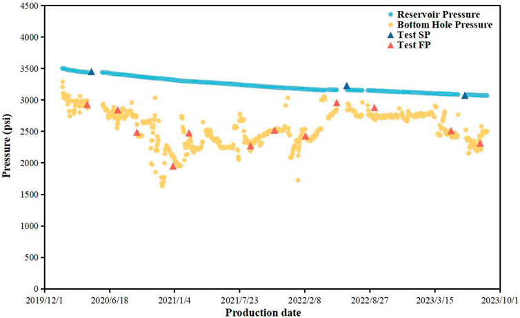
Figure 5. Bottom hole flowing pressure and reservoir pressure calculation results of A-well.

3 Production prediction based on the LSTM neural network and DCA model

Based on the historical production data such as oil production rate, gas production rate, and wellhead pressure, we used the LSTM neural network model constrained by the DCA production decline model to predict the production and pressure. The dynamic curves of inflow and outflow were drawn, and then the curves of the coordination point change were obtained.

3.1 LSTM neural network

Each cell state is composed of three multiplicative gating connections, namely, input gate (i_t), forget gate (f_t), and output gate (o_t). The function of each gate can be interpreted as write, reset, and read operations, concerning the internal cell state. The gates in a memory cell facilitate keeping and accessing the internal cell states over long periods. The LSTM output would depend on all previous inputs. Previous information is neither completely discarded nor completely carried over to the current state. Instead, the influence of the previous information on the current state is carefully controlled through the gate signals.

The forget gate f_t at time t is calculated as follows (Xue et al., 2023):

$f_t=\sigma \left(W_f{x}_t+U_f{h}_{t-1}+b_f\right),$

where $\sigma$ represents the sigmoid function; $W_f$ and $U_f$ are the weight parameters; $b_f$ represents the bias of the forget gate; and $h_{t-1}$ is the output information of the hidden layer.

The input gate i_t at time t can be expressed as follows:

$i_t=\sigma \left(W_i{x}_t+U_i{h}_{t-1}+b_i\right),$

where $W_i$ and $U_i$ are the weight parameters and $b_i$ represents the bias of the input gate. It outputs a value to send unit status information. Simultaneously, it can be determined which information from the previous unit status should be retained or discarded.

The candidate unit status C_t at time t can be calculated as follows:

$C_t=\tanh \left(W_c{x}_t+U_c{h}_{t-1}+b_c\right),$

where tanh represents the hyperbolic tangent activation function; $W_c$ and $U_c$ are the weight parameters of the LSTM cell; and $b_c$ represents the bias of the input gate.

The output gate o_t at time t is calculated as follows:

$o_t=\sigma \left(W_o{x}_t+U_o{h}_{t-1}+b_o\right),$

where $W_o$ and $U_o$ are the weight parameters and $b_o$ is the bias of the output gate.

The cell state can be expressed as follows:

$h_t=o_t\tanh \left(C_t\right).$

The aforementioned equations summarize formulas for the LSTM network forward pass. In an LSTM cell, activation functions are point-wise nonlinear functions that are typically logistic sigmoids for the gates and hyperbolic tangent (tanh) for input to and output from a node. In the full-precision LSTM, the lengths of all vectors are considered to be 32 bits.

3.2 Production forecasting jointly driven by the DCA model and data

The decline curve model can provide theoretical and empirical validation for the study of dynamic characteristics of oil production, and this validation information can serve as a reasonable constraint in the calculation process of neural network models (Xue et al., 2023). In this way, based on the actual historical production performance data of oil wells in the oilfield, the production performance data are organized into a time-series dataset. The LSTM neural network method driven by the DCA model is used to find and extract the internal relationship between the segments of the dataset and then predict the future production characteristics of the oil wells. A neural network model is established and trained, as shown in Figure 6. By combining the DCA model, the neural network training process can converge to its optimal state more quickly and accurately, improving the accuracy of its prediction results.

Figure 6

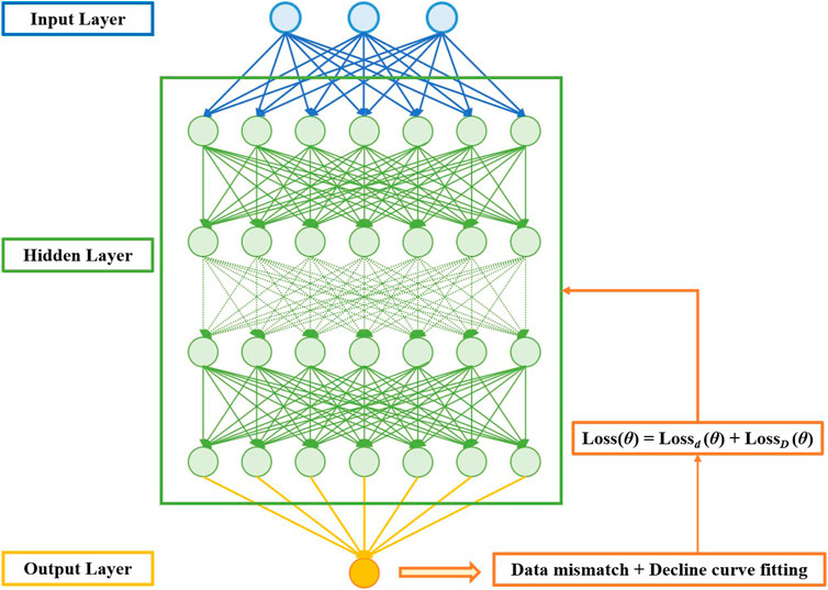
Figure 6. LSTM neural network method combined with the DCA model (Xue et al., 2023).

The DCA empirical model only needs to calibrate parameters based on the production data. Before combining the DCA model with the LSTM neural network model, it is necessary to select a suitable DCA model. Due to the complexity of fluid flow patterns, the ARPS model is not suitable for unconventional reservoirs (Arps, 1945; Nelson, 2009). For this reason, later scholars proposed models such as the stretched exponential decline model (SEPD) and the Duong model (Valkó and Lee, 2010; Duong, 2011). The calculation formula for the DCA model is as follows:

The ARPS model:

$q\left(t\right)=q_i{e}^{-D_{i}t},$

$q\left(t\right)=q_i{\left(1+b{D}_{i}t\right)}^{-1/b},$

$q\left(t\right)=q_i{\left(1+D{}_{i}t\right)}^{-1}.$

The stretched exponential decline model:

$q=q_i\exp \left[-{\left(t/\tau \right)}^{n_{\text{SEPD}}}\right].$

The Duong model:

$q=q_i{t}^{-m_D}\exp \left[a_D\left(t^{1-m_D}-1\right)/\left(1-m_D\right)\right].$

These five models are fitted to the training and testing datasets and are based on the fitting performance of these five DCA models. Then, the optimal model is selected and incorporated as a driving condition into the neural network.

3.3 Production and pressure prediction result

We predicted the future oil production index by fitting the recent oil production index changes. Based on the LSTM neural network machine learning model and DCA model, the oil production rate, gas production rate, and wellhead pressure were predicted. The production prediction results are shown in Figure 7A, and the wellhead pressure prediction result is shown in Figure 7B. Finally, the changes in coordination points were achieved, as shown in Figure 7C. It can be seen that the LSTM machine learning prediction results based on the production decline model have a good fitting effect with the historical production data. According to the predicted IPR and WPR curves, the minimum wellhead pressure can be determined when the oil well is ceasing–flowing. Then, the subsequent method was used to predict the ceasing–flowing time of oil wells.

Figure 7

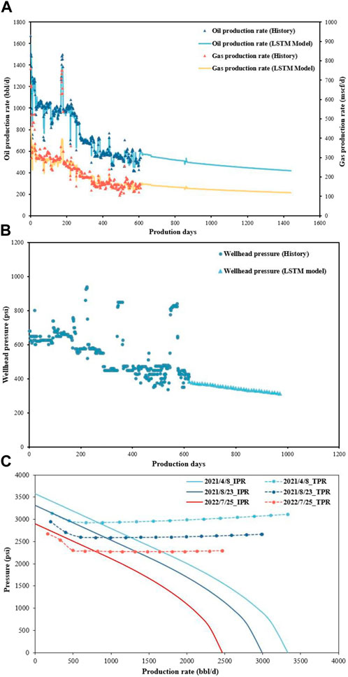
Figure 7. Dynamic indicator prediction results of A-well: (A) predicted results of the oil and gas production rate; (B) predicted results of wellhead pressure; and (C) time-series curves of IPR and WPR.

4 Minimum wellhead pressure ceasing–flowing warning model based on nodal analysis

X Oilfield is in the early stages of development, and most of the oil wells are produced by self-flowing. As production progresses, the reservoir pressure continues to decrease, and some oil wells gradually produce water. More and more oil wells are facing ceasing–flowing. To timely grasp the production situation of oil wells and adjust production systems, it is necessary to accurately predict the ceasing–flowing of oil wells. In this study, the minimum wellhead pressure method was selected for predicting the ceasing–flowing of oil wells.

As shown in Figure 8, the main steps of the minimum wellhead pressure ceasing–flowing warning are summarized as follows (Li, 2009): first, the future production rate and cumulative production are obtained by the LSTM network method. Then, by combining the reservoir pressure prediction method given in Section 2.2, the bottom hole pressure at that production rate can be obtained by drawing IPR curves, and the corresponding wellhead pressure value can be obtained by using the wellbore pressure calculation method. The yellow lines in the figure are the wellhead pressure curves (WPR) predicted by different production rates at a certain time in the future. When the curve intersects with the green line of the minimum wellhead pressure, it indicates that the oil well will not be able to self-flow after this moment. Thus, the difference between the current wellhead pressure and the minimum wellhead pressure can be used as a judgment for a ceasing–flowing warning.

Figure 8

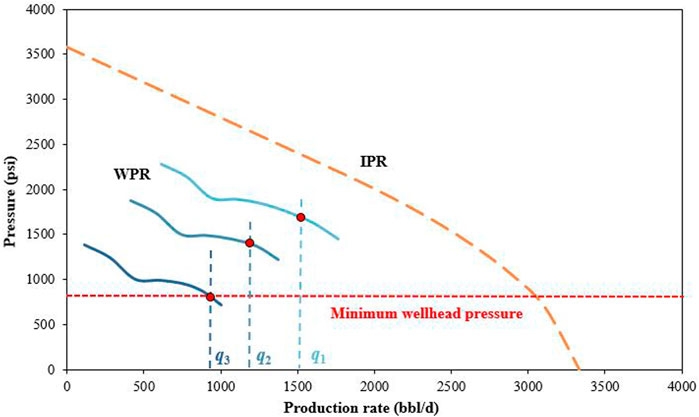
Figure 8. Ceasing–flowing warning using the minimum wellhead pressure method.

In addition, this project selected C-well as a representative well and applied the minimum pressure warning method based on the LSTM network method to carry out production performance prediction, as shown in Figure 9. We obtained the daily and cumulative production change curves given in Figure 9A for the next 1 year according to the LSTM. In addition, the daily and cumulative production change curves were combined with the material balance method to obtain the corresponding time-series IPR curves in Figure 9B and the predicted value of bottom hole flowing pressure and wellhead pressure in Figure 9C for the next 1 year. When the downstream pressure of the nozzle decreases to the minimum external pressure required for the wellhead, the oil well stops flowing. According to the predicted IPR and WPR curves, the minimum wellhead pressure of ceasing–flowing is determined. Therefore, the triggering condition is set to whether the wellhead pressure decreased to 300 psi.

Figure 9

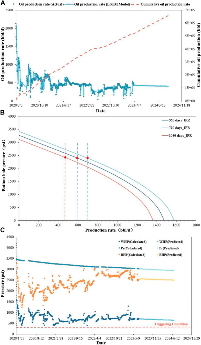
Figure 9. Production performance prediction results of B-well based on the minimum wellhead pressure warning method: (A) production rate and cumulative production change; (B) time-series IPR curves (the production rate value at the red dot in the figure represents the production rate corresponding to the production days); and (C) wellhead pressure and triggering condition.

5 Conclusion

1. The wellbore flow model based on the Beggs and Brill method was established, and by defining the uncertain parameter group and combining it with Bayesian automatic fitting, high-precision calculation results of bottom hole flowing pressure were obtained. Based on the principle of material balance, the reservoir pressure of each well was fitted, and the fitting results demonstrate the rationality of this method.

2. Based on the inflow and outflow dynamic curves, a comprehensive method for predicting the ceasing–flowing time of oil wells is proposed, which considers multiple factors. Based on the minimum wellhead pressure prediction method, the changes in flow pressure and reservoir pressure are also considered. The results provide a reference for predicting the ceasing–flowing time of self-flowing wells in other similar reservoirs.

3. Based on the LSTM machine learning method and using empirical production decline models for constraints, the prediction results of daily oil production, water production, and daily gas production in the next year were obtained. The prediction results provide a basis for the selection of artificial lifting time, ensuring the stable and efficient development of X Oilfield.

Data availability statement

The original contributions presented in the study are included in the article/Supplementary Material; further inquiries can be directed to the corresponding author.

Author contributions

BK: conceptualization, investigation, and writing–original draft. ZM: data curation, resources, and writing–original draft. YH: formal analysis, investigation, and writing–review and editing. LZ: project administration, software, and writing–original draft. RZ: methodology and writing–review and editing.

Funding

The authors declare that financial support was received for the research, authorship, and/or publication of this article. This work was supported by the National Natural Science Foundation of China (Grant No. 52304048) and the Sichuan Science and Technology Program (No. 2022JDJQ0009).

Acknowledgments

The authors acknowledge the National Natural Science Foundation of China (Grant No. 52304048) and the Sichuan Science and Technology Program (No. 2022JDJQ0009).

Conflict of interest

Authors BK, ZM, and LZ were employed by Chengdu North Petroleum Exploration and Development Technology Company Limited.

The remaining authors declare that the research was conducted in the absence of any commercial or financial relationships that could be construed as a potential conflict of interest.

The reviewer SS declared a shared affiliation with the authors, YH and RZ, to the handling editor at the time of review.

Publisher’s note

All claims expressed in this article are solely those of the authors and do not necessarily represent those of their affiliated organizations, or those of the publisher, the editors, and the reviewers. Any product that may be evaluated in this article, or claim that may be made by its manufacturer, is not guaranteed or endorsed by the publisher.

References

Ansari, A. M., Sylvester, N. D., Sarica, C., Shoham, O., and Brill, J. P. (1994). A comprehensive mechanistic model for upward two-phase flow in wellbores. SPE Prod. Facil. 9 (2), 143–151. doi:10.2118/20630-pa

CrossRef Full Text | Google Scholar

Arps, J. J. (1945). Analysis of decline curves. Trans. AIME 160 (1), 228–247. doi:10.2118/945228-g

CrossRef Full Text | Google Scholar

Aziz, K., Govier, G. W., and Fogarasi, M. (1972). Pressure drop in wells producing oil and gas. J. Can. Petroleum Technol. 11 (3), 38–47. doi:10.2118/72-03-04

CrossRef Full Text | Google Scholar

Beggs, H. D., and Brill, J. P. (1973). A study of two-phase flow in inclined pipes. J. Petroleum Technol. 25 (5), 607–617. doi:10.2118/4007-pa

CrossRef Full Text | Google Scholar

Brill, J. P., Doerr, T. C., Hagedorn, A. R., and Brown, K. E. (1966). Practical use of recent research in multi-phase vertical and horizontal flow. J. Petroleum Technol. 18 (4), 502–512. doi:10.2118/1245-pa

CrossRef Full Text | Google Scholar

Chen, X., Yu, Z. H., Luo, J. N., Gu, X. D., and Yue, J. (2017). The evaluation of present reservoir pressure of Sulige gas-field T2 block. Petrochem. Ind. Appl. 36 (11), 23–27. doi:10.3969/j.issn.1673-5285.2017.11.006

CrossRef Full Text | Google Scholar

David, E. R., Geoffrey, E. H., and Ronald, J. W. (1986). Learning representations by back-propagating errors. Nature 323, 533–536. doi:10.1038/323533a0

CrossRef Full Text | Google Scholar

Duns, H., and Ros, N. C. J. (1963). “Vertical flow of gas and liquid mixtures in wells,” in Sixth world Petroleum congress (Frankfurt am Main, Germany: One Petro). 19-26 June.

Google Scholar

Duong, A. N. (2011). Rate-decline analysis for fracture-dominated shale reservoirs. SPE Reserv. Eval. Eng. 14 (3), 377–387. doi:10.2118/137748-pa

CrossRef Full Text | Google Scholar

Elman, J. L. (1990). Finding structure in time. Cognitive Sci. 149 (2), 179–211. doi:10.1016/0364-0213(90)90002-e

CrossRef Full Text | Google Scholar

Frausto-Solís, J., Chi-Chim, M., and Sheremetov, L. (2015). Forecasting oil production time series with a population-based simulated annealing method. Arabian J. Sci. Eng. 40 (4), 1081–1096. doi:10.1007/s13369-015-1587-z

CrossRef Full Text | Google Scholar

Hasan, A. R., and Kabir, C. S. (1988). A study of multiphase flow behavior in vertical wells. SPE Prod. Eng. 3 (2), 263–272. doi:10.2118/15138-pa

CrossRef Full Text | Google Scholar

Hochreiter, S., and Schmidhuber, J. (1997). Long short-term memory. Neural Compute 9 (8), 1735–1780. doi:10.1162/neco.1997.9.8.1735

PubMed Abstract | CrossRef Full Text | Google Scholar

Li, C. L. (2011) Fundamentals of reservoir engineering. Beijing: Petroleum Industry Publishing House.

Google Scholar

Li, X., Xiao, K., Li, X. B., Yu, C. Y., Fan, D. Y., and Sun, Z. X. (2022). A well rate prediction method based on LSTM algorithm considering manual operations. J. Petroleum Sci. Eng. 210, 110047. doi:10.1016/j.petrol.2021.110047

CrossRef Full Text | Google Scholar

Li, Y. C. (2009) Oil extraction engineering. Beijing: Petroleum Industry Publishing House.

Google Scholar

Mukherjee, H., and Brill, J. P. (1983). Liquid holdup correlations for inclined two-phase flow. J. Petroleum Technol. 35 (5), 1003–1008. doi:10.2118/10923-pa

CrossRef Full Text | Google Scholar

Nelson, P. H. (2009). Pore-throat sizes in sandstones, tight sandstones, and shales. AAPG Bull. 93 (3), 329–340. doi:10.1306/10240808059

CrossRef Full Text | Google Scholar

Orkiszewski, J. (1967). Predicting two-phase pressure drops in vertical pipe. J. Petroleum Technol. 19 (6), 829–838. doi:10.2118/1546-pa

CrossRef Full Text | Google Scholar

Song, X. Y., Liu, Y. T., Xue, L., Wang, J., Zhang, J. Z., Wang, J. Q., et al. (2020). Time-series well performance prediction based on Long Short-Term Memory (LSTM) neural network model. J. Petroleum Sci. Eng. 186, 106682. doi:10.1016/j.petrol.2019.106682

CrossRef Full Text | Google Scholar

Valkó, P. P., and Lee, W. J. (2010). “A better way to forecast production from unconventional gas wells,” in SPE annual technical conference and exhibition (Florence, Italy: SPE).

Google Scholar

Wang, Q. H., Su, Q., Qi, X. C., Chen, J., and Wu, P. (2014). Natural flow ceasing time prediction of Ahdeb Oilfield in Iraq. Oil Drill. Prod. Technol. 36 (2), 72–74. doi:10.13639/j.odpt.2014.02.018

CrossRef Full Text | Google Scholar

Wu, N., Shi, S., Zheng, S. Q., Zhao, S. Q., Wang, H. Y., and Tong, J. N. (2022). Reservoir pressure calculation of tight sandstone gas reservoir based on material balance inversion method. Coal Geol. Explor. 50 (9), 115–121. doi:10.12363/issn.1001-1986.21.12.0801

CrossRef Full Text | Google Scholar

Xue, L., Wang, J. B., Han, J. X., Yang, M. J., Mwasmwasa, M. S., and Nangka, F. (2023). Gas well performance prediction using deep learning jointly driven by decline curve analysis model and production data. Adv. Geo-Energy Res. 8 (3), 159–169. doi:10.46690/ager.2023.06.03

CrossRef Full Text | Google Scholar

Yang, H. T., and Cun, X. L. (2009). A new method for determination of reservoir pressure. Inn. Mong. Petrochem. Ind. 35 (2), 129–131. doi:10.3969/j.issn.1006-7981.2009.02.054

CrossRef Full Text | Google Scholar

Yang, W. M., Li, J., Gao, C. H., Chen, H., Wang, H., and Lu, M. (2014). Prediction method for stopping time and flowing production of oil wells in Halahatang Oilfield. J. oil gas Technol. 36 (6), 114–118. doi:10.3969/j.issn.1000-9752.2014.06.026

CrossRef Full Text | Google Scholar

Ye, Y. C., Yang, E. L., Qi, M., and Sui, D. X. (2017). A new method for calculating bottom hole flow pressure in oil wells. J. Petrochem. Univ. 30 (5), 55–59. doi:10.3969/j.issn.1006-396X.2017.05.011

CrossRef Full Text | Google Scholar

Zhang, L., Wang, Y. K., Ni, J., Qiao, X. Y., Xin, C. P., Zhang, T., et al. (2021). A new method for tracking and calculating average reservoir pressure of gas reservoirs. Acta Pet. Sin. 42 (4), 492–499. doi:10.7623/syxb202104006

CrossRef Full Text | Google Scholar