Review on critical liquid loading models and their application in deep unconventional gas reservoirs

The exploitation of deep unconventional gas resources has gradually become more significant attributing to their huge reserves and the severe depletion of convention gas resources in the world. The proportion of deep unconventional gas reservoirs in the total gas resources cannot be underestimated, including shale gas, tight gas, and gas of coal seam. Due to the low permeability and porosity, hydraulic fracturing technology is still an important means to develop deep unconventional gas resources. However, the presence of fracturing fluids and water accumulation at the bottom of the wellbore significantly reduce gas production. The liquid loading model can be used to determine when the gas well begins to load the liquid. In this work, different types of liquid loading models are classified, and the applicability of different models is analyzed. At present, the existing critical liquid carrying models can be divided into mechanism models and semi-empirical models. The model established by Turner is a typical mechanism model. There are great differences in the application of a critical liquid loading model between vertical and horizontal wells. The field cases of a liquid loading model in different gas fields are provided and discussed. The mechanism of liquid loading models in recent years is introduced and analyzed. The physical simulations and experimental work therein are described and discussed to clarify the feasibility of the modeling mechanism. This article also presents the limitation and future work for improving the liquid loading models.

1 Introduction

The world’s remaining technically proven recoverable reserves of unconventional oil and gas are 113,626 million tons of oil equivalent, accounting for 26.11% of the world’s total reserves (Alsanea et al., 2022; Shi et al., 2022; ZHAO et al., 2023). Therefore, the development of unconventional oil and gas resources will become a relatively new development direction of future natural gas demand growth (Pagou and Wu, 2020; Luo et al., 2023; Zhang et al., 2023; Liang et al., 2024).

At present, large-scale hydraulic fracturing has been acknowledged as the main method to develop unconventional gas resources (He et al., 2023a; Guo et al., 2023; Liu et al., 2023a). Fracturing fluids are constantly flowing back before gas production, and part of the fracturing fluids is left in the gas reservoirs (Rodrigues et al., 2019; Li et al., 2023). In the initial stage of gas production, the gas production and the gas flow rate are large enough to load the liquid (Meng et al., 2023). After a period of production, the gas production and gas flow rate decrease, and the liquid returns back to the bottom of the well since there is not enough energy to load the liquid out (Kvandal et al., 2007). Liquid accumulates in the wellbore to affect gas production due to frac hits (Zheng et al., 2011; He et al., 2023b). Liquid loading models were developed in order to determine when the wellbore begins to accumulate fluid.

The main method proposed by Turner et al. (1969) is based on the maximum water droplet force balance (Turner et al., 1969). The droplet balance is maintained when the drag force, buoyancy force, and gravity are balanced, and the gas flow rate at this time is called the critical liquid loading velocity. A new model created by Li et al. (2001) was based on an analysis of the Turner model, and the influence of droplet deformation was considered (Min et al., 2001). The drag coefficient and effective area are calculated more accurately by treating the droplet as an ellipsoid. WANG and LIU (2007) proposed a new model to predict the critical flow rate of liquid loading of a spherical cap droplet (WANG and LIU, 2007). The shape of the droplet changed when the air flow carried the droplet through the wellbore. WANG and LIU (2007) analyzed the force on the droplet and found that the droplet was similar to a ball cap. According to model predictions, the value was only 34% that of the Turner model. The drag coefficient was modified to 1.13 to accurately describe the effect of air flow on the droplet. The calculation model of the liquid loading gas flow rate was modified under a high gas–liquid ratio by YANG et al. (2009). The droplet in the wellbore is considered a flat type to improve the accuracy of the calculation results. The modified model considers various attributes of the two-phase gas–liquid flow, encompassing the bubble shape, bubble gap rate, and liquid film thickness. When the wellhead pressure is lower than 3.4 MPa in gas wells, the Turner model can conform to the field situation on site without adjusting the coefficient (Coleman et al., 2019).

Belfroid et al. (2008) proposed a calculation model to determine the critical gas flow rate for liquid loading in inclined pipes, taking into consideration the influence of the column angle of inclination on the droplet force (Belfroid et al., 2008). Moreover, the forces of the droplet at different angles of inclination were analyzed in detail. The effects of the shape, size, and density of the droplet, as well as the velocity and density of the air flow, were considered. However, it is only applicable to the case where the angle of inclination of the column is small. More complex factors and stress conditions need to be considered under a larger angle of inclination.

Shear force produced by the relative motion between the droplets and the air stream affects the motion state of the droplet. The model modified by Li et al. (2012) described the droplet movement in the air flow more accurately so as to improve the prediction accuracy of critical liquid loading production in gas wells (Li et al., 2012). However, the influence of droplet deformation was not included, which caused a large error in the calculation results.

In contrast, although the droplet model is convenient to calculate, experimental studies show that the liquid in the wellbore mostly exists in the form of a liquid film. Amaravadi (1994) calculated the critical flow rate of the liquid loading gas by establishing the momentum balance equation based on the analysis and study of the motion law of two phases, gas and liquid, in a horizontal circular tube (Amaravadi et al., 1994). The equation considered the friction, inertia, gravity, and other factors between the two phases of gas and liquid. It takes the liquid film thickness as a key parameter to judge whether the flow can carry the liquid droplet away from the pipe surface. When the liquid film thickness reaches the critical value, the gas velocity at this time is the critical gas velocity of liquid loading. Williams (1996) considered the motion law of the two phases gas and liquid in the horizontal pipe and the settlement of the liquid droplet as a key parameter to determine whether the air flow could carry the liquid droplet away from the pipe surface. The droplet will be carried away from the surface of the pipeline continuously and form a liquid film when the loading force of the air is greater than the settling force of the droplet. Wang (2017) found that the liquid droplet gradually became a liquid film and eventually completely covered the surface of the pipeline when the gas velocity gradually increased (Wang et al., 2017). The relationship between the film thickness of the inclined tube bottom and the friction coefficient of the gas–liquid interface was explored in experiments. The results show that the thickness of the bottom film of the inclined tube increases first and then decreases with the increase in the friction coefficient of the gas–liquid interface.

The droplet model and liquid film model have advantages and disadvantages. To accurately predict the critical liquid loading production of gas wells, it is necessary to select a suitable model for analysis based on the specific situation (Lin et al., 2023). Although the droplet model has a wide range of advantages in computation and application, liquids in practical situations tend to exist in the air stream as a liquid film or turbulence (Xiangdong et al., 2024). It is difficult for droplets to maintain their shape and migrate for a long time due to the effect of the entrainment rate of the droplet when the flow pattern changes in the wellbore. The droplet model may not accurately predict the critical liquid loading rate of a gas well in specific cases (Liu et al., 2023b).

In practical applications, it is necessary to select a suitable model for analysis based on the characteristics of the wellbore (Nie et al., 2023). After comparing the critical liquid loading models under different conditions, it can be more targeted in predicting the timing of gas well liquid loading in field applications in order to improve the prediction accuracy.

In this work, the modeling mechanisms and applicable conditions of different types of critical liquid loading models are introduced. The application of critical liquid loading models in different gas reservoirs is collected and analyzed. Finally, two innovative critical liquid loading models are introduced.

2 Critical liquid loading models

2.1 Calculation model of the critical liquid loading gas rate in the vertical section

The main forces of droplets in gas wells include buoyancy force, gas drag force, and gravity (Figure 1). The droplets are brought out of the wellhead if the sum of buoyancy and drag is greater than gravity. Higher buoyancy and drag forces are required for ensuring that the droplets are carried to the wellhead under high gravity.

Figure 1

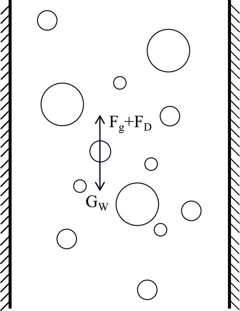
Figure 1. Vertical droplet force analysis diagram.

Turner et al. (1969) established a model based on droplet motion (i.e., the droplet model) by analyzing various forces on the droplet moving along the pipe. According to the characteristics of droplet movement in the pipeline, Turner derived the critical liquid loading model, which is suitable for gas wells. Coleman et al. (2019) found that a certain correlation existed between the average droplet diameters of different liquids. A general relationship was proposed that relates the average droplet diameter to known physical parameters. The droplet diameter was estimated by measuring parameters such as liquid density and surface tension. Droplet deformation occurs when the liquid is carried by high-speed gas (Min et al., 2001). Droplets become ellipsoid during migration, and the modified coefficient in the Turner model changed to 0.38. Four droplets models are mainly listed and compared (Table 1).

Table 1

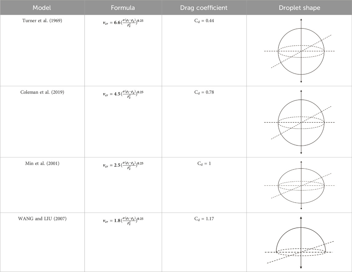
Table 1. Comparison of liquid loading models in the vertical section.

2.2 Calculation model of critical liquid loading output in the inclined section

The principle of liquid loading in the inclined section of horizontal wells is more complicated than that in the vertical section due to the deformation of the droplet when coming into contact with the lower part of the pipe wall under the action of gravity, thus generating frictional resistance. This problem can be solved by analyzing the force of a single droplet in the inclined tube.

The droplet is commonly regarded as a hemispherical body. The effects of gravity, surface tension, and viscous resistance on its force should be considered. When the inclination angle is small, the droplet will roll along the lower part of the tube wall. The droplet will escape from the tube wall when the inclination angle reaches a certain degree, and the friction resistance between the droplets and the tube wall has a significant effect. When the droplet slides on the surface of the tube wall, wetting hysteresis and droplet deformation occur. The droplet forms the advancing contact angle and the receding contact angle [Figure 2 (Wenying LI., 2015)].

Figure 2

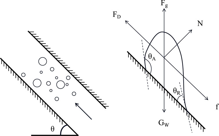
Figure 2. Diagram of droplet force analysis in the inclined tube (Wenying LI., 2015).

In the inclined section, the force is more complicated than that in the vertical section due to the normal force and friction of the wall. The droplet model was improved by adding an angle variable to consider the influence of the angle of inclination on the critical liquid loading. A critical liquid loading model suitable for highly inclined wells and horizontal wells was established by Fiedler shape function, which reflects the relationship between the critical liquid loading velocity and inclination angle (Qian et al., 2022).

The influence of the angle of inclination on critical liquid loading is discussed by Belfroid et al. (2008). The model is expressed as follows Eq. (1):

${\mathit{v}}_{\mathit{c}\mathit{r}}=\mathbf{4.45}{\left(\frac{\mathit{\sigma }\left({\mathit{\rho }}_{\mathit{l}}-{\mathit{\rho }}_{\mathit{g}}\right)}{{\mathit{\rho }}_{\mathit{g}}^{\mathbf{2}}}\right)}^{\mathbf{0.25}}\frac{{\left(\mathit{sin}\left(\mathbf{0.7}\mathit{\theta }\right)\right)}^{\mathbf{0.38}}}{\mathbf{0.74}},(1)$

where $v_{cr}$ is the critical liquid loading rate, $\sigma$ is the surface tension, ${\rho }_l$ is the density of the liquid, ${\rho }_g$ is the density of the gas, and $\theta$ is the angle of inclination.

Angle variables were added to the droplet model, and a series of experiments were conducted. The angle of inclination significantly affects the occurrence of critical liquid loading [Figure 3 (Xianting, 2019)]. The critical liquid loading capacity is weakened due to the uneven distribution of the liquid when the angle of inclination increases. The model has important implications for the understanding of liquid motion and transport properties. A critical liquid loading model suitable for highly deviated wells and horizontal wells is established.

Figure 3

Figure 3. Inclined tube droplet model (Xianting, 2019).

Li et al. (2012) established a new model based on Newton’s law of friction to improve the accuracy of model predictions during liquid dripping. A new numerical method was proposed to model the drip process by considering the friction and adhesion between the droplet surface and the environment. It was simulated using high-performance computing techniques. The model describes the motion, deformation, and splitting process of the droplet more accurately. It should be noted that the Turner model is one of the classical models of the droplet formation and splitting process since it is based on the physical principles of mass conservation, momentum conservation, and energy conservation. Therefore, the model based on Newton’s law of friction was established Eq. (2):

${\mathit{v}}_{\mathit{c}\mathit{r}}=\mathbf{5.5}{\left(\mathit{\lambda }\mathit{sin}\mathit{\theta }+\mathit{cos}\mathit{\theta }\right)}^{\mathbf{0.25}}{\left(\frac{\mathit{\sigma }\left({\mathit{\rho }}_{\mathit{l}}-{\mathit{\rho }}_{\mathit{g}}\right)}{{\mathit{\rho }}_{\mathit{g}}^{\mathbf{2}}}\right)}^{\mathbf{0.25}},(2)$

where $v_{cr}$ is the critical liquid loading rate, $\sigma$ is the surface tension, ${\rho }_l$ is the density of the liquid, ${\rho }_g$ is the density of the gas, $\lambda$ is the friction coefficient, and $\theta$ is the angle of inclination.

However, the model does not consider the interaction between droplets, which is too ideal. Guan et al. (2011) introduced a new model Eq. (3) for angle change by using a similar method:

${\mathit{v}}_{\mathit{c}\mathit{r}}=\mathbf{4.442}{\left(\frac{\mathit{R}\mathit{e}\mathit{cos}\mathit{\theta }}{{\mathit{C}}_{\mathit{D}}\mathit{R}\mathit{e}-\mathbf{16}}\right)}^{\mathbf{0.25}}{\left(\frac{\mathit{\sigma }\left({\mathit{\rho }}_{\mathit{l}}-{\mathit{\rho }}_{\mathit{g}}\right)}{{\mathit{\rho }}_{\mathit{g}}^{\mathbf{2}}}\right)}^{\mathbf{0.25}},(3)$

where $v_{cr}$ is the critical liquid loading rate, $\sigma$ is the surface tension, ${\rho }_l$ is the density of the liquid, ${\rho }_g$ is the density of the gas, $Re$ is the Reynolds number, $C_D$ is the drag coefficient, and $\theta$ is the angle of inclination.

The traditional model for calculating critical liquid loading production had a problem of modified coefficients for the gas wells with a gas–liquid ratio greater than 1,400 m³/m³. YANG et al. (2009) proposed a new calculation model to predict the critical liquid loading gas rate by considering the change in the droplet shape in the wellbore and the relationship between the drag coefficient and Reynolds number. It was assumed that the droplet in the gas wellbore was flat, and classical mechanics was used to create a new model Eq. (4):

${\mathit{v}}_{\mathit{c}\mathit{r}}=\mathbf{3}{\left(\frac{\mathit{\sigma }\left({\mathit{\rho }}_{\mathit{l}}-{\mathit{\rho }}_{\mathit{g}}\right)}{{\mathit{\rho }}_{\mathit{g}}^{\mathbf{2}}}\right)}^{\mathbf{0.25}},(4)$

where $v_{cr}$ is the critical liquid loading rate, $\sigma$ is the surface tension, ${\rho }_l$ is the density of the liquid, and ${\rho }_g$ is the density of the gas.

Chen et al. (2016) proposed a new liquid film model considering the influence of the pipe wall on the liquid droplet (Figure 4). Compared with the Belfroid model, it better matches experimental data. On the basis of the Turner model form, the modified coefficient K_u is added to obtain a new model Eq. (5):

${\mathit{v}}_{\mathit{c}\mathit{r}}=\frac{{\mathit{K}}_{\mathit{u}}}{\mathbf{3.73}}\left(\mathbf{6.6}{\left(\frac{\mathit{\sigma }\left({\mathit{\rho }}_{\mathit{l}}-{\mathit{\rho }}_{\mathit{g}}\right)}{{\mathit{\rho }}_{\mathit{g}}^{\mathbf{2}}}\right)}^{\mathbf{0.25}}\right),(5)$

where $v_{cr}$ is the critical liquid loading rate, $\sigma$ is the surface tension, ${\rho }_l$ is the density of the liquid, ${\rho }_g$ is the density of the gas, $K_u$ is the modified coefficient, and $\theta$ is the angle of inclination.

Figure 4

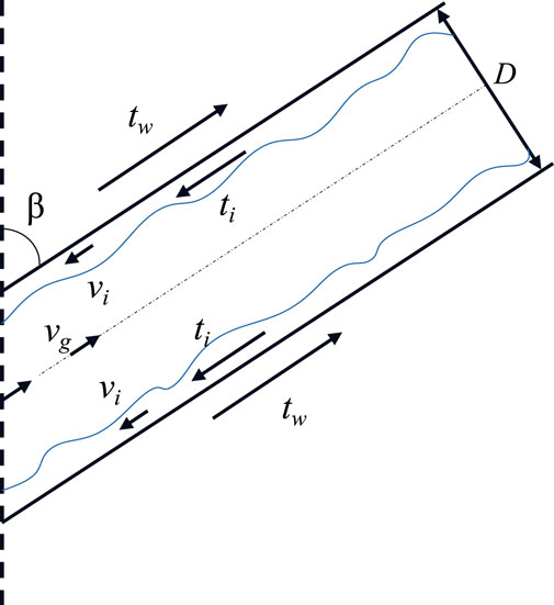
Figure 4. Schematic diagram of the liquid film flow model (Chen et al., 2016).

2.3 Calculation model of critical liquid loading output in the horizontal section

When the gas–water phase flows in the horizontal section, whether the liquid in the horizontal section can be completely carried into the inclined section depends on whether the flow pattern changes in the horizontal section (Wenying Li, 2015). It is necessary to form an annular mist flow to completely carry the liquid in the horizontal section into the inclined section when there is a stratified flow of gas and water.

2.3.1 Stratified flow model

When the velocity of the liquid and gas is different, the interface between them will fluctuate. These fluctuations increase unsteadily, the morphology of the gas–liquid interface changes eventually, and the flow pattern changes from a stratified flow to annular mist flow. The gas phase velocity and liquid level height are important to this transformation. The fluctuations at the interface are more easily amplified under the high speed of gas or a low liquid level, so the stratified flow transforms into a ring mist flow. On the contrary, the stratified flow is maintained for a longer time.

Taitel and Dukler believed that the gas and liquid phases in the horizontal section usually exhibit a stratified flow pattern when the influence of the radial inflow of horizontal wells is considered (Taitel and Dukler, 1976); the liquid film at the bottom of the pipe becomes thicker than the liquid film at the top, and then, the liquid loads in wells. Xiao and Yingchuan (2010) believed that the horizontal section has no significant effect on the infusion of horizontal wells. Figure 5 (Xiao and Yingchuan, 2010) shows the stratified flow model of a horizontal well.

Figure 5

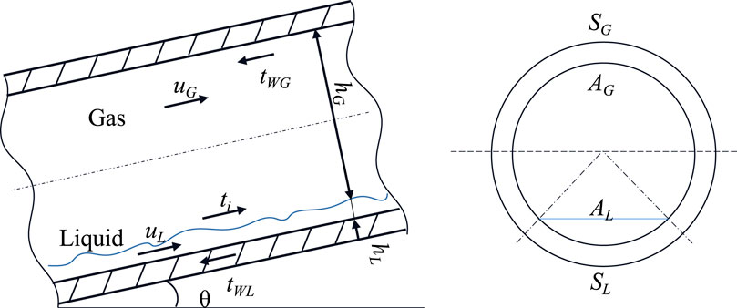
Figure 5. Schematic diagram of the hierarchical flow model (Taitel and Dukler, 1976).

2.3.2 Carrying sedimentation mechanism model

The droplets in the gas–liquid mixture move with the gas instead of just settling at the bottom. This mechanism is also known as the “entrainment effect” since the droplets are entrained by the gas (Pan and Hanratty, 2002). In a horizontal tube, the liquid settles around the wall to form a liquid film. This phenomenon can be described by the horizontal tube layered flow model, as shown in Figure 6 (Pan and Hanratty, 2002).

Figure 6

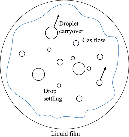
Figure 6. Schematic diagram of the loading settlement mechanism (Pan and Hanratty, 2002).

In the case of a higher gas velocity, part of the liquid flows along the tube wall, while the other part is dispersed into droplets carried in the air flow. Droplet carrying can be considered the result of the balance between the liquid film carrying rate and the droplet settling rate. When the liquid film carrying rate and the droplet carrying rate are equal, the atomization amount of the liquid film is equal to the droplet settling amount, thus forming continuous droplet carrying (Pan and Hanratty, 2002). It can be concluded that the critical liquid loading velocity Eq. (6) is expressed as

${\mathit{v}}_{\mathit{c}\mathit{r}}=\frac{\mathbf{32}{\mathit{\sigma }}^{\mathbf{5}/\mathbf{14}}}{{\mathit{\rho }}_{\mathit{g}}^{\mathbf{5}/\mathbf{14}}{\mathit{D}}^{\mathbf{3}/\mathbf{14}}},(6)$

where $v_{cr}$ is the critical liquid loading rate, $\sigma$ is the surface tension, ${\rho }_g$ is the density of the gas, and $D$ is the pipe diameter.

2.3.3 Kelvin–Helmholtz instability theory model

The Kelvin–Helmholtz instability theory model is used to describe the change in the gas–liquid interface waveform. Based on the principle of fluid dynamics and stability analysis, small-scale vortices become unstable due to the different velocities and friction of two fluids under a high rate of gas flow, thus causing interface fluctuations (ZHAO, 2019). As the gas velocity increases gradually, the liquid film moves along the tube wall and drives the formation of liquid droplets due to the interface instability fluctuation.

Andritsos and Hanratty (1987) found that the instability of Kelvin–Helmholtz fluctuations led to the generation of large irregular fluctuations. When the gas velocity became twice the critical value, the interfacial fluctuations led to the distribution of the liquid film around the tube wall and the formation of liquid droplets. The calculation model of the critical gas velocity of continuous liquid loading in horizontal tubes is expressed Eq. (7) as follows:

${\mathit{v}}_{\mathit{c}\mathit{r}}=\mathbf{2}\sqrt{\mathbf{2}}{\left(\frac{\mathit{g}\mathit{\sigma }{\mathit{\rho }}_{\mathit{l}}}{{\mathit{\rho }}_{\mathit{g}}^{\mathbf{2}}}\right)}^{\mathbf{0.25}},(7)$

where $v_{cr}$ is the critical liquid loading rate, $\sigma$ is the surface tension, ${\rho }_l$ is the density of liquid, ${\rho }_g$ is the density of gas, and $g$ is the gravitational acceleration.

3 Field cases of critical liquid loading models

3.1 Application in the ZJ gas field

The ZJ gas field is located in the transitional zone between the eastern slope of the western Sichuan hollow and the central Sichuan uplift in the Sichuan Basin, China. It is an ultra-low permeability and low-porosity tight sandstone gas reservoir. Since its development in 2012, more than 200 gas wells have been put into production. The bottomhole back pressure increases continuously due to the loading of formation water, and the gas well output decreases rapidly; thus, the stable production time of most individual wells is less than 2 years. The wellhead pressure of the gas well in the ZJ gas field mainly ranges from 2 to 20 MPa. The average coefficient of compressibility is 0.85, the temperature is 323 K, the water density is 1,074 kg/m³, the relative density of natural gas is 0.6, and the water–gas interfacial tension is 0.06 N.

The Li model, Belfroid model, and Kelvin–Helmholtz instability theory model (Andritsos and Hanratty, 1987) were selected as the critical liquid loading models for vertical, inclined, and horizontal sections, respectively, by Yunyang (2021). The liquid loading state is marked on the relationship diagram between critical liquid loading flow and daily gas production. The unloaded area is above the diagonal line, and the loaded area is below the diagonal line.

Figure 7A shows the inaccurate calculated results of the Turner model, and the wells unloaded and wells nearly loaded are obviously inconsistent with the field situation. The results of the Li model coincided with field data (Figure 7B) (Yunyang, 2021), and the effectiveness of application in vertical wells was verified. The results of the Belfroid model and Kelvin–Helmholtz instability theory model also coincided with field data (Figures 7C, D), and the accuracy of prediction met the requirements.

Figure 7

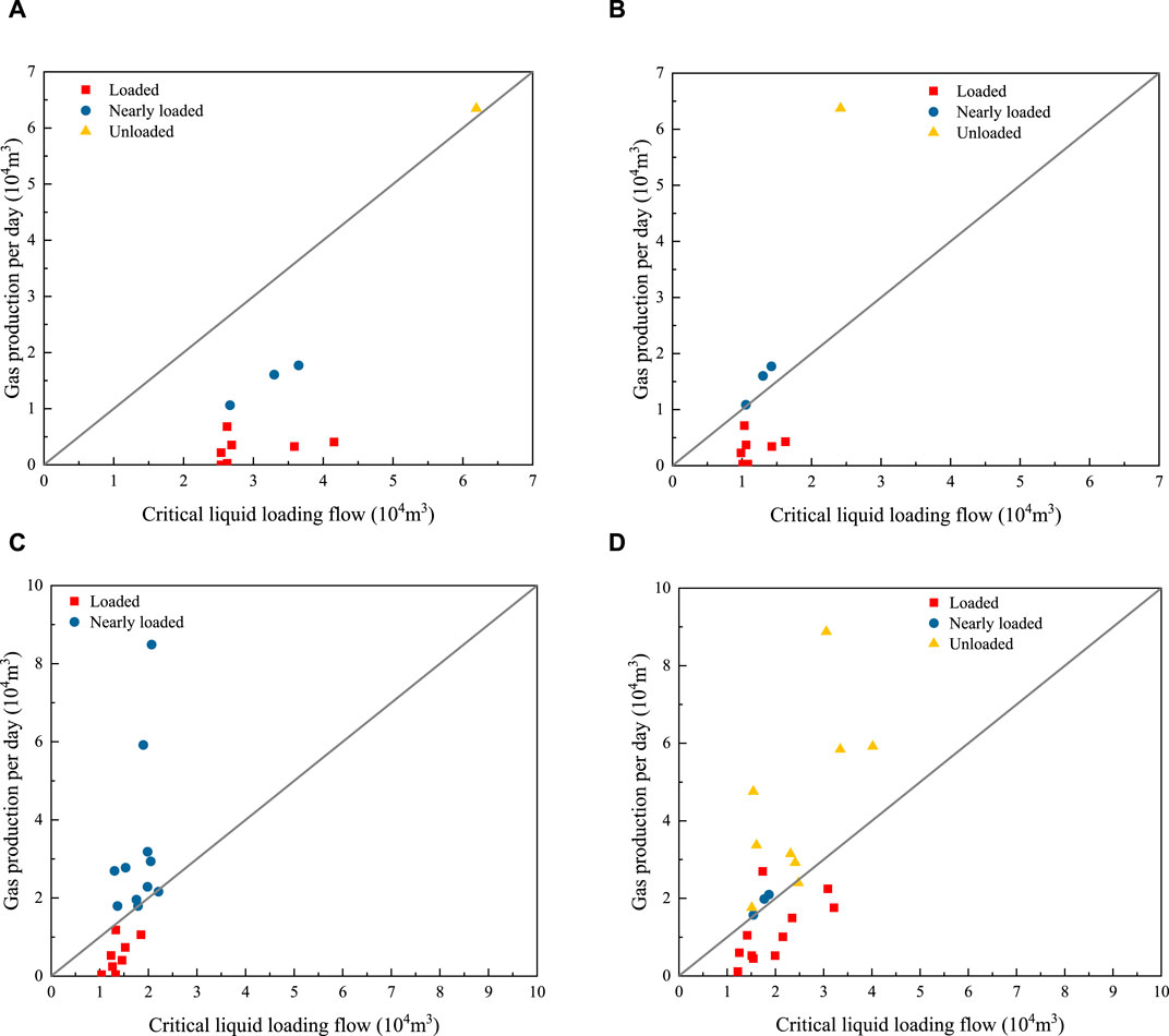
Figure 7. (A) Turner model. (B) Li model. (C) Belfroid model. (D) Kelvin–Helmholtz instability theory model (Yunyang, 2021).

The analysis of 55 low-pressure gas wells in the ZJ gas field shows that the coincidence rate is 93%, which proves that the selected model and the modified model can effectively predict the liquid loading of the gas wells in the ZJ gas field. On the basis of previous research results, established simplified calculation models of the critical liquid carrying flow in the ZJ gas field. As long as the wellhead pressure, tubing inner diameter, and well inclination angle are obtained, the critical liquid carrying flow rate and flow rate can be calculated, which is convenient for field application.

3.2 Application in the FL gas field

Existing geological data and productivity evaluation show that the FL shale gas field has 2.1 trillion m³ of resources, which is the first large-scale shale gas field in China and the largest shale gas field in the world except North America. In order to establish a new model of critical liquid loading production suitable for this gas field, Zhao and Liu (2019) calculated the average droplet diameter by using the equilibrium relationship between the droplet surface free energy and the turbulent kinetic energy of the gas phase. They comprehensively considered the influence of the inclination angle on the continuous liquid loading of the droplets and used the Fiedler function to modify it.

The new model determines the droplet diameter based on the equilibrium relationship between the surface free energy of the droplets and the turbulent kinetic energy of the gas phase. At the same time, the influence of well inclination is considered. The Turner model is modified as follows Eq. (8):

${\mathit{v}}_{\mathit{c}\mathit{r}}=\mathbf{4.667}{\left[\frac{\mathit{\sigma }\left({\mathit{\rho }}_{\mathit{l}}-{\mathit{\rho }}_{\mathit{g}}\right){\mathit{Q}}_{\mathit{s}\mathit{l}}}{{\mathit{D}}^{\mathbf{1.8}}{{\mathit{\mu }}_{\mathit{g}}^{\mathbf{0.2}}\mathit{\rho }}_{\mathit{g}}^{\mathbf{1.8}}}\right]}^{\frac{\mathbf{1}}{\mathbf{4.8}}}\frac{{\mathbf{sin}\left(\mathbf{1.7}\mathit{\theta }\right)}^{\mathbf{0.38}}}{\mathbf{0.74}},(8)$

where $v_{cr}$ is the critical liquid loading rate, $\sigma$ is the surface tension, ${\rho }_l$ is the density of the liquid, ${\rho }_g$ is the density of the gas, $Q_{sl}$ is the liquid flow, $D$ is the pipe diameter, and $\theta$ is the angle of inclination.

Zhao and Liu used 10 different models, including those proposed by Turner et al. (1969), Coleman et al. (2019), Li et al. (2012), Belfroid, and the model modified by Zhao and Liu, to predict the wellbore liquid loading of three kinds of pipe diameters (2–3/8′, 2–7/8′, and 5–1/2′) in the FL shale gas field. By comparing the field liquid loading of gas wells, the accuracy of various critical liquid loading models for judging the liquid loading in gas wells with different pipe diameters was analyzed (Figure 8) (Zhao and Liu, 2019). The model modified by Zhao and Liu has the highest discrimination accuracy and the most accurate prediction, with an average accuracy of 90%.

Figure 8

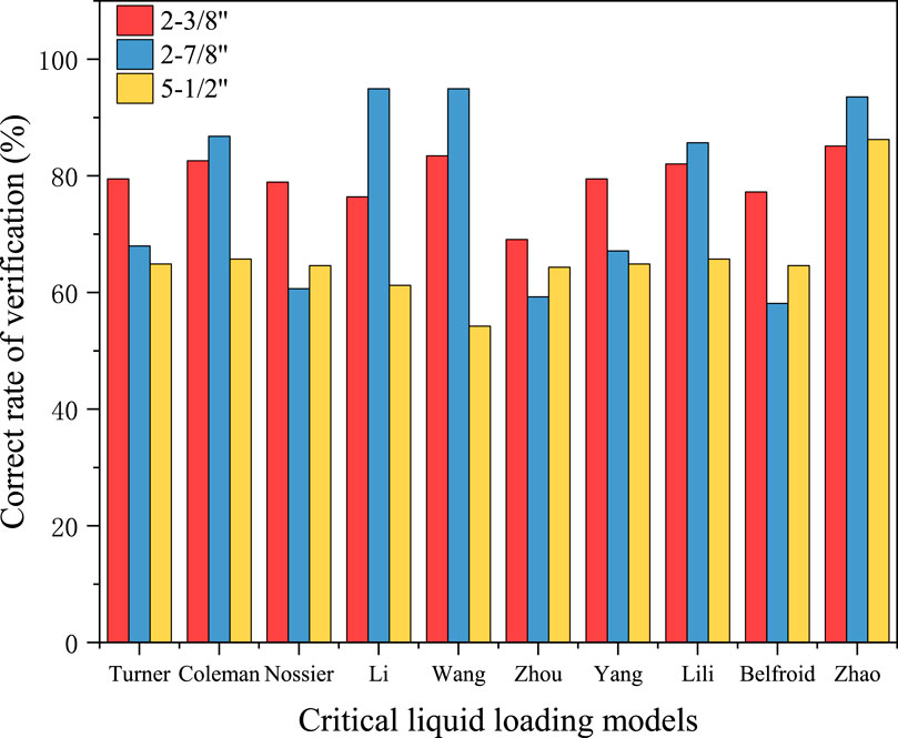
Figure 8. Comparison of critical liquid loading models (Zhao and Liu, 2019).

Compared with the field flow rate of the gas well, the loading position of the well in different production periods was judged and analyzed. Well X1 of the FL gas field was taken as an example.

3.2.1 Casing production period

Data from the casing production period of the well were substituted into the new critical liquid loading model established to analyze the liquid loading situation of the well. The critical liquid loading flow curve is shown in Figure 9 (Zhao and Liu, 2019).

Figure 9

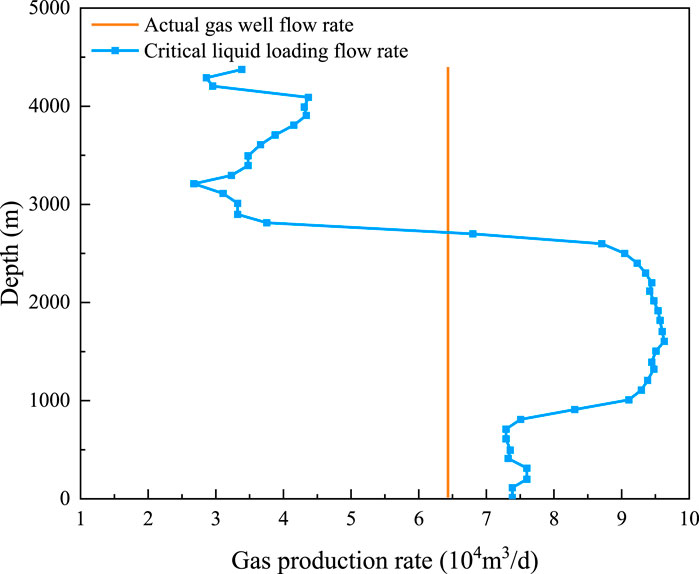
Figure 9. Critical loading flow rate curve (casing) (Zhao and Liu, 2019).

The critical liquid loading flow rate at each shallow position of the 2,600-m shaft of well X1 is greater than the field flow rate of the gas well (Figure 9); it is difficult for the gas well to load the liquid. Below the depth of 2,600 m, the critical liquid loading flow rate of each position is less than the field flow rate of the gas well, and the gas well shaft can load the liquid normally.

3.2.2 Tubing production period

Compared to the liquid loading curve observed during casing production, the critical liquid loading flow rate of the wellbore during tubing production experiences a significant decrease. This reduction can be attributed to the decrease in the inner diameter of the production string after the tubing is run, and the liquid loading capacity for the gas well is enhanced (Figure 10) (Zhao and Liu, 2019). The gas well enters the casing production section, the liquid loading capacity weakens, and the critical liquid loading flow rate increases. Conversely, as the gas well shaft enters the horizontal section, the liquid loading capacity increases, while the critical liquid loading flow decreases.

Figure 10

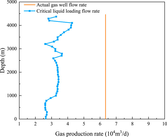
Figure 10. Critical loading flow rate curve (tubing) (Zhao and Liu, 2019).

The critical liquid loading flow at each position of well X1 is lower than the field flow of the gas well, indicating that the gas well is able to carry the liquid normally. The model established by Zhao and Liu is superior to the traditional model and has better accuracy.

3.3 Application in the DND gas field

The accumulated proved reserves of the DND gas field are 416.83 billion m³, the used reserves are 190.55 billion m³, and the reserve utilization rate is only 45.71%. The quality of the remaining unused reserves is poor, so it is difficult to realize economic and effective development through conventional vertical well mining.

Based on the basic data on 230 vertical wells in the DND gas field, ZHOU et al. (2013) proposed a model of critical liquid loading in the vertical section of the DND gas field on the basis of the Turner model Eq. (9):

${\mathit{v}}_{\mathit{c}\mathit{r}}=\mathbf{2.35}{\left[\frac{\mathit{\sigma }\left({\mathit{\rho }}_{\mathit{l}}-{\mathit{\rho }}_{\mathit{g}}\right)}{{\mathit{\rho }}_{\mathit{g}}^{\mathbf{2}}}\right]}^{\mathbf{0.25}},(9)$

where $v_{cr}$ is the critical liquid loading rate, $\sigma$ is the surface tension, ${\rho }_l$ is the density of liquid, and ${\rho }_g$ is the density of gas.

The model modified by ZHOU et al. (2013) was used to predict the liquid loading states of 230 vertical wells. Among these wells, 28 wells were misjudged, with an accuracy rate of 87.7%. It was sufficient to meet the field production needs of the DND gas field (Figure 11).

Figure 11

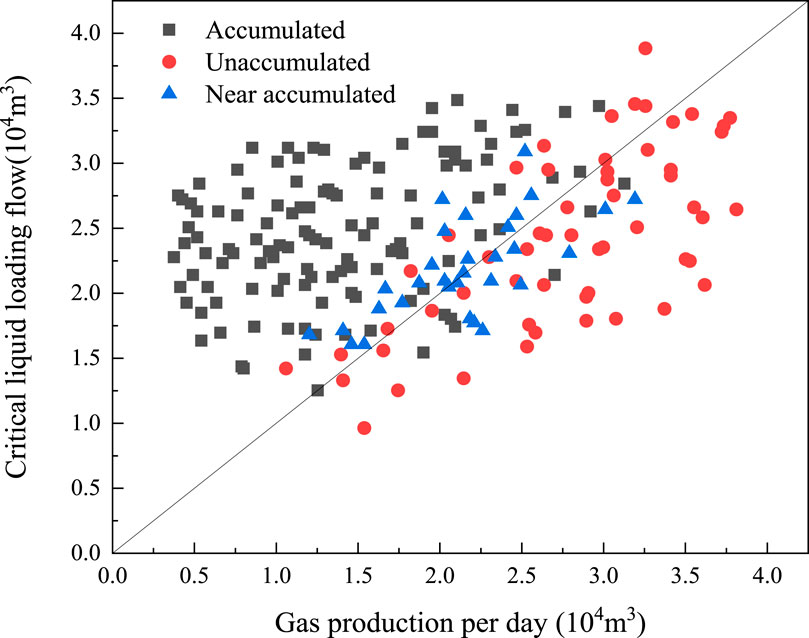
Figure 11. Calculation results of the critical liquid loading model in the vertical section (ZHOU et al., 2013).

The stratified flow model, the loading settlement mechanism model, and the Kelvin–Helmholtz instability theory model were mainly used to establish the simulation experiment for the horizontal section. The continuous liquid loading simulation experiment device in the horizontal section was prepared, as shown in Figure 12 (ZHOU et al., 2013).

Figure 12

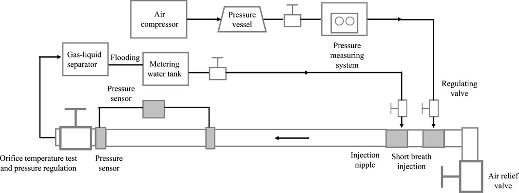
Figure 12. Continuous liquid loading simulation experimental device in the horizontal well section (ZHOU et al., 2013).

The changes in gas flow on the formation, distribution, and loading of liquid droplets were observed under a certain liquid flow rate. The form of the liquid film in the horizontal pipe and the changes in the two-phase gas–liquid flow pattern were recorded. The pressure, temperature, injected gas volume, and injected pressure in the test pipe section were tested to accurately simulate continuous liquid loading in horizontal wells.

The experimental data under different wellhead pressures were compared with the calculated values of three horizontal section theoretical models (Figure 13) (ZHOU et al., 2013). The calculated value of the carrying sedimentation mechanism model is too high, and the value of the stratified flow model is too low. The calculated value of the Kelvin–Helmholtz fluctuation theory model is the most accurate. The liquid loading in the horizontal pipe is mainly caused by the fluctuations at the gas–liquid interface, which is consistent with the liquid loading phenomenon in the horizontal pipe observed in the experiment.

Figure 13

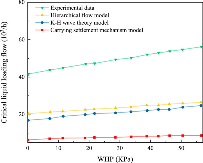
Figure 13. Comparison between the field data and the calculated values of the model (ZHOU et al., 2013).

For the inclined section, ZHOU et al. (2013) designed a continuous liquid loading simulation experiment in a highly inclined well (Figure 14) and carried out a critical liquid loading experiment in an inclined well with inclination angles of 20°, 40°, and 60°. The critical gas volume under different water volumes, gas volumes, pressures, and temperatures was tested by changing the injected water volume and gas volume. The above steps were repeated by changing the angle of inclinations. Finally, the critical gas volume under different inclination angles and different liquid flow velocities was obtained (ZHOU et al., 2013).

Figure 14

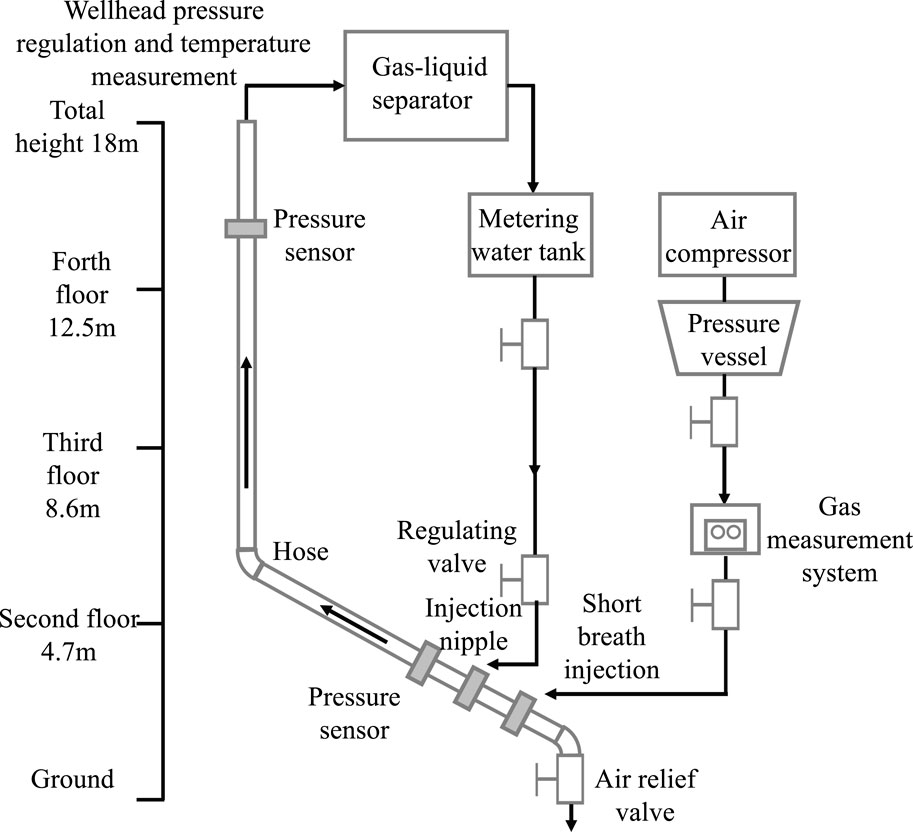
Figure 14. Simulation device experiment flowchart (ZHOU et al., 2013).

A modified model of the inclined tube was obtained by fitting the critical liquid loading capacity under different inclination angles Eq. (10):

${\mathit{v}}_{\mathit{c}\mathit{r}}=\mathbf{4.3}{\left(\frac{\mathit{\sigma }\left({\mathit{\rho }}_{\mathit{l}}-{\mathit{\rho }}_{\mathit{g}}\right)}{{\mathit{\rho }}_{\mathit{g}}^{\mathbf{2}}}\right)}^{\mathbf{0.25}}\frac{{\left(\mathbf{sin}\left(\mathbf{1.7}\mathit{\theta }\right)\right)}^{\mathbf{0.38}}}{\mathbf{0.74}},(10)$

where $v_{cr}$ is the critical liquid loading rate, $\sigma$ is the surface tension, ${\rho }_l$ is the density of the liquid, ${\rho }_g$ is the density of the gas, and $\theta$ is the angle of inclination.

The inclined tube droplet model, liquid film model, and modified model were adopted. The test data were calculated, and the error statistics are shown (Table 2).

Table 2

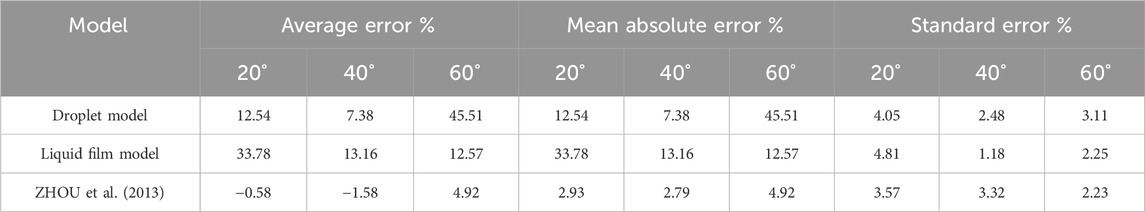
Table 2. Statistical table of errors of the liquid loading model in the inclined pipe (ZHOU et al., 2013).

The model modified by ZHOU et al. (2013) has the smallest error, and its calculation results are superior to those of the droplet model and liquid film model. The model can be used as the calculation model for the critical liquid loading capacity of the inclined pipe.

According to the field situation of the DND gas field, ZHOU et al. (2013) designed the continuous liquid load simulation experiment of the horizontal well and the continuous liquid load simulation experiment of the high-inclination well. Based on the classical critical fluid loading model established by predecessors, a reasonable horizontal well continuous fluid loading model was obtained by considering the influence of the inclination angle and horizontal section length. The calculation results of the example show that the accuracy is 94.4%, which meets the engineering requirements.

3.4 Application in the WY block

The WY shale gas field (herein referred to as the WY block) is within the scope of the CN-WY national shale gas demonstration zone. It is a large-dome anticlinal structure belonging to the low steep fold belt of southwest Sichuan in the central uplift area of the Sichuan Basin (WANG et al., 2012). Yunsheng et al. (2019) studied the geological and engineering parameters and production rules of six horizontal wells of the PT2 platform and put forward development suggestions.

The construction area of the WY block is one wing of an anticlinal structure. The drilling direction of the horizontal well is almost perpendicular to the buried depth contour. As a result, there are generally cases of updip in the upper-half branch and downdip in the lower-half branch (WANG et al., 2016). By comparing the current gas well production with the critical liquid loading rate, it is concluded that 63 of the 89 platform wells were loaded in varying degrees. Most of these wells are located in the upper half of the block (WANG et al., 2014a).

Due to the difference in the drilling location and engineering parameters, the production and pressure changes between the upper- and lower-half branches of the development platform in the WY block are quite different (WANG et al., 2014b). Meanwhile, due to the large amount of fracturing fluid in the ground, gas wells produce liquid for a long period of time in the early stage of operation (WANG et al., 2009). Flowback fluid will have a great impact on the output of gas wells (LIAO et al., 2009).

Fractures of shale gas wells produce a significant amount of liquid along with the gas at the initial stage. The problem of liquid loading becomes crucial by using casing for production. The Li model (Min et al., 2002) was chosen to determine the critical liquid loading flow rate when using the wellhead as the reference point. The relative density of the gas produced by horizontal wells on the PT2 platform was 0.5684, and the water density was 1,030 kg/m³. The inner diameter of the casing was 114.3 mm, the average wellhead temperature was recorded at 310 K, and the gas–water interfacial tension was 0.06 N/m. The critical liquid loading flow rate for various casing pressures were calculated by applying the Li model. The casing pressure and gas production data on six horizontal wells on the PT2 platform are shown in Figure 15 (Yunsheng et al., 2019).

Figure 15

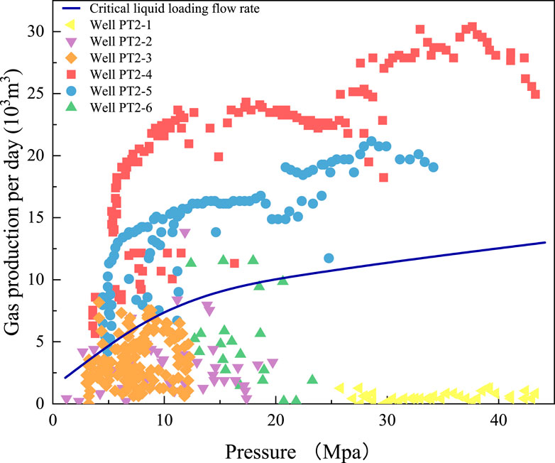
Figure 15. Comparison of gas production and the critical liquid loading flow of six wells in the PT2 platform under different casing pressures (Yunsheng et al., 2019).

The gas production of shale gas wells is affected not by the quality of the drilled reservoir, the effect of fracturing reconstruction, and the flowback fracturing fluid in the formation. If the gas production of the well is lower than the critical liquid loading flow, the liquid will accumulate at the bottom of the well. The gas productions per day of well PT2-4 and well PT2-5 were higher than the critical liquid loading flow rate, and the liquid was carried out from the bottomhole continuously by the gas flow. The gas productions per day of well PT2-1, well PT2-2, well PT2-3, and well PT2-6 were lower than the critical liquid loading flow rate, and liquid was loaded. For low-producing wells, it is recommended to use small tubing (tubing bore diameter less than or equal to 62 mm). For the upper half of low-producing wells, skid-mounted drainage gas production tools and measures should be taken early to release gas well productivity, and for the lower half of low-producing wells, pressure production should be released to prevent premature liquid loading at the bottom of the well.

3.5 Application in the CN shale gas area

Two kinds of horizontal wells exist for shale gas in the CN area: upwarped horizontal wells and downdip horizontal wells. A visual simulator for two-phase gas–liquid wellbore pipe flow was built by Liu (2019), which was designed by Na et al. (2007). A critical liquid gas loading velocity mathematical model suitable for the CN shale gas horizontal well was established.

3.5.1 Experimental process

In order to observe the law of two-phase flow in the horizontal section of the CN shale gas horizontal gas well directly, a physical simulation experimental device for the drainage and production of horizontal gas wells was designed and built according to the field production parameters of horizontal gas wells (Figure 16). The experimental device consists of a gas supply system, liquid system, experimental flow pipeline system, test system, and data monitoring system. The total size of the experiment is 6.5 m, and the inner diameter of the experiment pipeline is 30 mm (three kinds of pipe diameters: 30, 40, and 50 mm). A pressure gauge was set in the horizontal section of the experiment pipe section, a pressure regulator was set in the vertical section 3.5 m high (the measurement result is the wellhead pressure), and a pressure gauge was set in the horizontal section (the measurement result is the bottom-hole pressure). A horizontal section length of 6.0 m was built to be replaced with three kinds of pipe diameters. It was equipped with the corresponding supply equipment and monitoring system, which can be used to simulate the drainage and gas production process of horizontal wells under different pipe diameters.

Figure 16

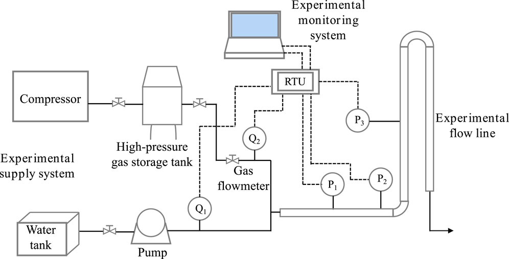
Figure 16. Experimental flowchart (Liu, 2019).

The air was compressed and stored in the gas storage tank as a supply system; then, it was transported to the intake pipeline and then to the experimental pipeline to join the liquid. The tap water provided by the faucet flows out to the water tank and enters the water pipeline through the pump. The gas and liquid are mixed in the pipeline and entered the experimental pipeline. A high-definition digital camera was used to record the flow pattern changes in the flow pipeline. A pressure sensor, gas flowmeter, and liquid flowmeter were used to display the bottomhole pressure, wellhead pressure, intake gas, intake liquid, and other parameters; the experimental test data were recorded using the data monitoring system in real time. During the experiment, the formation, loading, and settling of droplets, the adjustment of gas injection, and the distribution and movement of the liquid film in the tube section were observed. When the flow rate of this section reached the stable critical liquid loading state, the data on gas injection, water injection, wellhead pressure, and wellhead temperature were recorded. After one set of tests, the pressure value of the test section was changed by the pressure regulator, and the next set of tests was carried out. The critical flow data on liquid loading under different wellhead conditions were obtained by repeating the appeal operation.

3.5.2 Analysis of experimental results

For the upwarped horizontal well model, the angle between the horizontal section and the horizontal direction was 5°. Based on the Kelvin–Helmholtz instability theory model, experiments were carried out under clean water with pipe diameters of 30 mm, 40 mm, and 50 mm. A series of modified coefficients were obtained. The average modified coefficient was 4.363. The critical liquid loading model of upwarped horizontal wells Eq. (11) is represented as follows:

${\mathit{v}}_{\mathit{c}\mathit{r}}=\mathbf{4.363}{\left(\frac{\mathit{g}\mathit{\sigma }{\mathit{\rho }}_{\mathit{l}}}{{\mathit{\rho }}_{\mathit{g}}^{\mathbf{2}}}\right)}^{\mathbf{0.25}},(11)$

where $v_{cr}$ is the critical liquid loading rate, $\sigma$ is the surface tension, ${\rho }_l$ is the density of the liquid, ${\rho }_g$ is the density of the gas, and $g$ is the gravitational acceleration.

Under the same pipe diameter condition, the critical liquid loading model of the downdip horizontal well Eq. (12) is obtained:

${\mathit{v}}_{\mathit{c}\mathit{r}}=\mathbf{4.226}{\left(\frac{\mathit{g}\mathit{\sigma }{\mathit{\rho }}_{\mathit{l}}}{{\mathit{\rho }}_{\mathit{g}}^{\mathbf{2}}}\right)}^{\mathbf{0.25}},(12)$

where $v_{cr}$ is the critical liquid loading rate, $\sigma$ is the surface tension, ${\rho }_l$ is the density of the liquid, ${\rho }_g$ is the density of the gas, and $g$ is the gravitational acceleration.

3.5.3 Example calculation

According to the modified models of the critical liquid loading flow of the horizontal well with two kinds of well trajectory obtained in the previous two experiments, the calculation and analysis of the two well types of the CN shale gas horizontal well were carried out. Tables 3, 4 show the analysis and comparison between the critical liquid loading flow value calculated by the models and the field production to diagnose the liquid loading in gas wells.

Table 3

Table 3. Comparison of calculation results of the critical liquid loading capacity in downdip horizontal wells (Liu, 2019).

Table 4

Table 4. Comparison of calculation results of the critical liquid loading capacity in updip horizontal wells (Liu, 2019).

The results obtained by using the modified critical liquid loading model through the simulation experiment exactly coincided with the results obtained by using the echo meter to diagnose the liquid surface. The verification of the field example shows that the horizontal well critical liquid loading flow model modified by Liu can better predict whether there is liquid loading at the bottom of the well in the CN area.

4 Recent new models and validation

4.1 Shekhar model

4.1.1 Theoretical modeling

The model established by Turner et al. (1969) was modified by Belfroid et al. (2008). However, the methods were based on incorrect physical assumptions and did not consider the pipe diameter (Shekhar et al., 2017). Another approach suggested by Shu et al. (2014) employed accurate physical assumptions for liquid loading but was overly cautious. Barnea (1987) proposed a new method that tackles various limitations to previous models. The method modified by Shekhar assumes that when liquid loading begins, the liquid film starts to descend backward. It considers the inclination angle and diameter. The method can predict the position of liquid loading from vertical wells to horizontal wells. The validity of this method is confirmed through comparisons with laboratory and field data.

Liquid load prediction in near-horizontal or inclined wells is different from and more difficult than that in vertical wells. Since the inclination of a typical well ranges from purely vertical to near horizontal, the correlation for predicting liquid loading is flexible enough to predict the position of liquid loading.

Based on experimental observations (Van’t Westende et al., 2007) and the recent literature (Alamu, 2012), it can be inferred that liquid loading occurs when the liquid film begins to fall backward. Alamu (2012) stated that the percentage of liquid in the form of droplets in a gas core is negligible at low gas velocities. Van’t Westende et al. (2007) reported that the droplet size used by Turner et al. (1969) to estimate the critical surface gas velocity is not observed in practice. The Weber number of droplets in the annular flow is less than 30, whereas Turner et al. (1969) used a Weber number of 60 after the same adjustment. Both observations provide additional support for the idea that the most likely cause of liquid loading is liquid film inversion.

Figure 17 (Shekhar et al., 2017) shows the variation in film thickness in vertical and inclined wells. The thickness of the liquid film varies from top to bottom. The thickness of the film is smaller at the top (under gravity) and larger at the bottom. As the angle changes from vertical to near horizontal, the membrane at the bottom of the pipe thickens. The thickness inside the pipe is the same at any circumference. Therefore, the circumference of the pipe can be approximately rectangular. The film thickness changes linearly with the change in the circumferential position of the pipeline (Figure 18) (Shekhar et al., 2017). It can be expanded into a trapezoid, with a maximum film thickness at 180° and a minimum film thickness at 0°.

Figure 17

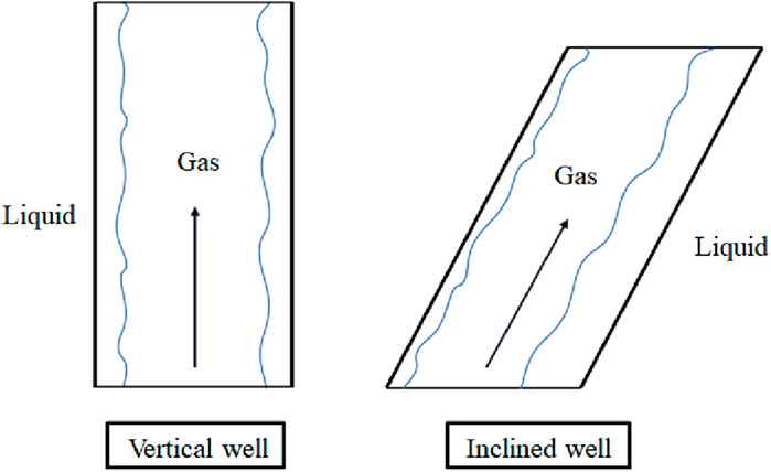
Figure 17. Film thickness in vertical and inclined wells (Shekhar et al., 2017).

Figure 18

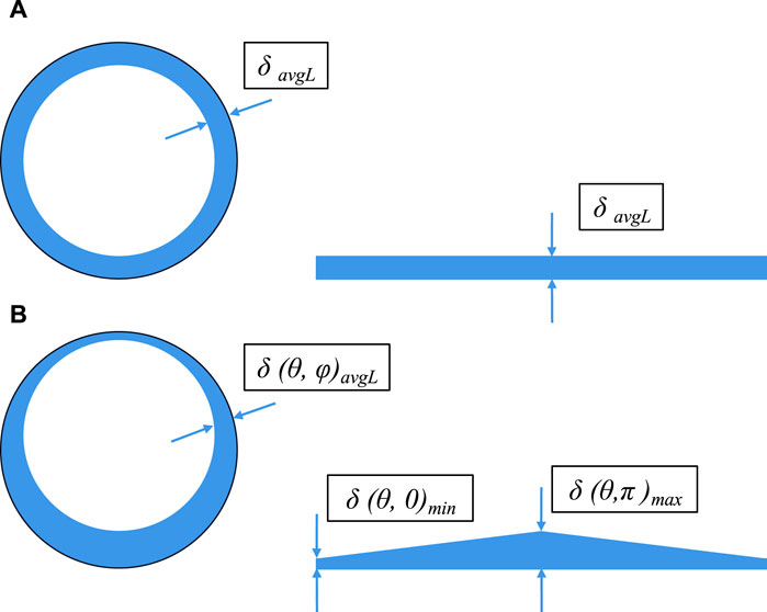
Figure 18. Cross-sectional view of vertical wells (A) and inclined wells (B) (Shekhar et al., 2017).

At the onset of liquid loading, the well experiences annular flow with a fluid film of critical thickness. As the velocity of the gas phase decreases and the film thickness increases, the gas phase faces increasing difficulty in transporting the liquid due to interfacial friction. Consequently, the film starts to recede, and liquid loading commences. The criteria used to determine the critical film thickness are based on the research by Barnea (1986). It is assumed that liquid loading will begin when the thicker film cannot be carried by the gas phase in inclined pipes.

The results obtained by Belfroid et al. (2008) and Shu et al. (2014) were compared with results of the modified model. Predictions of the modified model were more accurate (Figure 19) (Shekhar et al., 2017). Vertical wells have a v_{sg, critical} value of 15.5 m/s. As the inclination angle increases from 0° to 40°, the critical gas velocity increases to 26 m/s. The maximum value is reached at 35°. Beyond 45°, the v_{sg, critical} value decreases until it reaches the minimum of v_sg = 7.3 m/s for a near-horizontal well (88°). It was observed that the v_{sg, critical} values predicted by Shu et al. (2014) were higher and conservative.

Figure 19

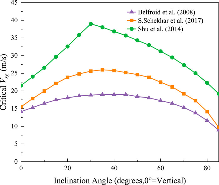
Figure 19. v_{sg, critical} vs. the whole-well inclination range (0°–85°) (Shekhar et al., 2017).

4.1.2 Model verification

To confirm the ability of the method to predict the inception of liquid loading, the results of the proposed method were compared with both laboratory and field data (Tables 5, 6) (Shekhar et al., 2017).

Table 5

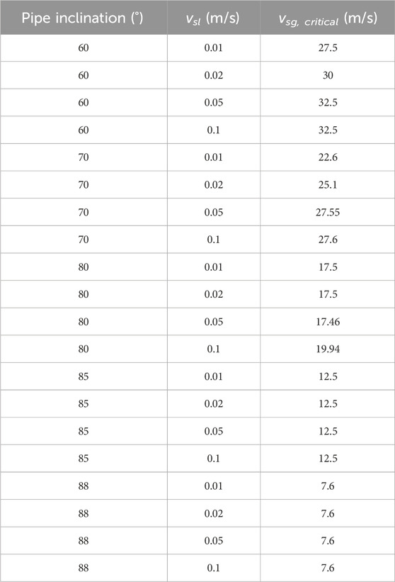
Table 5. Data on the 3-in. pipe liquid loading experiment (Alsaadi, 2013).

Table 6

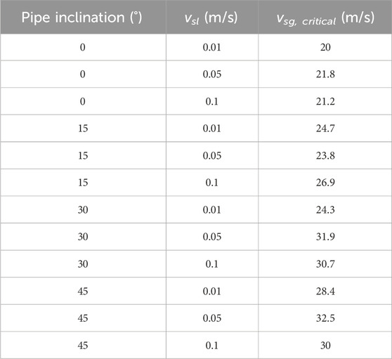
Table 6. Data on the 3-in. pipe liquid loading experiment (Guner, 2012).

4.1.2.1 Experimental verification

The transition boundary is calculated and plotted by using new methods and data from the liquid loading experiments conducted by Guner (2012) and Alsaadi (2013). Starting with the vertical pipe, the data on the pipe inclined at 88° are plotted. The prediction maps obtained by Shu et al. (2014) and Belfroid et al. (2008) were also drawn. Shu et al. (2014) provided consistent conservative results compared to the new approach. In contrast, the modified model was consistent with the experimental data at all angles. The model proposed by Turner et al. (1969) had a constant boundary at v_sg with a critical value of 17 m/s, while that proposed by Belfroid et al. (2008) varied with well inclination. Both are fairly optimistic (lower velocity) predictions for liquid loads relative to laboratory data.

4.1.2.2 Field data verification

Belfroid et al. (2008) shared data from two wells in their paper. One of the wells had a critical gas flow rate of 90,000 standard m³/day, and the other had a critical gas flow rate of 45,000 standard m³/day. The gas-specific gravity of both wells was close to 0.6. These wells had an inclination angle of 40°, and the equations proposed by Belfroid et al. (2008) did not predict the load on these wells (Figure 20). The method suggested by Shekhar et al. (2017) predicted the well load accurately, and the prediction result was close to the 45° line. Figure 20 (Shekhar et al., 2017) plots the critical gas velocity against the observed velocity. The 45° line indicates the start of loading. If the critical velocity is higher than the observed shallow gas velocity, the well will be loaded (i.e., the point will be above the 45° line). If the critical velocity is lower than the field velocity, the well will be in a stable state and unloaded (i.e., the point will be below the 45° line). The predicted value of the critical surface gas velocity should be slightly above or close to the 45° line.

Figure 20

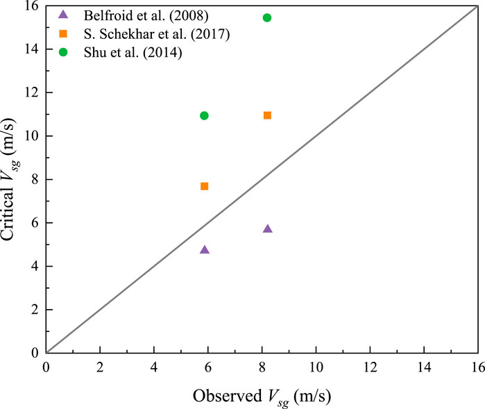
Figure 20. Calculated critical gas velocity vs. measured gas velocity for loading wells studied by Belfroid et al. (2008) (Shekhar et al., 2017).

The dataset proposed by Coleman et al. (1991) has low wellhead pressures, typically less than 500 psia. The mean surface temperature for the dataset is approximately 117°F. All the wells were vertical and began to show fluid loading. The well is on the boundary between unloading and loading conditions. The predicted critical speed should be slightly above the 45° line. The dataset contains information on 56 wells. Compared with other models, the model modified by Shekhar et al. (2017) has a better predictive effect on the liquid loading start time of this dataset. Most of the points on the observed and calculated critical gas velocity curves are located at or close to the 45° line (Figure 21). A comparison with the model of Shu et al. (2014) shows that this model is more conservative than the model modified by Shekhar et al. (2017) (Figure 21).

Figure 21

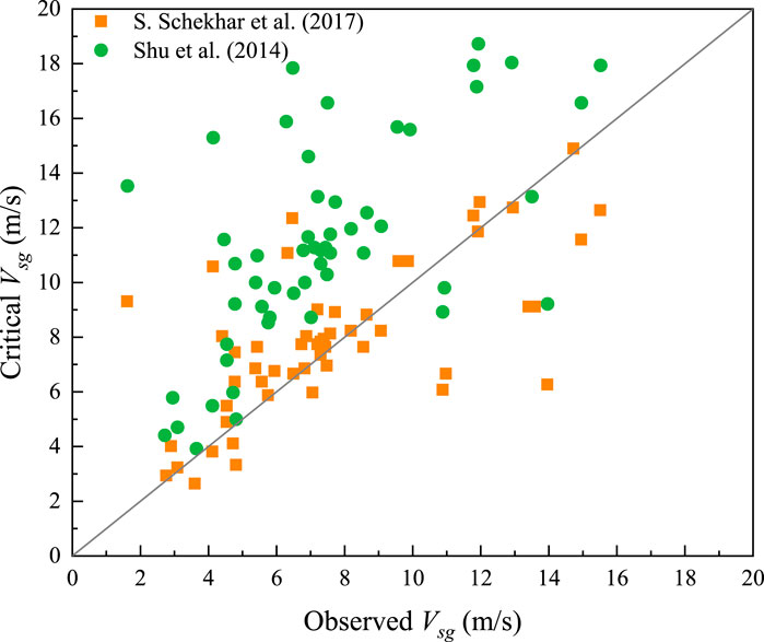
Figure 21. Calculated critical gas velocity vs. measured gas velocity for loading wells studied by Coleman et al. (1991) (Shekhar et al., 2017).

A different equation for the interfacial friction coefficient was incorporated in this study to improve accuracy. This equation accounts for the exposure of a section of the pipe to gas as the liquid film recedes, specifically in the case of an inclined pipe. It is important to note that there is a difference in the friction coefficient between the gas core and the liquid film, compared to the friction coefficient between the gas core and the exposed pipe. By considering this distinction, the prediction of the critical gas velocity and its change with the angle of inclination is improved. The modified critical gas velocity model outperforms other models presented in the existing literature. As the tubing angle changes from vertical to approximately 35°, the liquid film thickness at the top of the pipe tends to approach 0. This reduction in the film thickness is compensated by the increasing thickness at the bottom due to gravitational force. The film profile in the inclined pipe remains relatively unchanged, while the gravitational force continues to decrease beyond 35°. The film thickness reaches the maximum at 35°, and then, the liquid film becomes thinner as the angle increases.

To validate the proposed method, extensive field data were utilized, including some data that had not been reported previously. On the other hand, the approaches proposed by Turner et al. (1969) and Belfroid et al. (2008) are optimistic for large-diameter pipes and inclined wells.

4.2 Fadili model

4.2.1 Theoretical modeling

The new model proposed by Fadili and Shah (2017) introduces the effect of geometric shape changes on the horizontal well flow, especially the effect of droplets on the pipe wall.

This change in wellbore geometry can affect the flow of gas and droplets. After the droplet collides with the wall of the tube, it bounces with a velocity v_b and changes the direction (Figure 22) (Fadili and Shah, 2017).

Figure 22

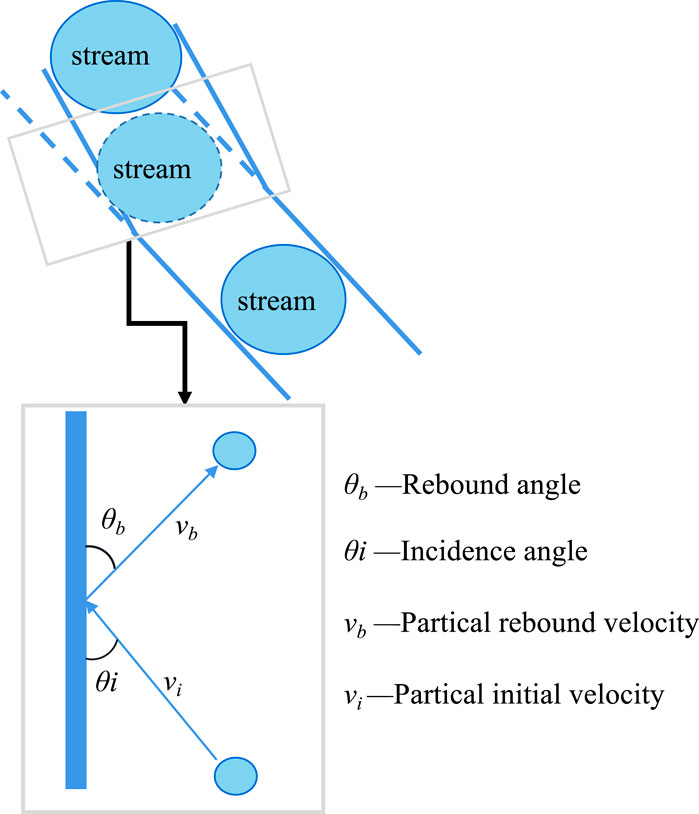
Figure 22. Effect of geometric shape on the droplet rebound impact (Fadili and Shah, 2017).

The droplets are suspended when the gas flow rate is v_c. The gas flow rate under this condition is the critical liquid loading gas flow rate. When the droplet is hit and bounces, it slows down and has a recovery speed v_b lower than v_i. Under the new condition, the droplets at rest will be subjected to the resistance of the gas representing the recovery condition. Then, the droplets will settle. Thus, the “expandable drag” should be built into the initial conditions to counteract this effect so that in the event of a collision, the drag will have no effect on the critical conditions. Droplets settle and accumulate due to the failure of maintaining a critical state.

The energy loss fraction at different incidence angles is calculated to determine the effect of the motion of the droplets after the collision. The revised critical liquid load model Eq. (13) is represented as follows (Fadili and Shah, 2017):

${\mathit{q}}_{\mathit{c}}=\frac{\mathbf{3.067}\times \mathit{P}\times \mathit{A}\times {\mathit{V}}_{\mathit{e}\mathit{f}\mathit{f}}}{\mathit{T}\times \mathit{Z}},(13)$

where $q_c$ is the critical gas rate, $P$ is the pressure, $A$ is the conduit cross-sectional area, $V_{eff}$ is the effective lift velocity, $T$ is the temperature, and $Z$ is the gas compressibility factor.

4.2.2 Model validation in horizontal wells using literature data

The data of some horizontal wells and the actual monitored critical flow rate were provided by Belfroid et al. (2008) and Veeken et al. (2010). The results of the new model are compared with the results of the models provided in the literature.

The accuracy of critical liquid loading production prediction results for 58 gas wells was summarized (Table 7) in the form of absolute mean percentage deviations for each model. The results show that the deviation between the prediction results of the new model established by Fadili and Shah (2017) and the field results is the smallest, i.e., 15.8%. In addition, both Turner and Coleman conventional models underestimated the critical gas content by 24% and 36%, respectively.

Table 7

Table 7. Critical gas rate predictions by four models (Fadili and Shah, 2017).

The data in question are from a study conducted by Belfroid et al. (2008). This study involved observing the critical gas yield of two gas wells and presenting the estimated critical gas yield in a dimensionless form. The ratio between the predicted and actual results of the new model is 1.1 and 0.9, respectively, which is more accurate than the predicted results of Belfroid and Turner. Even though only two wells were used as samples, the new model emerges as the most accurate in predicting critical gas production, outperforming the Belfroid and Turner models.

4.2.3 Experimental work

The field critical gas flow of the horizontal well is measured and compared with the predicted critical gas flow by experiments. The production data of well #1 at different gas flow rates were analyzed to determine the production rate of the gas required to maintain normal production. At a rate of 7.3 million Mscf/d, water and gas production began to show signs of stabilizing. Therefore, the total rate of 730 Mscf/d is the critical rate (Figure 23) (Fadili and Shah, 2017).

Figure 23

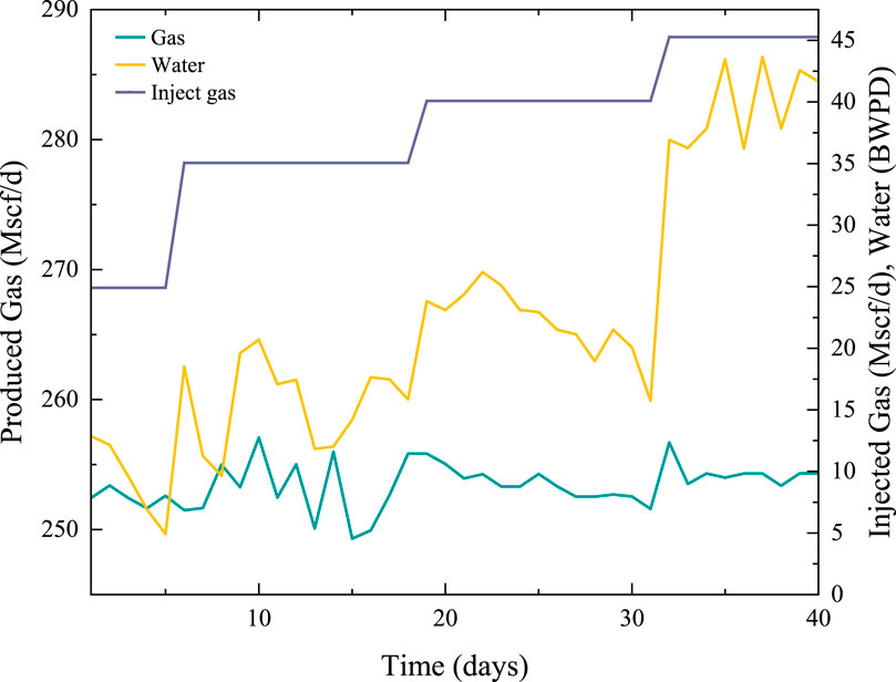
Figure 23. Critical gas rate for horizontal well #1 (Fadili and Shah, 2017).

From the comparison results, the deviation in the vertical well model is too large to be applied to horizontal wells (Table 8) (Fadili and Shah, 2017). In addition, comparing the performance of the new model with that of the horizontal models showed that the new model was significantly better than both at predicting the critical rate.

Table 8

Table 8. Observed critical gas rates and percent deviation for the horizontal well #1 (Fadili and Shah, 2017).

The droplet in the wellbore is caused by the low lift force because the critical gas velocity is not reached. The work by Wallis has been verified, proving that the liquid film will not be produced at high gas velocities. The liquid can be fully loaded. As the speed of the gas decreases, the fluid accumulates to form a thicker film around the core of the gas with entailed droplets. The well will eventually fill up.

A total rate of 684 Mscf/d is considered the critical liquid loading gas rate. The predicted results of each model in well #2 were calculated (Table 9) (Fadili and Shah, 2017). Compared with the vertical models, the new model clearly predicts the critical rate better. In addition, the new model was significantly better than the horizontal models in predicting the critical liquid loading gas rate.

Table 9

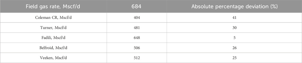
Table 9. Observed critical gas rates and percentage deviation for horizontal well #2 (Fadili and Shah, 2017).

The previous model was mainly applied to vertical wells, while the new model can be applied to horizontal wells and inclined wells. The new model also considers the influence of wellbore geometry on liquid transport. The prediction of the critical liquid loading gas flow rate is more accurate, with a stronger applicability.

In order to improve accuracy and minimize uncertainty in the results, the utilization of correct and accurate PVT data for the specific well was suggested. In addition, in the absence of PVT data, the correlation between the well region and the formation was suggested to be studied.

5 Conclusion

(1) The development potential of deep unconventional gas is huge. The determination of a critical liquid loading model is important for the development of gas reservoirs.

(2) At present, the existing critical liquid carrying models can be divided into mechanism models and semi-empirical models. The model established by Turner is a typical mechanism model, and the models established by Coleman and Veeken are typical semi-empirical models.

(3) Horizontal well hydraulic fracturing technology is widely used in shale gas fields such as the FL shale gas field, WY block, and CN shale gas field. A large amount of the fracturing fluid backflow makes the critical liquid loading model unadaptable when applied. The difference in the type of well causes the difference in where the liquid loads, and the mechanism of establishing the model also changes. The reservoir with low porosity and low permeability is developed by horizontal wells. The inclined segment is more difficult for loading the liquid for the vertical segment and the horizontal segment.

(4) Recent models have been established through new mechanisms. The thickness of the liquid film and the velocity and shape changes of the droplet after collision are considered, and several new models were established. A reasonable modeling mechanism enables models to be applied more accurately.

(5) Under the same angle and liquid quantity condition, the larger the pipe diameter, the higher the critical liquid loading velocity. With the increase in the angle, the thickness of the liquid film under the pipe wall gradually increases, and the wellbore is more likely to produce liquid loading. The larger the liquid velocity is, the larger the critical liquid loading velocity is. The influence of the liquid velocity on the critical liquid loading velocity cannot be ignored. The droplet model is not suitable for the inclined pipe, and the liquid film inversion is the main cause of liquid loading in the inclined pipe.

(6) At present, most of the models do not consider the influence of flow regimes on liquid carrying, and the two-phase flow characteristics of different flow regimes should be considered when establishing new models. More experiments are needed to determine the key parameters in critical liquid loading models.

Author contributions

FH: conceptualization, writing–original draft, and writing–review and editing. XH: investigation, writing–original draft, and writing–review and editing. YY: data curation and writing–review and editing. CB: investigation and writing–review and editing. HX: data curation and writing–review and editing. LP: investigation and writing–review and editing. SZ: visualization and writing–review and editing.

Funding

The author(s) declare that financial support was received for the research, authorship, and/or publication of this article. This work was supported by the Chuanqing Scientific Project (CQZT-yyqxmb-2023-JS-336).

Conflict of interest

Authors FH, XH, YY, CB, HX, and LP were employed by CNPC Chuanqing Drilling Engineering Co., Ltd.

The remaining author declares that the research was conducted in the absence of any commercial or financial relationships that could be construed as a potential conflict of interest.

Publisher’s note

All claims expressed in this article are solely those of the authors and do not necessarily represent those of their affiliated organizations, or those of the publisher, the editors, and the reviewers. Any product that may be evaluated in this article, or claim that may be made by its manufacturer, is not guaranteed or endorsed by the publisher.

References

Alamu, M. B. (2012). Gas-well liquid loading probed with advanced instrumentation. SPE J. 17 (1), 251–270. doi:10.2118/153724-pa

CrossRef Full Text | Google Scholar

Alsaadi, Y. (2013) Liquid loading in highly deviated gas wells. Tulsa: University of Tulsa. Master's thesis.

Google Scholar

Alsanea, M., Mateus-Rubiano, C., and Karami, H. (2022). Liquid loading in natural gas vertical wells: a review and experimental study. SPE Prod. Operations 37, 554–571. doi:10.2118/209819-pa

CrossRef Full Text | Google Scholar

Amaravadi, S., Minami, K., and Shoham, O. (1994). “The effect of pressure on two-phase zero-net liquid flow in inclined pipes,” in SPE Annual Technical Conference and Exhibition, New Orleans, Louisiana, September 1994.

CrossRef Full Text | Google Scholar

Andritsos, N., and Hanratty, T. J. (1987). Interfacial instabilities for horizontal gas-liquid flows in pipelines. Int. J. Multiph. Flow 13 (5), 583–603. doi:10.1016/0301-9322(87)90037-1

CrossRef Full Text | Google Scholar

Barnea, D. (1987). A unified model for predicting flow-pattern transitions for the whole range of pipe inclinations. Intl. J. Multiphas. Flow. 13 (1), 1–12. doi:10.1016/0301-9322(87)90002-4

CrossRef Full Text | Google Scholar

Belfroid, S., Schiferli, W., and Alberts, G. (2008). “Predicting onset and dynamic behavior of liquid loading gas wells,” in Presented at SPE Annual Technical Conference and Exhibition, Denver, 21-24 September, 2008.

Google Scholar

Chen, D., Yao, Ya, Han, H., Fu, G., Song, T., Xie, S., et al. (2016). A new prediction model for critical liquid-carrying flow rate of directional gas wells. Nat. Gas. Ind. 36 (6), 40–44.

Google Scholar

Coleman, B. S. C., Clay, H. B., McCurdy, D. G., and Norris, L. H. (2019). A new look at predicting gas-well load-up. J. Petroleum Technol. 43 (3), 329–333. doi:10.2118/20280-pa

CrossRef Full Text | Google Scholar

Coleman, S. B., Clay, H. B., McCurdy, D. G., and Norris, L. H. (1991). A new look at predicting gas-well load-up. J. Pet. Technol. 43 (3), 329–333. doi:10.2118/20280-pa

CrossRef Full Text | Google Scholar

Fadili, E. F., and Shah, S. (2017). A new model for predicting critical gas rate in horizontal and deviated wells. J. Petroleum Sci. Eng. 150, 154–161. doi:10.1016/j.petrol.2016.11.038

CrossRef Full Text | Google Scholar

Guan, H., Jifei, Yu, Zhou, F., and Weichao, Li (2011). A new method of the critical liquid carrying flow rate for highly deviated gas well. China Offshore Oil Gas 23 (1), 50–52.

Google Scholar

Guner, M. (2012) Liquid loading of gas wells with deviation from 0° to 45°. Tulsa: University of Tulsa. Master's thesis.

Google Scholar

Guo, J., Lu, Q., and He, Y. (2023). Key issues and explorations in shale gas fracturing. Nat. Gas. Ind. B 10 (2), 183–197. doi:10.1016/j.ngib.2023.02.002

CrossRef Full Text | Google Scholar

He, Y., He, Z., Tang, Y., Xu, Y., Xu, J., Li, J., et al. (2023a). Interwell fracturing interference evaluation in shale gas reservoirs. Geoenergy Sci. Eng. 231, 212337. Part A. doi:10.1016/j.geoen.2023.212337

CrossRef Full Text | Google Scholar

He, Y., He, Z., Tang, Y., Xu, Y. J., Long, J. C., and Sepehrnoori, K. (2023b). Shale gas production evaluation framework based on data-driven models. Petroleum Sci. 20 (3), 1659–1675. doi:10.1016/j.petsci.2022.12.003

CrossRef Full Text | Google Scholar

Kvandal, H., Holm, H., and Valle, A. (2007). “Liquid holdup in high pressure, low temperature, gas-condensate flow with low liquid loading including hydrate inhibitor,” in Paper presented at the 13th International Conference on Multiphase Production Technology, Edinburgh, UK, June 2007.

Google Scholar

Li, Li, Lei, Z., Bo, Y., Yin, Y., and Dengwei, Li (2012). Prediction method of critical liquid-carrying flow rate for directional gas wells. OIL GAS Geol. 33 (4).

Google Scholar

Li, R., Chen, Z., Wu, K., and Xu, J. (2023). Shale gas transport in nanopores with mobile water films and water bridge. Petroleum Sci. 20 (2), 1068–1076. doi:10.1016/j.petsci.2022.08.015

CrossRef Full Text | Google Scholar

Liang, W., Wang, J., Leung, C., Goh, S., and Sang, S. (2024). Opportunities and challenges for gas coproduction from coal measure gas reservoirs with coal-shale-tight sandstone layers: a review. Deep Undergr. Sci. Eng. doi:10.1002/dug2.12077

CrossRef Full Text | Google Scholar

Liao, K., Yingchuan, Ll, Yang, Z., and Zhang, H. (2009). Study on pressure drop models of gas-liquid two-phase pipe flow in gas reservoir. ACTA PET. SIN. 30 (4), 607–612.

Google Scholar

Lin, J., Xu, S., and Liu, Y. (2023). Experimental and modeling studies on continuous liquid removal in horizontal gas wells. Front. Earth Sci. 11. doi:10.3389/feart.2023.1288208

CrossRef Full Text | Google Scholar

Liu, Y. (2019) Study on drainage and production technology of CN shale gas horizontal wells. Master's thesis. Southwest Petroleum University.

Google Scholar

Liu, Y., Dou, Z., Yang, G., Chen, Z., and Gao, D. (2023a). A designing method of infill wells bypass trajectory in fracturing domains of shale gas fields. Geoenergy Sci. Eng. 230, 212188. doi:10.1016/j.geoen.2023.212188

CrossRef Full Text | Google Scholar

Liu, Z. L., Liu, L., Fang, Y. Z., and Liao, R. Q. (2023b). A new prediction model for the critical gas velocity of liuid-carryng in horizontal gas wells. J. Yangtze Univ. Nat. Sci. Ed. 20 (2).

Google Scholar

Luo, N., Zhang, H., Chai, Y., Li, P., Zhai, C., Zhou, J., et al. (2023). Research on damage failure mechanism and dynamic mechanical behavior of layered shale with different angles under confining pressure. Deep Undergr. Sci. Eng. 2 (4), 337–345. doi:10.1002/dug2.12063

CrossRef Full Text | Google Scholar

Meng, J., Zhou, Y. J., Ye, T. R., Xiao, Y. T., Lu, Y. Q., Zheng, A. W., et al. (2023). Hybrid data-driven framework for shale gas production performance analysis via game theory, machine learning, and optimization approaches. Petroleum Sci. 20 (1), 277–294. doi:10.1016/j.petsci.2022.09.003

CrossRef Full Text | Google Scholar

Min, L. I., Guo, P., and Guangtian, T. A. N. (2001). New look on removing liquids from gas wells. Petroleum Explor. Dev. 28 (5), 105–106.

Google Scholar

Min, L. I., Pin, G. U. O., Zhang, M., Mei, H. Y., Liu, W., Li, S. L., et al. (2002). Comparative study of two models for continuous removal of liquids from gas wells. J. Southwest Petroleum Inst. 24 (4), 30–32.

Google Scholar

Na, W., Yinchuan, Li, and Yueqin, Li (2007). Visual experimental research on gas well liquid loading. DRLLING Prod. Technol. 30 (3), 43–45.

Google Scholar

Nie, J., Qiao, L., Wang, B., Wang, W., Li, M., and Zhou, C. (2023). Prediction of dynamic liquid level in water-producing shale gas wells based on liquid film model. Front. Earth Sci. 11. doi:10.3389/feart.2023.1230470

CrossRef Full Text | Google Scholar

Pagou, L., and Wu, X. (2020). “Liquid film mode for prediction and identification of liquid loading in vertical gas wells,” in Paper presented at the International Petroleum Technology Conference, Dhahran, Kingdom of Saudi Arabia, January 2020.

Google Scholar

Pan, L., and Hanratty, T. J. (2002). Correlation of entrainment for annular flow in horizontal pipes. Int. J. Multiph. Flow 28 (3), 385–408. doi:10.1016/s0301-9322(01)00074-x

CrossRef Full Text | Google Scholar

Qian, Z., Shuqiang, S., and Yimin, W. (2022). Diagnosis and model comparison of liquid loading in deep shale gas horizontal wells. Technol. Appl. Res. Mod. Chem. Res., 64–66.

Google Scholar

Rodrigues, H. T., Pereyra, E., and Cem, S. (2019). Pressure effects on low-liquid-loading oil/gas flow in slightly upward inclined pipes: flow pattern, pressure gradient, and liquid holdup. SPE J. 24, 2221–2238. doi:10.2118/191543-pa

CrossRef Full Text | Google Scholar

Shekhar, S., Kelkar, M., Hearn, W. J., and Hain, L. L. (2017). Improved prediction of liquid loading in gas wells. SPE Prod. Operations 32 (4), 539–550. doi:10.2118/186088-pa

CrossRef Full Text | Google Scholar

Shi, J. T., Jia, Y. R., Zhang, L. L., Ji, C. J., Li, G. F., Xiong, X. Y., et al. (2022). The generalized method for estimating reserves of shale gas and coalbed methane reservoirs based on material balance equation. Petroleum Sci. 19 (6), 2867–2878. doi:10.1016/j.petsci.2022.07.009

CrossRef Full Text | Google Scholar

Shu, L., Kelkar, M., Pareyra, E., and Sarica, C. (2014). A new comprehensive model for predicting liquid loading in gas wells. SPE Prod Oper 29 (4), 337–349. doi:10.2118/172501-pa

CrossRef Full Text | Google Scholar

Taitel, Y., and Dukler, A. E. (1976). A model for predicting flow regime transitions in horizontal and near horizontal gas-liquid flow. Aiche J. 22 (1), 47–55. doi:10.1002/aic.690220105

CrossRef Full Text | Google Scholar

Turner, R. G., Hubbard, M. G., and Dukler, A. E. (1969). Analysis and prediction of minimum flow rate for the continuous removal of liquids from gas wells. J. PETROLEUM Technol. 21 (11), 1475–1482. doi:10.2118/2198-pa

CrossRef Full Text | Google Scholar

Veeken, K., Hu, B., and Schiferli, W. (2010). Gas-well liquid-loading field-data analysis and multiphase-flow modeling. SPE Prod Oper 25 (3), 275–284. doi:10.2118/123657-pa

CrossRef Full Text | Google Scholar

Wang, Z. B., Guo, L. J., Zhu, S. Y., and Nydal, O. J. (2017). Prediction of the critical gas velocity of liquid unloading in a horizontal gas well. SPE J. 23 (2), 328–345. doi:10.2118/189439-pa

CrossRef Full Text | Google Scholar

Wang, J., Jia, A., He, D., Yunsheng, W. E. I., and Qi, Y. (2014b). Rate decline of multiple fractured horizontal well and influence factors on productivity in tight gas reservoirs. Nat. Gas. Geosci. 25 (2), 278–285.

Google Scholar

Wang, J., Jia, A., Yunsheng, W. E. I., and Zhao, W. (2016). Pseudo steady productivity evaluation and optimization for horizontal well with multiple finite conductivity fractures in gas reservoirs. J. China Univ. Petroleum 40 (1), 100–106.

Google Scholar

Wang, J., Yan, C., Jia, A., He, D. b., Wei, Y. s., and Qi, Y. d. (2014a). Rate decline analysis of multiple fractured horizontal well in shale reservoir with triple continuum. J. Central South Univ. 21 (11), 4320–4329. doi:10.1007/s11771-014-2431-4

CrossRef Full Text | Google Scholar

Wang, X., Zhang, S., Qi, W. U., Liu, Y. Z., and Lei, Q. (2009). Factors affecting the productivity of multi-section fractures in subsection fracturing of horizontal wells. OILDRILLING Prod. Technol. 31 (1), 73–76.

Google Scholar

Wang, Y., Dong, D., and Jianzhong, L. I. (2012). Reservoir characteristics of shale gas in longmaxi formation of the lower silurian, southern sichuan. ACTA PET. SIN. 33 (4), 551–561.

Google Scholar

Wang, Y., and Liu, Q. (2007). A new method to calculate the minimum critical liquids carrying flow rate for gas wells. P. G. O. D. D. 26 (6), 82–85.

Google Scholar

Wenying, Li (2015a). The research of prediction on critical liquid carrying model for horizontal wells. Oil Prod. Eng. Collect. 4, 72–75.

Google Scholar

Wenying, L. I. (2015b). The research of prediction on critical liquid carrying model for horizontal wells. OIL Prod. Eng. 4, 72–82.

Google Scholar

Williams, L. R., Dykhno, L. A., and Hanratty, T. J. (1996). Droplet flux distributions and entrainment in horizontal gas-liquid flows. Int. J. Multiph. Flow 22 (1), 1–18. doi:10.1016/0301-9322(95)00054-2

CrossRef Full Text | Google Scholar

Xiangdong, Y. U., Shuqiang, S. H. I., Guoliang, Ll, Fang, J. W., and Duan, C. L. (2024). Research on critical liquid loading model for directional wells based on liquid film inversion. Petroleum Reserv. Eval. Dev. 14 (1), 151–158.

Google Scholar

Xianting, A. I. (2019) Prediction model of critical gas velocity in horizontal gas well. Master's thesis. South west Petroleum University Engineering.

Google Scholar

Xiao, G., and Yingchuan, Li (2010). Theory and experiment on the continuous liquid carrying in horizontal wells. J. Oil Gas Technol. 32 (1), 324–327.

Google Scholar

Yang, W., Ming, WANG, Qiumeng, ZHOU, Yuele, J. I. A., and Liang, CHEN (2009). A NEW METHOD AND THE APPLICATON OF PREDICTNG CRITICAL LIQUID CARRYING RATE IN GAS WELL. J. Southwest Petroleum Univ. Sci. Technol. Ed. 31 (6).

Google Scholar

Yunsheng, W., Qi, Y., Jia, C., Jin, Y., and He, Y. (2019). Production performance of and development measures for typical platform horizontal wells in the WY Shale Gas Field, Sichuan Basin. Nat. Gas. Ind. 39 (1), 81–86.

Google Scholar

Yunyang, G. (2021). Determination and application of critical liquid loading model in ZJ gas field. Enterp. Technol. Dev. 7, 43–45.

Google Scholar

Zhang, X., Li, H., Tan, X., Li, G., and Jiang, H. (2023). Coupling effects of temperature, confining pressure, and pore pressure on permeability and average pore size of Longmaxi shale. Deep Undergr. Sci. Eng. 2 (4), 359–370. doi:10.1002/dug2.12047

CrossRef Full Text | Google Scholar

Zhao, S., and Liu, C. (2019). The new calculation model of critical liquid carrying flow rate in FL gas field. Yunnan Chem. Technol. 46 (5), 167–170.

Google Scholar

Zhao, Q., Wang, H., Lianzhu, CONG, Zhang, Q., and Zou, Z. (2023). Shale gas resources/reserves calculation method considering the space taken by adsorbed gas. Nat. Gas. Geosci. 34 (2), 326–333.

Google Scholar

Zhao, Y. (2019). Research and application of foam drainage technology in horizontal wells. Southwest Pet. Univ. Eng. Master's thesis.

Google Scholar

Zheng, J., Changhui, Y., Zhang, W., Zheng, F., and Xu, W. F. (2011). Study on minimum liquid-carrying production of gas producer in DND gas field. PGRE 18 (1), 70–33.

Google Scholar

Zhou, J., Yi, L. U. O., Yingchuan, Ll, Zhong, H., and Zhou, R. (2013). A model to calculate liquid - carrying critical flow rate for horizontal wells in DND gas field. J. Chongqing Univ. Sci. Technol. Nat. Sci. Ed. 15 (2), 67–71.

Google Scholar