Complex fracture description and quasi-elastic energy development mathematical model for shale oil reservoirs

Reservoir numerical simulation is an important tool and method for the reasonable and efficient development of shale reservoirs. Accurate description of three-dimensional fractures in shale reservoir development is a necessary and sufficient condition to improve the accuracy and robustness of shale reservoir numerical simulation. This paper achieves precise characterization of complex fracture shapes and oil, gas and water flow by establishing an embedded discrete fracture model based on a non-structural network, which has advantages in the fine characterization of complex morphological fractures in the reservoir and the grid division of the reservoir. In the large matrix solution method, the Newton-Raphson method is used to linearize the nonlinear equations, the Jacobian matrix is ​​constructed, the ILU method is used for preprocessing, the conjugate gradient method is used to solve the linear equations, and the shale oil quasi-elasticity is established A fully implicit solution method for mathematical models of energy development.

1 Introduction

China’s continental shale formations are rich in huge shale oil resource potential, with diverse lithofacies, frequent phase changes, developed bedding fractures, and strong heterogeneity. In view of the characteristics of shale oil reservoirs with low permeability and low porosity, which are difficult to be exploited through conventional development methods, hydraulic fracturing is usually used to reform the reservoir first and then develop it. Therefore, for shale oil reservoirs, whether they are artificial fractures or natural fractures, the development of fractures has become a key technical issue. Naturally, in recent years, domestic and foreign scholars have focused their research on the laws and mechanisms of crack development and expansion (Meng, 2024). Hou Bing et al. conducted an indoor true triaxial indoor fracturing physical simulation experiment and used concrete to wrap a full-diameter downhole core to test the initiation and vertical extension of hydraulic fractures in a true triaxial environment, thereby explaining the Chang 7 shale of the Yanchang Formation in the Ordos Basin. The vertical propagation mechanism of oil reservoir fracturing cracks (Zou et al., 2022). Numerical simulation is an important tool for predicting and evaluating shale reservoir development effects. Whether it can accurately describe the three-dimensional fracture diffusion model is the key to the accuracy of the numerical simulation results of shale reservoirs. Wang Yizhao et al. established a shale oil multi-layered pseudo-three-dimensional fracture propagation model based on the finite element method (Wang et al., 2021). Hou Bing et al. established a three-dimensional discrete element model of dense-cut fracturing fracture propagation and studied the competitive expansion rules of multi-cluster fractures (Zhang et al., 2021). Zhu Haiyan et al. established a three-dimensional seepage-stress-damage model for the dynamic expansion of multiple fractures in horizontal wells (Hou et al., 2022).

However, how to accurately characterize multi-scale fractures in numerical simulations and improve the accuracy of numerical simulations of shale reservoirs is still a problem that needs to be solved. Existing shale oil and gas numerical simulation models mainly include dual media, multiple discrete media, and equivalent media. Among them, dual media is the most widely used because of its balance between calculation accuracy and speed (Chen et al., 2018).

Current numerical simulations of reservoirs generally require the establishment of explicit fractures in the matrix grid system. Structured grids and unstructured grids are the two most commonly used grid types in reservoir numerical simulation. Because describing complex fractures often requires meshing to describe complex shapes and arbitrary connected areas, it is difficult for structured grids to achieve a precise description of this problem. Therefore, this article chooses to use unstructured grids for processing. The modeling process needs to consider the arrangement of fracture grids and matrix grids at the same time, which cannot satisfy the simulation of complex structural and morphological fractures. Triangular grids are conventionally used to describe fracture grids because the fluid flow direction is not perpendicular to the grid edges. When calculating parameters such as conductivity and circulation, it is necessary to calculate the angle between the flow direction and the grid edge lines to obtain the fluid flow through the grid. actual volume. Therefore, it has certain disadvantages compared with PEBI grid in terms of calculation accuracy and efficiency. The orthogonality between the flow direction of the PEBI grid and the grid lines determines that the fluid is considered to flow along the connections between grid nodes during the numerical simulation calculation process. On the other hand, since the width of cracks is usually on the millimeter or centimeter level, in order to explicitly characterize the crack morphology, current simulation methods generally use the method of overall grid densification or local grid densification to transition from the large-scale grid of the matrix to The small-scale grid of cracks has too many grids after densification. Many simulations can only use the good symmetry of the radial grid to reduce the number of grids to achieve effective simulations, and a large number of minimization grids are generated during calculations, resulting in poor calculation convergence (Mirzaei and Cipolla, 2012; Zhao et al., 2018). Therefore, the current grid characterization technology cannot meet the needs of large-scale complex fractured shale reservoir simulation.

This paper uses an embedded discrete fracture model based on a non-structural network to accurately represent complex fracture shapes and gas and water flows. The PEBI non-structured grid with good local orthogonality is used for fracture characterization. At the same time, a PEBI non-structured grid adaptive local refinement partitioning method is established, which is better adapted to the fine characterization of complex-shaped fractures in the reservoir and the reservoir grid. divide.

Because shale oil reservoir development is mostly based on reservoir stimulation methods such as fracturing, the pressure within the well control range will be slightly higher than the formation pressure within a certain period of time. Therefore, it is different from traditional elastic energy development, taking into account factors such as starting pressure gradient and stress sensitivity, a mathematical model for quasi-elastic energy shale reservoir development was constructed. In terms of solution, the Newton-Raphson method is used to linearize the nonlinear equation, the Jacobian matrix is ​​constructed, the ILU method is used for preprocessing, the conjugate gradient method is used for matrix solving, and a mathematical model of shale oil quasi-elastic energy development is established. Fully implicit solution method.

2 Complex fracturing modeling

2.1 Grid modeling

The PEBI grid is an unstructured local orthogonal grid (Figure 1). It is more flexible than the structured grid and can well simulate the boundaries of irregular geological bodies and facilitate local refinement; at the same time, it satisfies the finite difference method. Due to the requirement of grid orthogonality, the final difference equation is similar to the Cartesian grid finite difference method. During the calculation process, it is not necessary to calculate the actual flux of the fluid through reduced projection. Therefore, in the field of reservoir numerical simulation, the PEBI grid and the radial grid form a hybrid grid, which can avoid over-density of the grid and improve the stability and speed of numerical calculations.

Figure 1

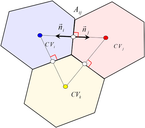
Figure 1. PEBI local orthogonal grid system schematic.

PEBI meshing adopts the method of first laying out mesh nodes and then dividing the mesh. Therefore, the quality of the point distribution algorithm determines the quality of the meshing. This further affects the stability and speed of simulation calculations. When selecting grid nodes, this paper gives four limiting conditions from points, lines, domains, and surfaces, so as to obtain reasonable grid nodes. When distributing grid nodes in the simulation area, the following restrictions must be met.

1. Restricted point: The given point must become a PEBI grid node.

2. Limiting line: The grid must be distributed along the given polyline, and grids crossing the limiting line are not allowed.

3. Limited domain: Grids cannot appear within the internal limited domain, and grids cannot appear outside the external limited domain.

4. Limited surface: A small surface of the grid block must be on a given plane piece, and grids that span the limited surface are not allowed.

Due to the complex changes in the positional relationship between boundaries and wells, the correctness of the grid must be ensured through the distribution of grid nodes. Use boundary, well and other information to divide the reservoir into several sub-areas, and then distribute grid nodes on the sub-areas so that the distributed grid nodes meet the limiting conditions in the sub-areas and different areas are independent of each other. Then these mesh nodes are subjected to Delaunay triangulation and Vornoni meshing, and finally the PEBI mesh is obtained after removing the invalid meshes.

2.2 Fracturing representation model

Actual shale reservoirs are highly heterogeneous and multi-scale, and fractures have significant multi-scale characteristics. Current methods for characterizing and simulating fractures mainly include grid refinement method, dual-pore and dual-permeability characterization method, and discrete fracture method. Among them, the grid densification method characterizes cracks through local or global grid densification. However, since the width of cracks is usually in the millimeter-centimeter level, and the width of the matrix grid is often in the meter level, the grid densification method is used to characterize the cracks. Refinement of the matrix grid to the fracture scale will easily lead to too many grids and excessive calculations. At the same time, the grid densification method makes it difficult to accurately depict complex fracture morphology.

The dual-pore dual-permeability model simplifies the fracture topology information, assumes that there are uniformly distributed fractures around the matrix unit, and represents the difference in fracture properties (density, etc.) through the heterogeneous conductivity of the fracture grid. The dual-pore dual-permeability model is commonly used for flow simulation in reservoirs with a large number of natural fractures. However, for reservoirs with strong heterogeneity, complex fracture structures and poor connectivity, the model accuracy is low.

The discrete fracture model is a model with fully explicit representation of fractures, which can accurately represent the behavior and influence of fractures. When dealing with complex fracture seepage problems, the discrete model with explicit representation of fractures is more suitable. Discrete fracture network simulation can directly use the information of discrete fractures to simulate, and can capture the topology of fractures in fine detail. The discrete crack model can be further divided into a representation method based on unstructured grids and an embedded discrete crack representation method based on structured grids (Figure 2). The calculation results of the characterization method based on unstructured grids are more accurate, but not The division of structural mesh is more difficult. In the embedded discrete crack representation method, the crack direction does not affect the grid modeling, but due to the cutting between the cracks and the grid, its calculation accuracy is relatively low.

Figure 2

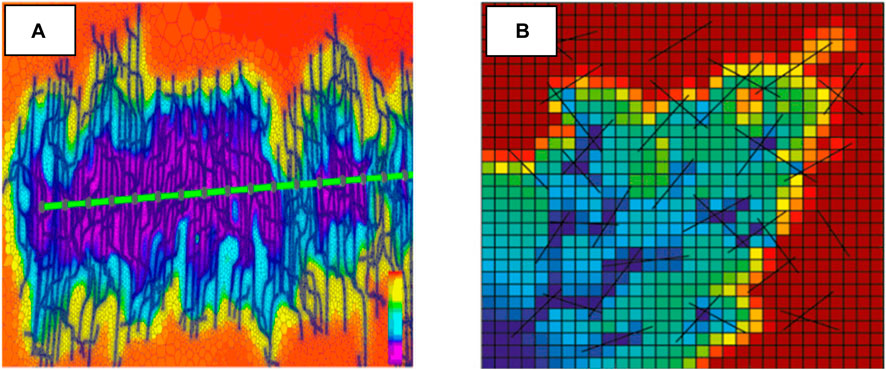
Figure 2. (A) Discrete crack characterization method (B) Embedded discrete crack characterization method.

In order to improve the simulation accuracy, this paper adopts a discrete crack characterization method based on unstructured grids. Currently commonly used unstructured grids include triangular grids and PEBI grids. The PEBI unstructured grid has better local orthogonality, so there is no need for flux projection when calculating matrix-fracture and matrix-matrix mass exchange. Compared with the simulation method based on triangular grids, it is more robust and can achieve accurate characterization of complex fracture shapes (Figure 3) and gas and water flows. Therefore, this paper uses PEBI unstructured grids to carry out subsequent simulation research.

Figure 3

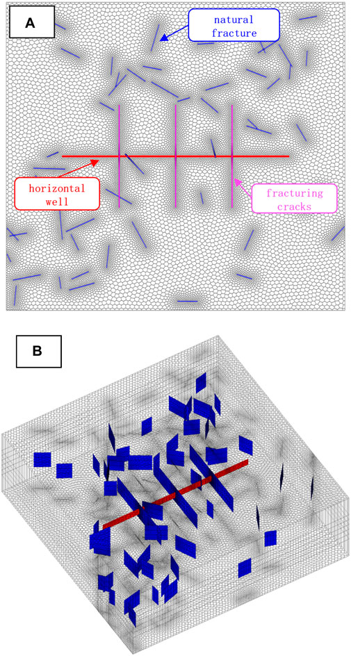
Figure 3. (A) Planar grid diagram based on discrete crack and PEBI unstructured grid (B) 3D grid diagram based on discrete crack and PEBI unstructured grid.

For shale reservoirs, a large number of microseismic monitoring results show that the fractures generated after hydraulic fracturing are not simple long straight fractures, but complex fracture networks with a large number of secondary fractures (Figure 4A). The PEBI non-structural meshing method established in this article has the ability of adaptive local refinement. As the complexity of the fracture shape increases, the grid node selection will follow the fracture shape, which can be better adapted to the fine characterization and delineation of complex shape fractures in the reservoir. Reservoir meshing (Figure 4B).

Figure 4

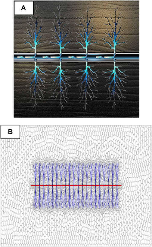
Figure 4. (A) Complex fractures after hydraulic fracturing (B) Modeling of complex hydraulic fracture morphology.

3 Cross fracturing modeling

The discrete fracture model requires the use of non-structural grids to mesh the simulation space, which can meet the needs of complex cross-crack modeling (Figure 5). However, when solving the model, the volume of the fracture needs to be considered, and then the fracture and the Mass and energy exchange between matrix and cracks. The flow between matrix and matrix, between cracks and matrix, and between cracks is assumed to satisfy Darcy’s seepage law, so the seepage velocity can be calculated according to the following formula Eq. (1):

$\overrightarrow{{\mathrm{\nu }}_{\mathrm{\beta }}}=-\frac{{\mathrm{\rho }}_{\mathrm{\beta }}{\mathrm{k}}_{\mathrm{r}\mathrm{\beta }}}{\mathrm{A}{\mathrm{\mu }}_{\mathrm{\beta }}}\mathrm{T}\Delta \left({\mathrm{p}}_{\mathrm{\beta }}-{\mathrm{\rho }}_{\mathrm{\beta }}\text{gD}\right)(1)$

Figure 5

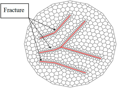
Figure 5. Fracture grid division schematic.

In the formula, ${\mathrm{\rho }}_{\mathrm{\beta }}$ is the density of β phase, kg/m³, ${\mathrm{k}}_{\mathrm{r}\mathrm{\beta }}$ is the relative permeability of β phase; A is the cross-sectional area, m², ${\mathrm{\mu }}_{\mathrm{\beta }}$ is the viscosity of β phase, Pa.s, T is the conductivity, m³, ${\mathrm{p}}_{\mathrm{\beta }}$ is the pressure of β phase, Pa, g is the gravity acceleration, m/s²; D is the depth, m.

The discrete fracture model contains three types of connection relationships between matrix and matrix, between matrix and cracks, and between cracks and cracks. Among them, the connection between cracks and cracks is relatively complex, which includes both as shown in Figure 6A The connection between two cracks (Ω₁ and Ω₂). At the same time, when multiple cracks intersect, they will also face the connection between multiple cracks (Ω₁, Ω₂, Ω₃) as shown in Figure 6B There is a connection situation. Karimi-Fard et al. studied the various connection relationships mentioned above. They introduced an interface control volume (Ω₀) at the fracture junction for processing, eliminated Ω₀, and then obtained n grid units (matrix or cracks). The general formula for conductivity during connection is Eq. (2):

$\left\{\begin{array}{l}\mathrm{T}=\frac{{\mathrm{\alpha }}_{\mathrm{i}}{\mathrm{\alpha }}_{\mathrm{j}}}{{\displaystyle \sum _{\mathrm{k}=1}^{\mathrm{n}}}{\mathrm{\alpha }}_{\mathrm{k}}}\\ {\mathrm{\alpha }}_{\mathrm{k}}=\frac{{\mathrm{A}}_{\mathrm{k}}{\mathrm{k}}_{\mathrm{k}}}{{\mathrm{D}}_{\mathrm{k}}}\underset{{\mathrm{n}}_{\mathrm{k}}}{\to }\bullet \underset{{\mathrm{f}}_{\mathrm{k}}}{\to }\end{array}\right.(2)$

Figure 6

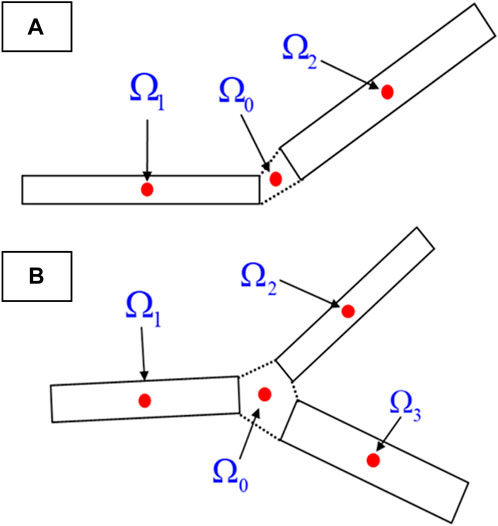
Figure 6. (A) Cross of two fracture (B) Multiple fracture intersection.

In the formula, A_k is the area of the kth grid connection surface, m²; k_k is the permeability of the kth grid, m²; D_k is the distance between the center point of the connection surface and the kth grid center point, m; $\underset{{\mathrm{n}}_{\mathrm{k}}}{\to }$ is the unit normal vector of the kth grid connection surface; $\underset{{\mathrm{f}}_{\mathrm{k}}}{\to }$ is the unit vector between the center point of the connection surface and the kth grid center point.

The above formula shows that when two fractures intersect, the calculation of the conductivity is only related to the attribute values ​​​​of the two connected fractures, but when multiple fractures intersect, the conductivity between the two fractures is related to all connected fractures. Related to the attribute value.

4 Establishment of a fully implicit solution method for the development of shale oil quasi-elastic energy model

The fully implicit solution method for the mathematical model of quasi-elastic energy development of shale oil was established by linearizing nonlinear equations using the Newton-Raphson method, constructing the Jacobian matrix, preprocessing with the ILU method, and solving the matrix using the conjugate gradient method.

(1) Mathematical Model Discretization

The equation of mass conservation for the three components of oil, gas, and water can be written in the following form Eq. (3):

$\frac{\partial M^{\kappa }}{\partial t}+\nabla \cdot {\overrightarrow{F}}^{\kappa }=q^{\kappa }(3)$

The integral form of the above equations, derived using the finite difference method, is as follows Eq. 4:

$\frac{d}{dt}{\displaystyle \underset{V_n}{\int }}{M}^{\kappa }dV={\displaystyle \underset{S_n}{\int }}{F}^{\kappa }ndS+{\displaystyle \underset{V_n}{\int }}{q}^{\kappa }dV(4)$

In the equation, M presents the momentum of the fluid at temperature k per unit time; F represents the force at temperature k; ${\mathrm{V}}_{\mathrm{n}}$ represents the volume of any nth micro unit; dV represents the micro unit within this unit; S_n represents the outer surface area of any nth micro unit; dS represents the micro area on the surface of this unit; n represents the unit normal vector on the surface of the micro unit (if the external normal is taken as negative) (Figure 7).

Figure 7

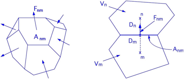
Figure 7. Schematic of finite volume discretization.

For the nth discrete unit, the volume average yields Eqs (5), (6):

${\displaystyle \underset{V_n}{\int }}{M}^{\kappa }dV=M_n^{\kappa }{V}_n(5)$

${\displaystyle \underset{V_n}{\int }}{q}^{\kappa }dV=q_n^{\kappa }{V}_n(6)$

In the equation, $M_n^{\kappa }$ and $q_n^{\kappa }$ represents the average value of M^K and q^K in the nth unit.

For the nth unit adjacent to many other units 1,2,3, etc., let’s assume any unit is denoted as m. The interface area between the mth and nth units is denoted as A_mn The average value of F_k along the normal direction within the interface between unit n and unit m is denoted as $F_{nm}^{\kappa }$. Then, for the nth unit Eq. 7:

${\displaystyle \underset{S_n}{\int }}{F}^{\kappa }\cdot ndS={\displaystyle \sum _m}{A}_{nm}{F}_{nm}^{\kappa }(7)$

This leads to the spatial discretization form of the control equation as follows Eq. (8):

$\frac{d{M}_n^{\kappa }}{dt}=\frac{1}{V_n}{\displaystyle \sum _m}{A}_{nm}{F}_{nm}^{\kappa }+q_n^{\kappa }(8)$

Based on first finite differencing, the discretization of time is performed. To ensure stability, the fluxes and source-sink terms are treated using a fully implicit method Eq. (9):

$\frac{M_{n,t+\Delta t}^{\kappa }-M_{n,t}^{\kappa }}{\Delta t}=\frac{1}{V_n}{\displaystyle \sum _m}{A}_{nm}{F}_{nm,t+\Delta t}^{\kappa }+q_{n,t+\Delta t}^{\kappa }(9)$

Defining the residual as the difference between the left and right sides of the above equation, we have Eq. (10):

$R_{n,t+\Delta t}^{\kappa }=M_{n,t+\Delta t}^{\kappa }-M_{n,t}^{\kappa }-\frac{\Delta t}{V_n}{\displaystyle \sum _m}{A}_{nm}{F}_{nm,t+\Delta t}^{\kappa }-\Delta t{q}_{n,t+\Delta t}^{\kappa }=0(10)$

(2) Mathematical Model Solution

Unit i: Oil, gas, and water, with primary variables x_i,1 (po), x_i,2 (po), x_i,3 (po). The nonlinear equations within unit i are Eq. (11):

$\left\{\begin{array}{c}{f}_{i,1}=M_{i,t+\Delta t}^o-M_{i,t}^o-\frac{\Delta t}{V_i}{\displaystyle \sum _n}{A}_{in}{F}_{in,t+\Delta t}^o-\Delta t{q}_{i,t+\Delta t}^o=0\\ f_{i,2}=M_{i,t+\Delta t}^g-M_{i,t}^g-\frac{\Delta t}{V_i}{\displaystyle \sum _n}{A}_{in}{F}_{in,t+\Delta t}^g-\Delta t{q}_{i,t+\Delta t}^g=0\\ f_{i,3}=M_{i,t+\Delta t}^w-M_{i,t}^w-\frac{\Delta t}{V_i}{\displaystyle \sum _n}{A}_{in}{F}_{in,t+\Delta t}^w-\Delta t{q}_{i,t+\Delta t}^w=0\end{array}\right.(11)$

Unit j: Oil, gas, and water, with primary variables x_j,1 (po), x_j,2 (po), x_j,3 (po). The nonlinear equations within unit j are Eq. (11):

$\left\{\begin{array}{c}{f}_{j,1}=M_{j,t+\Delta t}^o-M_{j,t}^o-\frac{\Delta t}{V_j}{\displaystyle \sum _n}{A}_{jn}{F}_{jn,t+\Delta t}^o-\Delta t{q}_{j,t+\Delta t}^o=0\\ f_{j,2}=M_{j,t+\Delta t}^g-M_{j,t}^g-\frac{\Delta t}{V_j}{\displaystyle \sum _n}{A}_{jn}{F}_{jn,t+\Delta t}^g-\Delta t{q}_{j,t+\Delta t}^g=0\\ f_{j,3}=M_{j,t+\Delta t}^w-M_{j,t}^w-\frac{\Delta t}{V_j}{\displaystyle \sum _n}{A}_{jn}{F}_{jn,t+\Delta t}^w-\Delta t{q}_{j,t+\Delta t}^w=0\end{array}\right.(12)$

f_i,1 is not only a function of its own primary variables x_i,1, x_{i, 2}, x_i,3, but also a function of the primary variables x_m,1, x_m,2, x_m,3 of adjacent units m (1,2 … ), due to the fluid flow between adjacent units:

The forms of units i and j in the system of equations (3N nonlinear equations) are Eqs (13), (14):

$\left\{\begin{array}{c}⋮\\ f_{i,1}=f_{i,1}\left(\dots x_{i,1},x_{i,2},x_{i,3}\dots x_{j,1},x_{j,2},x_{j,3}\dots \right)\\ f_{i,2}=f_{i,1}\left(\dots x_{i,1},x_{i,2},x_{i,3}\dots x_{j,1},x_{j,2},x_{j,3}\dots \right)\\ f_{i,3}=f_{i,3}\left(\dots x_{i,1},x_{i,2},x_{i,3}\dots x_{j,1},x_{j,2},x_{j,3}\dots \right)\\ ⋮\end{array}\right.(13)$

$\left\{\begin{array}{c}⋮\\ f_{j,1}=f_{j,1}\left(\dots x_{i,1},x_{i,2},x_{i,3}\dots x_{j,1},x_{j,2},x_{j,3}\dots \right)\\ f_{j,2}=f_{j,1}\left(\dots x_{i,1},x_{i,2},x_{i,3}\dots x_{j,1},x_{j,2},x_{j,3}\dots \right)\\ f_{j,3}=f_{j,3}\left(\dots x_{i,1},x_{i,2},x_{i,3}\dots x_{j,1},x_{j,2},x_{j,3}\dots \right)\\ ⋮\end{array}\right.(14)$

Using the Newton-Raphson iteration method to solve the system of multivariable nonlinear equations, considering an n-element nonlinear equation system Eq. (15):

$f\left(x\right)=0(15)$

As:

$f=\left[\begin{array}{c}{f}_1\left(x_1,x_2\cdots x_n\right)\\ f_2\left(x_1,x_2\cdots x_n\right)\\ \cdots \\ f_n\left(x_1,x_2\cdots x_n\right)\end{array}\right]=\left[\begin{array}{c}0\\ 0\\ \cdots \\ 0\end{array}\right](16)$

Expanding the Taylor series at x and taking the linear part Eq. (17):

$f\left(x+\Delta x\right)=f\left(x\right)+J\left(x\right)\Delta x(17)$

The Jacobian matrix, J(x) of size n×n, represents the first-order partial derivatives of the multivariable function arranged in a certain order, with elements given by:

$J_{ij}=\frac{\partial f_i}{\partial x_j}(18)$

Analytical derivatives are generally difficult to obtain, so we use finite difference method:

$\frac{\partial f_i}{\partial x_j}\approx \frac{f_i\left(x_j+10^{-8}{x}_j\right)-f_i\left(x_j\right)}{10^{-8}{x}_j}(19)$

Assuming x is the current approximate solution and x+∆x is the next approximate solution, such that f (x+∆x) = 0, we can derive the equation for ∆x from Eq. 19:

$\Delta x=-{\left[J\left(x\right)\right]}^{-1}f\left(x\right)(20)$

The calculation steps are as follows.

1. Decompose the matrix using the ILU method to obtain a sparse matrix.

2. Use the CG (Conjugate Gradient) algorithm for iterative solution.

3. Estimate an initial value x.

4. Let f (x+∆x) = 0 and enter Eq. 16 to calculate f(x).

5. Use Eq. 18 to calculate $\mathrm{J}\left(\mathrm{x}\right)$.

6. Substitute steps 4 and 5 into Eq. 20 to calculate ∆x.

7. Let xnew←xold+∆x, repeat steps 4-7 until the error is less than the error precision, that is, |∆x |<ε.

The Jacobian matrices of the i and j unit nonlinear equation systems are respectively Eqs (21), (22):

$\left[\begin{array}{ccccccccc}⋮& & & & & & & & \\ \cdots & \frac{\partial f_{i,1}}{\partial x_{i,1}}& \frac{\partial f_{i,1}}{\partial x_{i,2}}& \frac{\partial f_{i,1}}{\partial x_{i,3}}& \cdots & \frac{\partial f_{i,1}}{\partial x_{j,1}}& \frac{\partial f_{i,1}}{\partial x_{j,2}}& \frac{\partial f_{i,1}}{\partial x_{j,3}}& \cdots \\ \cdots & \frac{\partial f_{i,2}}{\partial x_{i,1}}& \frac{\partial f_{i,2}}{\partial x_{i,2}}& \frac{\partial f_{i,2}}{\partial x_{i,3}}& \cdots & \frac{\partial f_{i,2}}{\partial x_{j,1}}& \frac{\partial f_{i,2}}{\partial x_{j,2}}& \frac{\partial f_{i,2}}{\partial x_{j,3}}& \cdots \\ \cdots & \frac{\partial f_{i,3}}{\partial x_{i,1}}& \frac{\partial f_{i,3}}{\partial x_{i,2}}& \frac{\partial f_{i,3}}{\partial x_{i,3}}& \cdots & \frac{\partial f_{i,3}}{\partial x_{j,1}}& \frac{\partial f_{i,3}}{\partial x_{j,2}}& \frac{\partial f_{i,3}}{\partial x_{j,3}}& \cdots \\ ⋮& & & & & & & & \end{array}\right](21)$

$\left[\begin{array}{ccccccccc}⋮& & & & & & & & \\ \cdots & \frac{\partial f_{j,1}}{\partial x_{i,1}}& \frac{\partial f_{j,1}}{\partial x_{i,2}}& \frac{\partial f_{j,1}}{\partial x_{i,3}}& \cdots & \frac{\partial f_{j,1}}{\partial x_{j,1}}& \frac{\partial f_{j,1}}{\partial x_{j,2}}& \frac{\partial f_{j,1}}{\partial x_{j,3}}& \cdots \\ \cdots & \frac{\partial f_{j,2}}{\partial x_{i,1}}& \frac{\partial f_{j,2}}{\partial x_{i,2}}& \frac{\partial f_{j,2}}{\partial x_{i,3}}& \cdots & \frac{\partial f_{j,2}}{\partial x_{j,1}}& \frac{\partial f_{j,2}}{\partial x_{j,2}}& \frac{\partial f_{j,2}}{\partial x_{j,3}}& \cdots \\ \cdots & \frac{\partial f_{j,3}}{\partial x_{i,1}}& \frac{\partial f_{j,3}}{\partial x_{i,2}}& \frac{\partial f_{j,3}}{\partial x_{i,3}}& \cdots & \frac{\partial f_{j,3}}{\partial x_{j,1}}& \frac{\partial f_{j,3}}{\partial x_{j,2}}& \frac{\partial f_{j,3}}{\partial x_{j,3}}& \cdots \\ ⋮& & & & & & & & \end{array}\right](22)$

5 Numerical simulation

This paper selects the basic parameters of a shale oil reservoir in the western region and constructs a numerical simulation model of the reservoir. The basic parameters of the reservoir are shown in Table 1, and the PVT parameters are shown in Table 2. The shale oil reservoir is developed using horizontal wells, with a horizontal section length of 1000 m. The basic parameters for hydraulic fracturing are a segment length of 20 m and a half-length of 160 m.

Table 1

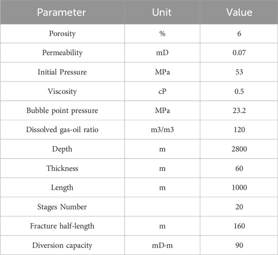
Table 1. Basic parameter of a western shale reservoir.

Table 2

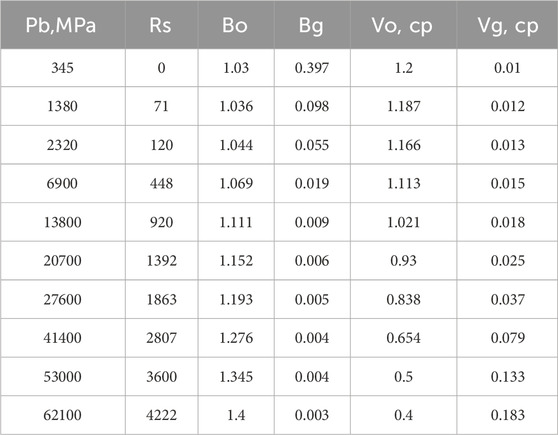
Table 2. PVT number of a western shale reservoir.

Based on the results of physical experiments, the stress sensitivity coefficient of the shale oil reservoir was fitted using an exponential form, resulting in the stress sensitivity coefficient of the shale oil reservoir (Figures 8, 9).

Figure 8

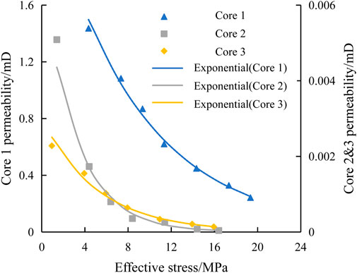
Figure 8. Measured core stress sensitivity.

Figure 9

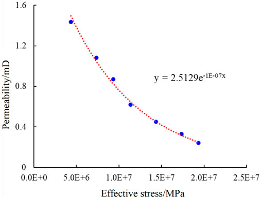
Figure 9. Stress sensitivity coefficient fitting.

Considering stress sensitivity and pressure ramp-up gradient, the complex fracture description method and fully implicit solution method proposed in this paper were utilized to study the production behavior of the shale oil reservoir. The fracture modeling method proposed in this paper accurately depicts the changes in reservoir pressure field before and after fracturing (see Figure 10).

Figure 10

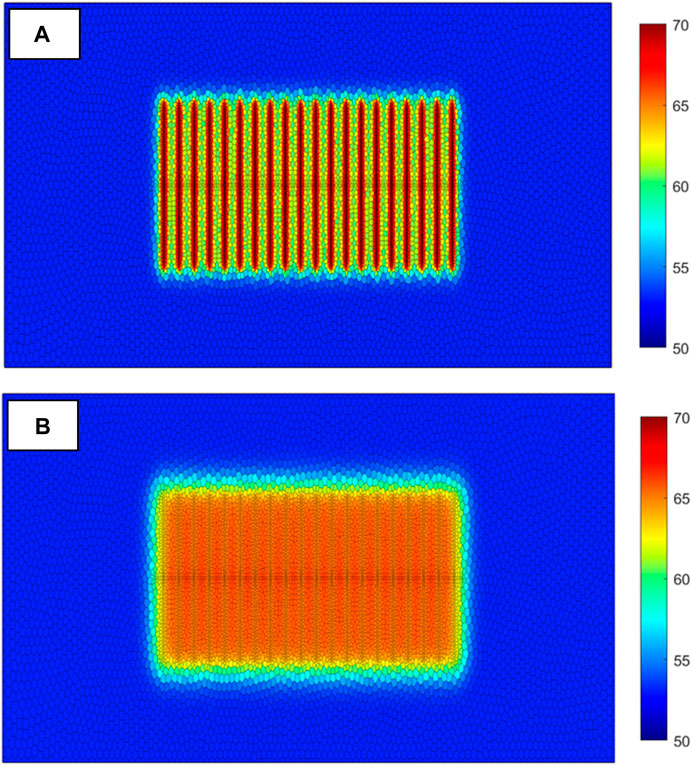
Figure 10. (A) Reservoir pressure field before fracturing and braising well (B) Reservoir pressure field after fracturing and braising well.

Simultaneously, the model validates the reservoir water saturation field and production behavior before and after fracturing. The results show that after the injection of fracturing fluid, it mainly distributes around the fractures, with relatively low water saturation between the fractures. After fracturing, the area of water saturation increase expands, and the water saturation between fractures rises, indicating that fracturing fluid can enter the matrix under the action of pressure differential and imbibition and achieve oil displacement (see Figure 11).

Figure 11

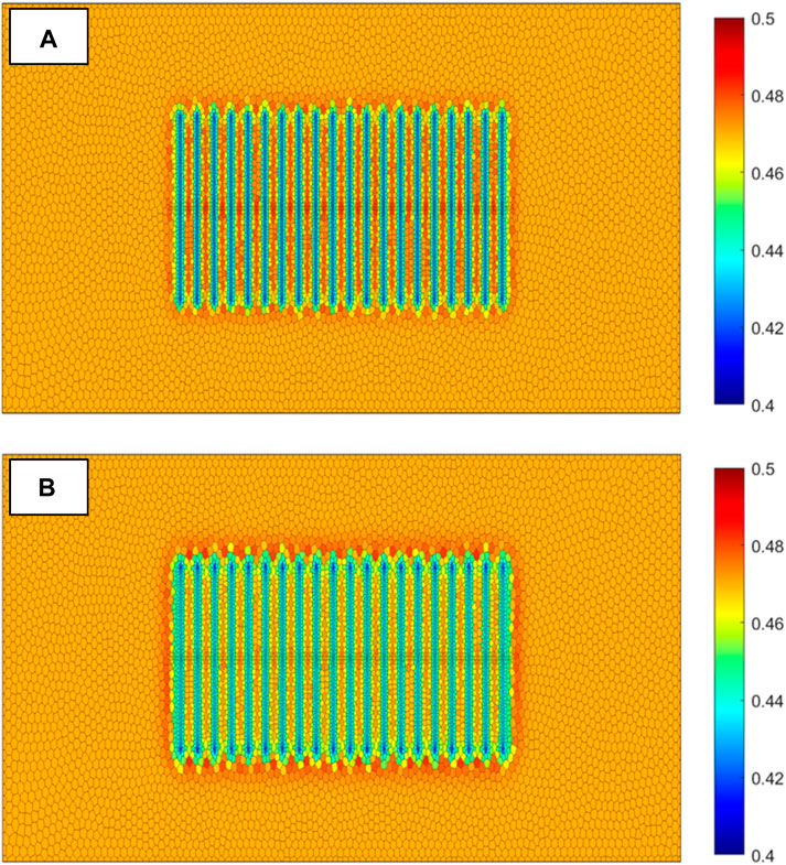
Figure 11. (A) Water saturation field before fracturing and braising well (B) Water saturation field after fracturing and braising well.

The production capacity variation curve of the shale oil reservoir block selected as an example is shown in Figure 12. Due to the backflow of fracturing fluid, the initial daily water production is the highest during the early stage of production. As the production time increases, the pressure gradually decreases, leading to a continuous decrease in water production. The oil production shows an increasing trend followed by a decreasing trend, with a maximum oil production of 92 m³/d. However, due to the gradual depletion of pressure in the reservoir modification zone at the end of the depressurization development phase, the oil production decreases rapidly after reaching its peak. In the later stage of development, the cumulative oil and water production gradually increases at a slower rate.

Figure 12

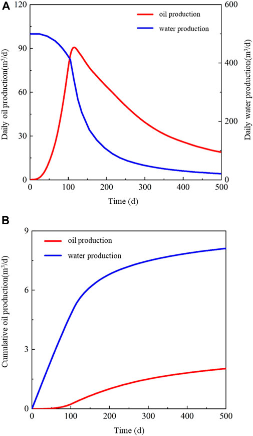
Figure 12. (A) Daily production curve (B) Cumulative yield curve.

6 Conclusion

This paper uses an embedded discrete fracture model based on a non-structural network to accurately represent complex fracture shapes and gas and water flows. The PEBI non-structured grid with good local orthogonality is used for fracture characterization. At the same time, a PEBI non-structured grid adaptive local refinement partitioning method is established, which is better adapted to the fine characterization of complex-shaped fractures in the reservoir and the reservoir grid. divide. In terms of solution, the Newton-Raphson method is used to linearize the nonlinear equation, the Jacobian matrix is ​​constructed, the ILU method is used for preprocessing, the conjugate gradient method is used for matrix solving, and a mathematical model of shale oil quasi-elastic energy development is established. Fully implicit solution method.

The example data of a shale reservoir in the west was selected for modeling and numerical verification. The complex fracture description method in this article can accurately and quickly display the changes in the reservoir field data during the numerical simulation operation. At the same time, the fully implicit solution method of the mathematical model for quasi-elastic energy development of shale oil reservoirs established in this article accurately describes production changes during the calculation process, providing strong technical support for the preparation of actual oil field development plans.

Data availability statement

The datasets presented in this article are not readily available because All data in article are not allowed to be used in any purpose. Requests to access the datasets should be directed to Jia Han, hanjia0217@petrochina.com.cn.

Author contributions

WR: Writing–original draft. LZ: Writing–review and editing. JH: Writing–review and editing.

Funding

The author(s) declare that no financial support was received for the research, authorship, and/or publication of this article. This work was supported by the National Natural Science Foundation of China (No. U22B500696).

Conflict of interest

Authors WR, LZ, JH, YYa, and YYi were employed by the company PetroChina. Author JH was employed by China Notional Petroleum Company.

Publisher’s note

All claims expressed in this article are solely those of the authors and do not necessarily represent those of their affiliated organizations, or those of the publisher, the editors and the reviewers. Any product that may be evaluated in this article, or claim that may be made by its manufacturer, is not guaranteed or endorsed by the publisher.

References

Chen, X. F., Tang, C., Du, Z. M., Tang, L. D., Wei, J. B., and Ma, X. (2018). Numerical simulation of shale gas multi-stage fracturing horizontal wells based on finite volume method. Nat. Gas. Ind. 38 (12), 77–86.

Google Scholar

Hou, B., Chang, Z., Wu, A. A., and Derek, E. (2022). Simulation of competitive propagation of multi-cluster fractures in oil-tight cutting and fracturing of shale in the Jimusar Depression. Acta Pet. Sin. 43 (1), 75–90. doi:10.7623/syxb202201007

CrossRef Full Text | Google Scholar

Meng, X. B. (2024). Numerical simulation of fracture propagation in the entire well section through staged multi-cluster fracturing of horizontal wells in shale oil reservoirs—taking the Shahejie Formation in Jiyang Depression as an example. Fault block oil gas fields, 1–12.

Google Scholar

Mirzaei, M., and Cipolla, C. L. (2012). “A workflow for modeling and simulation of hydraulic fractures in unconventional gas reservoirs,” in Paper 153022-MS presented at the SPE Middle East Unconventional Gas Conference and Exhibition, AbuDhabi, 23-25 January 2012 (AbuDhabi: UAE). doi:10.2118/153022-MS

CrossRef Full Text | Google Scholar

Wang, Y. Z., Hou, B., Wang, D., and Jia, Z. H. (2021). Characteristics of high propagation of cross-layer pressure fractures in multiple shale oil reservoirs. Petroleum Explor. Dev. 48 (2), 402–410. doi:10.11698/PED.2021.02.17

CrossRef Full Text | Google Scholar

Zhang, S. C., Li, S. H., Zou, Y. S., Li, J. M., Ma, X. F., Zhang, X. H., et al. (2021). Experiment on fracture height expansion of multi-stage fracturing in shale oil horizontal wells. J. China Univ. Petroleum Nat. Sci. Ed. 45 (1), 77–86. doi:10.3969/j.issn.1673-5005.2021.01.009

CrossRef Full Text | Google Scholar

Zhao, J. Z., Ren, L., Shen, P., and Li, Y. M. (2018). New progress in research on fracture network fracturing theory and technology of shale gas reservoirs. Nat. Gas. Ind. 38 (3), 1–14. doi:10.3787/j.issn.1000-0976.2018.03.001

CrossRef Full Text | Google Scholar

Zou, Y. S., Shi, S. Z., Zhang, S. C., Li, J. M., Wang, F., Wang, J. C., et al. (2022). Hydraulic fracture morphology and proppant distribution characteristics of thin interbedded shale oil reservoirs. Petroleum Explor. Dev. 49 (5), 1025–1032. doi:10.11698/PED.20220083

CrossRef Full Text | Google Scholar