Improved typical scenario-based distributionally robust co-dispatch of energy and reserve for renewable power systems considering the demand response of fused magnesium load

In recent years, the penetration of solar and wind power has rapidly increased to construct renewable energy-dominated power systems (RPSs). On this basis, the forecasting errors of renewable generation power have negative effects on the operation of the power system. However, traditional scheduling methods are overly dependent on the generation-side dispatchable resources and lack uncertainty modeling strategies, so they are inadequate to tackle this problem. In this case, it is necessary to enhance the flexibility of the RPS by both mining the load-side dispatchable resources and improving the decision-making model under uncertainty during the energy and reserve co-dispatch. In this paper, due to the great potential in facilitating the RPS regulation, the demand response (DR) model of fused magnesium load (FML) is first established to enable the deeper interaction between the load side and the whole RPS. Then, based on the principal component analysis and clustering algorithm, an improved typical scenario set generation method is proposed to obtain a much less conservative model of the spatiotemporally correlated uncertainty. On this basis, a two-stage distributionally robust optimization model of the energy and reserve co-dispatch is developed for the RPS considering the DR of FML. Finally, the proposed method is validated by numerical tests. The results show that the costs of day-ahead dispatch and re-dispatch are significantly decreased by using the improved typical scenario set and considering the DR of FML in regulation, which enhances the operation economy while maintaining the high reliability and safety of the RPS.

1 Introduction

Under the background of increasingly serious environmental problems and accelerated depletion of resources, renewable energy-dominated power systems (RPSs) are developing rapidly (Cai et al., 2022; Liu et al., 2023). The novelty of RPSs is reflected by two main characteristics: environmentally friendly and highly flexible. Being environmentally friendly requires the large-scale application of renewable energy sources (RESs) in generation, but the complex uncertainty of RESs poses a great challenge to power system scheduling and dispatch. Therefore, the RPS must have an abundance of dispatchable resources and effective optimal dispatch methods, which means that the RPS needs to be highly flexible (Cheng et al., 2023; Trojani et al., 2023).

In the traditional power system, dispatchable resources mainly refer to thermal power, hydropower, and other conventional units on the generation side, so the dispatch mode is generation-follow-load. However, with the progress of carbon peaking and carbon neutrality, thermal power units in the RPS will inevitably be replaced by RES generation on a large scale, causing a paradoxical situation of increasing system uncertainty and decreasing generation-side regulation capability. In this case, the demand response (DR) mechanism, as a method to exploit the potential of load-side participation in system scheduling, has gained wide attention in recent years (Xie et al., 2023; Yang et al., 2024).

Currently, most related studies focus on the DR modeling of residential loads and commercial loads (Chen et al., 2022; de Chalendar et al., 2023). Compared with residential and commercial loads, industrial loads account for a higher proportion in the whole power system. In particular, the energy-consuming industrial loads have the advantages of complete infrastructures, large capacities, and strong willingness to participate in DR, so they have huge dispatch potential. However, the relevant research studies are still insufficient at present.

As typical energy-consuming industrial loads, there have been reports about the participation of iron/steel loads and fused magnesium loads (FMLs) in DR and RPS dispatch. Boldrini et al. (2024) investigated the potential of participation in DR for the electric arc furnace (EAF) technology using hydrogen as the reductant of iron. Wang et al. (2023) considered the production plans of the steel refining process to be adjustable, so that the ladle furnaces are treated as cuttable loads and modeled as DR resources. FML was reported to participate in the primary frequency control market, and the corresponding declared capacity optimization method was proposed by Guo et al. (2023). In summary, it is the heat storage processes of the iron/steel loads and FMLs using EAFs that can be regarded as DR resources. EAFs melt raw materials with electric heating technology to manufacture products, which is simple and less sensitive to power fluctuations, making them highly flexible during RPS dispatch. In addition, EAFs typically have large capacities, so rational production arrangements for enterprises using such equipment can provide significant dispatchable capacity for the power system. Hence, it is necessary to construct DR models for these energy-consuming industrial loads, so that their flexibility can contribute to the RPS. Different from FMLs, iron/steel loads have many consecutive processes such as refining and rolling. Due to the limited amount of equipment in each process, it is necessary to consider their coordination in the DR model, which is relatively complex. Therefore, to focus on the DR potential exploitation, FMLs are taken as the representative of the energy-consuming industrial loads.

To fully utilize the flexible resources of both generation and load sides, effective dispatch decision methods are also needed to enhance the ability of the power system to cope with the uncertainty of RESs. According to decision conservativeness, commonly used methods are usually classified into two categories: scenario-based stochastic optimization (SO) and robust optimization (RO) (Mazidi et al., 2019; Tan et al., 2019; Cheng et al., 2024).

For example, a stochastic scenario-based optimization model was proposed by Derakhshandeh et al. (2017) to optimize the generation scheduling of microgrids integrated with plug-in electric vehicles. A stochastic and affinely adjustable robust optimization method was constructed by Huang et al. (2019) for the co-dispatch of energy and reserve of the RPS. However, the two methods have their drawbacks.

The SO methods rely on the uncertainty sets generated by parameterized probability distribution functions. However, it is difficult to guarantee the validity of the chosen parameterized function. In addition, the obtained uncertainty sets are less capable of considering the extreme scenarios, so the dispatch results tend to be over-optimistic and insufficiently reliable. The RO methods only consider the extreme scenarios corresponding to the uncertainty space boundaries, some of which are completely impossible in reality, so the derived dispatch schemes are overly conservative. Both methods lack the capability to deal with the spatiotemporal correlation between uncertainty variables.

To combine SO and RO to achieve complementary effects, the distributionally robust optimization (DRO) theory is proposed and gradually promoted for use, which is also convenient for taking into account the spatiotemporal correlation of uncertainty variables (Shui et al., 2019; Gao et al., 2020; Liu et al., 2022).

The balance between the economy and reliability of the decision using DRO is closely related to the way of selecting the typical scenarios of uncertainty. The space enclosed by the typical scenarios is required to contain as many samples in the historical data as possible and to contain as little redundant area where no sample is located as possible. For example, the historical samples were directly used to derive an empirical probability distribution by Wang et al. (2020), where the interval centers of the distribution were adopted as the typical scenarios to construct a DRO dispatch model for the distribution network. The Wasserstein metric-based uncertainty set construction methods are also popular choices but need to consider large numbers of historical scenarios when solving the DRO model, which causes computational burden (Saberi et al., 2021; Feizi et al., 2022; Zheng et al., 2023). In recent years, minimum volume enclosing ellipsoid (MVEE)-based uncertainty set construction methods have achieved better results in typical scenario selection. Zhang et al. (2022) first obtained the MVEE that covers all the historical samples with an iteration algorithm, and then the vertices on each symmetry axis of the MVEE are regarded as the typical scenarios. However, the space enclosed by these vertices is the inscribed polyhedron of the MVEE and is not guaranteed to cover all the historical samples. To solve this problem, an expansion method of the inscribed polyhedron was proposed by Zhang et al. (2021) to obtain the vertices of its corresponding circumscribed polyhedron. Unfortunately, although all samples are covered after such treatment, the redundant scenarios in the polyhedral space increase significantly, some of which even exceed the upper and lower bounds of the uncertainty variables. These impossible scenarios result in great conservativeness of the decision scheme, which makes the DRO lose advantages. It can be observed that directly using the vertices of the inscribed and circumscribed polyhedron as typical scenarios for DRO is inappropriate.

According to the above analysis, the RPS still has deficiencies in both flexible resource mining and dispatch capability enhancement, so this paper focuses on the relevant works shown as follows:

1) FML is taken as the representative of energy-consuming industrial loads, and its lean DR model integrated with time-coupled constraints is established to further exploit the regulation potential of the RPS load side.

2) An improved typical scenario generation method is proposed by uniting the boundary points with cluster centers of the historical samples and then adjusting the impossible points. Then, an improved typical scenario-based DRO (ITSDRO) dispatch model for the RPS is established to lower the conservativeness and achieve a better balance between reliability and economy.

The rest of the paper is organized as follows: in Section 2, the two-stage DRO model is constructed for the co-dispatch of energy and reserve for the RPS considering the DR of FML; Section 3 details the improved typical scenario set generation method, and it is integrated into the model established in Section 2; then, the solving algorithm of the proposed DRO model is given in Section 4; numerical tests are carried out and discussed in Section 5; and the conclusion is summarized in Section 6.

2 DRO co-dispatch of energy and reserve for the RPS considering the DR of FML

In this section, the two-stage DRO co-dispatch model of energy and reserve for the RPS is established considering the participation of the FML in the DR. Although only the DR of the FML is integrated into the model, DR models of other types of loads can be added conveniently.

2.1 DR model of the FML

The FML utilizes EAFs to prepare electrically fused magnesia as its product, whose main component is MgO. The production process is to use the electric arc to heat the raw materials containing MgO until they are melted in the EAF. The molten raw materials are cooled naturally, and magnesite crystals grown from the molten material are ground to obtain the magnesium sand. In this process, the EAF can lift or lower the electrode to control the current, so it can regulate its power consumption. Since the rated power of a single EAF can reach the MW class, the participation of the FML in the DR project provides considerable flexible capacity for the RPS dispatch.

However, as one type of high energy-consuming industrial load, the pre-requisite for the participation of the FML in the DR is to ensure its production safety and the achievability of production tasks. Hence, it is necessary to construct the DR model of a single EAF based on the constraints in the production process and then to form the DR model of the FML accordingly.

2.1.1 Regulation capacity constraints of the EAF

$P_{m,t}^{\mathrm{M}}=P_{m,t}^{\mathrm{M},\text{base}}+P_{m,t}^{\mathrm{M},\mathrm{u}}-P_{m,t}^{\mathrm{M},\mathrm{d}},(1)$

$.0\le P_{m,t}^{\mathrm{M},\mathrm{u}}\le s_{m,t}^{\mathrm{u}}{P}_{\max ,m}^{\mathrm{u}},0\le P_{m,t}^{\mathrm{M},\mathrm{d}}\le s_{m,t}^{\mathrm{d}}{P}_{\max ,m}^{\mathrm{d}},(2)$

$s_{m,t}^{\mathrm{u}}+s_{m,t}^{\mathrm{d}}=1,(3)$

where t is the index of time. $P_{m,t}^M$ is the regulated power of the mth EAF. $P_{m,t}^{\mathrm{M},\text{base}}$ is the base power of the mth EAF. $P_{m,t}^{\mathrm{M},\mathrm{u}}$ and $P_{m,t}^{\mathrm{M},\mathrm{d}}$ are the upward and downward regulated power of the mth EAF, respectively; $P_{\max ,m}^{\mathrm{u}}$ and $P_{\max ,m}^{\mathrm{d}}$ are the upper limits of $P_{m,t}^{\mathrm{M},\mathrm{u}}$ and $P_{m,t}^{\mathrm{M},\mathrm{d}}$ due to the safety consideration, respectively; and $s_{m,t}^{\mathrm{u}}$ and $s_{m,t}^{\mathrm{d}}$ are binary variables indicating the EAF to be in upward and downward regulation states, respectively.

2.1.2 Constraints of regulation times of the EAF

Within a day, the total upward and downward regulation times of an EAF should not exceed a scheduled maximum number. This avoids the overly frequent regulation of one EAF and ensures its productivity and product purity.

$0\le {\displaystyle \sum _{t=2}^T}\left|s_{m,t}^{\mathrm{u}}-s_{m,t-1}^{\mathrm{u}}\right|\le M,(4)$

where M is the scheduled maximum regulation number of one EAF in 1 day. T is the number of time slots in 1 day.

Upward and downward regulation times are both considered in (4), which is intuitively demonstrated by introducing binary auxiliary variables in Section 2.2.4.

2.1.3 Regulation duration constraints of the EAF

One EAF should not be in the upward regulation state for several consecutive periods; otherwise, the temperature of the molten liquid continues to increase, resulting in accidents such as furnace eruption. In addition, if the power of the EAF is continuously regulated downward for too long, the temperature in the furnace cannot meet the production requirements, which affects the purity of the products. Therefore, the upward and downward regulation duration constraints of the EAF are constructed as follows:

$\left\{\begin{array}{l}{s}_{m,t}^{\mathrm{u}}\left(T_m^{\mathrm{u}}-{\displaystyle \sum _{\tau =t-T_m^{\mathrm{u}}-1}^{t-1}}{s}_{m,\tau }^{\mathrm{u}}\right)\ge 0\\ s_{m,t}^{\mathrm{d}}\left(T_m^{\mathrm{d}}-{\displaystyle \sum _{\tau =t-T_m^{\mathrm{d}}-1}^{t-1}}{s}_{m,\tau }^{\mathrm{d}}\right)\ge 0\end{array}\right.,(5)$

where $T_m^{\mathrm{u}}$ and $T_m^{\mathrm{d}}$ are the maximum duration of upward and downward power regulation of the EAF, respectively.

2.1.4 Constraints of the power and production of the FML

The power consumed by the FML is accumulated from all EAFs:

${\displaystyle \sum _m}{P}_{m,t}^{\mathrm{M}}=P_t^{\text{FML}},(6)$

where $P_{\text{FML}}\left(t\right)$ is the total power of all the EAFs belonging to the FML at time t.

Then, the FML is modeled as a shiftable load in (7), which means that the energy consumed in 1 day should remain unchanged whether FML participates in DR projects or not. This constraint ensures that production is not affected by the DR.

${\displaystyle \sum _t}{\displaystyle \sum _m}{P}_{m,t}^{\mathrm{M},\text{base}}={\displaystyle \sum _t}{P}_t^{\text{FML}}.(7)$

2.2 Construction of the two-stage DRO co-dispatch model

To optimize the day-ahead energy and reserve strategy of the RPS, the DRO model constructed in this paper is composed of two stages. In the first stage, the base case of the day-ahead RES and load prediction is used to optimize the unit commitment and reserved capacity of conventional units. In the second stage, a prediction error scenario set is constructed and used to optimize the operation of flexible resources to ensure the RPS reliability considering the day-ahead RES and load prediction uncertainty.

By the interaction of decision variables of the two stages, the determined unit commitment and reserved capacity finally achieve a balance between reliability and economy.

2.2.1 Objective function

The overall objective of the proposed model is to minimize the total operation costs of the two stages, as shown in (8):

$\underset{x}{\min }{C}_{\text{op}}\left(\mathit{x}\right)+\underset{p_k\in \mathrm{\Omega }}{\max }{\displaystyle \sum _{k=1}^{n_{\text{sce}}}}{p}_k\underset{y_k}{\min }{C}_{\text{reg}}\left(\mathit{x},{\mathit{y}}_k\right),(8)$

$\begin{array}{c}\mathit{x}=\left[I_{i,t},P_{i,t},{\alpha }_{i,t}^{\mathrm{u}},{\alpha }_{i,t}^{\mathrm{d}},R_{i,t}^{\mathrm{u}},R_{i,t}^{\mathrm{d}}\right]\\ {\mathit{y}}_k=\left[P_{i,t,k}^{\mathrm{u}},P_{i,t,k}^{\mathrm{d}},W_{w,t,k}^{\text{cur}},L_{b,t,k}^{\text{sh}},P_{m,t,k}^{\mathrm{M},\mathrm{u}},P_{m,t,k}^{\mathrm{M},\mathrm{d}},s_{m,t,k}^{\mathrm{u}},s_{m,t,k}^{\mathrm{d}}\right]\end{array},(9)$

where x and C_op(x) are the decision variables and objective function in the first stage, respectively. The values of x remain unchanged during the optimization of the second stage. n_sce is the number of prediction error scenarios employed in the second stage. k is the index of the scenarios. p_k is the occurrence of scenario k. Ω is the uncertainty space of the probability distribution {p_k|k = 1, … ,n_sce}. y_k and C_reg(x, y_k) are the decision variables and objective function in the second stage, respectively.

According to (8), the two-stage dispatch model is established based on the DRO theory. The max–min structure in the second stage is used to search for the worst distribution of the prediction error scenarios within Ω, which ensures that the optimized strategy can adapt to this worst distribution, so that the reliability and economy are balanced.

The functions of C_op(x) and C_reg(x, y_k) are shown as (10) and (11), respectively:

$C_{\text{op}}\left(x\right)={\displaystyle \sum _t}\left[{\displaystyle \sum _i}{C}_i^{\text{fuel}}{F}_i\left(P_{i,t}\right)+{\displaystyle \sum _i}\left(S_i^{\mathrm{u}}{\alpha }_{i,t}^{\mathrm{u}}+S_i^{\mathrm{d}}{\alpha }_{i,t}^{\mathrm{d}}\right)+{\displaystyle \sum _i}\left(C_i^{\mathrm{u}}{R}_{i,t}^{\mathrm{u}}+C_i^{\mathrm{d}}{R}_{i,t}^{\mathrm{d}}\right)\right],(10)$

$C_{\text{reg}}\left(x,y_k\right)={\displaystyle \sum _t}\left[{\displaystyle \sum _i}\left(Q_i^{\mathrm{u}}{P}_{i,t,k}^{\mathrm{u}}+Q_i^{\mathrm{d}}{P}_{i,t,k}^{\mathrm{d}}\right)+{\displaystyle \sum _w}{C}^{\mathrm{w}}{W}_{w,t,k}^{\text{cur}}+{\displaystyle \sum _b}{C}^{\text{ld}}{L}_{b,t,k}^{\text{cur}}|+|{\displaystyle \sum _m}\left(C^{\mathrm{M},\mathrm{u}}{s}_{m,t,k}^{\mathrm{u}}+C^{\mathrm{M},\mathrm{d}}{s}_{m,t,k}^{\mathrm{d}}\right)\right],(11)$

where $C_i^{\text{fuel}}$ is the fuel price of unit i. $F_i\left(\cdot \right)$ is the linearized function of the consumed fuel and the power output of unit i. $R_{i,t}^{\mathrm{u}}$ and $R_{i,t}^{\mathrm{d}}$ are upward and downward reserve capacity of unit i at time t, respectively. $S_i^{\mathrm{u}}$ and $S_i^{\mathrm{d}}$ are startup and shutdown costs of unit i, respectively. ${\alpha }_{i,t}^{\mathrm{u}}$ and ${\alpha }_{i,t}^{\mathrm{d}}$ are binary variables of unit i indicating the occurrence of startup and shutdown at time t, respectively. $C_i^{\mathrm{u}}$ and $C_i^{\mathrm{d}}$ are the up and down reserve prices of unit i, respectively. $P_{i,t,k}^{\mathrm{u}}$ and $P_{i,t,k}^{\mathrm{d}}$ are the upward and downward regulated powers of unit i at time t in scenario k, respectively. $Q_i^{\mathrm{u}}$ and $Q_i^{\mathrm{d}}$ are up and downregulation prices of unit i, respectively. $W_{w,t,k}^{\text{cur}}$ and $L_{b,t,k}^{\text{cur}}$ are the amount of curtailed power of RES station w and load shedding of bus b at time t in scenario k, respectively. $C^{\mathrm{w}}$ and $C^{\text{ld}}$ are the penalty prices of RES curtailment and load shedding, respectively. C^M,u and C^M,d are the subsidized prices of upward and downward regulation of the FML, respectively.

2.2.2 Power system operation constraints

The constraints in the first stage correspond to the RES power prediction base case. The constraints in the second stage correspond to the RES power prediction error cases. The details are given below.

Constraints in the first stage:

(1) Minimum up/down time of conventional units:

$\left\{\begin{array}{l}\left({\displaystyle \sum _{\tau =t-T_i^{\text{on}}}^{t-1}}{I}_{i,\tau }-T_i^{\text{on}}\right)\left(I_{i,t-1}-I_{i,t}\right)\ge 0\\ \left({\displaystyle \sum _{\tau =t-T_i^{\text{off}}}^{t-1}}\left(1-I_{i,\tau }\right)-T_i^{\text{off}}\right)\left(I_{i,t}-I_{i,t-1}\right)\ge 0\end{array}\right.,(12)$

where $T_i^{\text{on}}$ and $T_i^{\text{off}}$ are the minimum duration of the on and off statuses of unit i, respectively. $I_{i,t}$ is a binary variable of unit i at time t, which takes 1 for the on status and 0 for the off status.

(2) Startup and shutdown limits of conventional units:

$\left\{\begin{array}{l}{\alpha }_{i,t}^{\mathrm{u}}-{\alpha }_{i,t}^{\mathrm{d}}=I_{i,t}-I_{i,t-1}\\ {\alpha }_{i,t}^{\mathrm{u}}+{\alpha }_{i,t}^{\mathrm{d}}\le 1\end{array}\right..(13)$

(3) Output power and ramp rate limits of conventional units:

$\left\{\begin{array}{l}{I}_{i,t}{P}_{i,\min }\le P_{i,t}\le I_{i,t}{P}_{i,\max }\\ -D{R}_i\le P_{i,t}-P_{i,t-1}\le U{R}_i\end{array}\right.,(14)$

where P_i,min and P_i,max are the minimum and maximum output power of unit i, respectively. UR_i and DR_i are the maximum upward and downward ramp power of unit i, respectively.

(4) Limits of the unit reserve capacity and system reserve requirement:

$\left\{\begin{array}{l}0\le R_{i,t}^{\mathrm{u}}\le \min \left(U{R}_i,I_{i,t}{P}_{i,\max }-P_{i,t}\right)\\ 0\le R_{i,t}^{\mathrm{d}}\le \min \left(D{R}_i,P_{i,t}-I_{i,t}{P}_{i,\min }\right)\end{array}\right.,(15)$

${\displaystyle \sum _i}{R}_{i,t}^{\mathrm{u}}\ge R_t^{\mathrm{u}},{\displaystyle \sum _i}{R}_{i,t}^{\mathrm{d}}\ge R_t^{\mathrm{d}},(16)$

where $R_t^{\mathrm{u}}$ and $R_t^{\mathrm{d}}$ are the upward and downward reserve power requirements of the RPS at time t, respectively.

(5) Power balance limits:

${\displaystyle \sum _i}{P}_{i,t}+{\displaystyle \sum _w}{\widehat{W}}_{w,t}={\displaystyle \sum _b}{L}_{b,t}+{\displaystyle \sum _m}{P}_{m,t}^{\mathrm{M},\text{base}},(17)$

where ${\widehat{W}}_{w,t}$ is the predicted output power of RES station w at time t in the base case. ${\widehat{L}}_{b,t}$ is the predicted load consumption of bus b at time t in the base case.

(6) Transmission capacity limits of power lines based on the DC power flow model:

$\left|{\displaystyle \sum _b}{k}_{lb}({\displaystyle \sum _{i\in b}}{P}_{i,t}+{\displaystyle \sum _{w\in b}}{\widehat{W}}_{w,t}-{\widehat{L}}_{b,t}-{\displaystyle \sum _{m\in b}}{P}_{m,t}^{\mathrm{M},\text{base}}\right|\le f_{l\max },(18)$

where k_lb is the power transfer distribution factor of bus b to line l, which represents the DC power flow model (Cai and Xu, 2021). f_lmax is the maximum transmission power of line l.

Constraints in the second stage:

(1) Output power and ramp rate limits of conventional units:

$\left\{\begin{array}{l}{I}_{i,t}{P}_{i,\min }\le P_{i,t}+P_{i,t,k}^{\mathrm{u}}-P_{i,t,k}^{\mathrm{d}}\le I_{i,t}{P}_{i,\max }\\ -D{R}_i\le P_{i,t}+P_{i,t,k}^{\mathrm{u}}-P_{i,t,k}^{\mathrm{d}}-\left(P_{i,t-1}+P_{i,t-1,k}^{\mathrm{u}}-P_{i,t-1,k}^{\mathrm{d}}\right)\le U{R}_i.\\ 0\le P_{i,t,k}^{\mathrm{u}}\le R_{i,t}^{\mathrm{u}}\\ 0\le P_{i,t,k}^{\mathrm{d}}\le R_{i,t}^{\mathrm{d}}\end{array}\right.(19)$

(2) Power balance limits:

${\displaystyle \sum _i}\left(P_{i,t}+P_{i,t,k}^{\mathrm{u}}-P_{i,t,k}^{\mathrm{d}}\right)+{\displaystyle \sum _w}\left({\widehat{W}}_{w,t}+\Delta W_{w,t,k}-W_{w,t,k}^{\text{cur}}\right)={\displaystyle \sum _b}\left({\widehat{L}}_{b,t}+\Delta L_{b,t,k}-L_{b,t,k}^{\text{sh}}\right)+{\displaystyle \sum _m}{P}_{m,t}^{\mathrm{M}},(20)$

where ΔW_w,t,k and ΔL_b,t,k are the prediction error of RES station w and bus b at time t in scenario k, respectively.

(3) Transmission capacity limits of power lines based on the DC power flow model:

$\begin{array}{l}\left|{\displaystyle \sum _b}{k}_{lb}\left[{\displaystyle \sum _{i\in b}}\left(P_{i,t}+P_{i,t,k}^{\mathrm{u}}-P_{i,t,k}^{\mathrm{d}}\right)+{\displaystyle \sum _{w\in b}}\left({\widehat{W}}_{w,t}+\Delta W_{w,t,k}-W_{w,t,k}^{\text{cur}}\right)\right.\right.\\ \left.\left.-\left({\widehat{L}}_{b,t}+\Delta L_{b,t,k}-L_{b,t,k}^{\text{sh}}\right)-{\displaystyle \sum _{m\in b}}{P}_{m,t}^{\mathrm{M}}\right]\right|\le f_{l\max }\end{array}.(21)$

(4) Wind curtailment and load shedding limits:

$\left\{\begin{array}{l}0\le W_{w,t,k}^{\text{cur}}\le {\widehat{W}}_{w,t}+\Delta W_{w,t,k}\\ 0\le L_{b,t,k}^{\text{sh}}\le {\widehat{L}}_{b,t}+\Delta L_{b,t,k}\end{array}\right..(22)$

(5) FML constraints

As indicated by (9), the DR of the FML is regarded as a flexible resource to cope with the prediction errors of the RES output. Therefore, (1–7) are treated as constraints in the second stage, where the FML decision variables should be included in y_k and the index k needs to be added to these variables.

2.2.3 Power prediction error probability distribution constraints

Using the norm-1 and norm-inf, the uncertainty space Ω in (8) can be constructed by the power prediction error probability distribution constraints below:

$\mathrm{\Omega }=\left\{p_k:\begin{array}{l}{\displaystyle \sum _{k=1}^{N_{\text{sce}}}}{p}_k=1,p_k\ge 0\\ {\displaystyle \sum _{k=1}^{N_{\text{sce}}}}\left|p_k-p_{k0}\right|\le {\theta }_1\\ \underset{1\le k\le N_{\text{sce}}}{\max }\left|p_k-p_{k0}\right|\le {\theta }_{\infty }\end{array}\right\},(23)$

where p_k0 is the initial probability of scenario k obtained by analyzing the historical samples. θ₁ and θ_∞ are the variation tolerance in the form of norm-1 and norm-inf, respectively, which can be calculated with the formula given by Wang et al. (2020).

The non-linear absolute term in (23) is linearized by introducing auxiliary variables. The constraints of these auxiliary variables are given below:

$\left\{\begin{array}{l}{z}_{k+}+z_{k-}\le 1\\ 0\le p_{k+}\le z_{k+}{\theta }_1,\hspace{1em}0\le p_{k-}\le z_{k-}{\theta }_1\\ 0\le p_{k+}\le z_{k+}{\theta }_{\infty },\hspace{1em}0\le p_{k-}\le z_{k-}{\theta }_{\infty }\end{array}\right.,(24)$

where z_k+ and z_k− are binary auxiliary variables. p_k+ and p_k− are real auxiliary variables.

The linearized form of (23) is shown as

$\left\{\begin{array}{l}{p}_k=p_{k0}+p_{k+}-p_{k-}\\ {\displaystyle \sum _{k=1}^{N_{\text{sce}}}}\left(p_{k+}+p_{k-}\right)\le {\theta }_1\\ p_{k+}+p_{k-}\le {\theta }_{\infty }\end{array}\right..(25)$

2.2.4 Linearization of non-convex constraints

The constraints shown in (4), (5), (12), and (15) are non-convex, so the formulated model above cannot be directly solved by common commercial solvers. In this section, they are all linearized to obtain an equivalent convex form of the proposed DRO model.

For (4), binary auxiliary variables are introduced to derive its equivalent linearized form as shown below:

$\left\{\begin{array}{l}{z}_{m,t}^{\mathrm{u}}+z_{m,t}^{\mathrm{d}}\le 1\\ s_{m,t}^{\mathrm{u}}-s_{m,t-1}^{\mathrm{u}}=z_{m,t}^{\mathrm{u}}-z_{m,t}^{\mathrm{d}}\\ 0\le {\displaystyle \sum _{t=2}^T}\left(z_{m,t}^{\mathrm{u}}+z_{m,t}^{\mathrm{d}}\right)\le M\end{array}\right.,(26)$

where $z_{m,t}^{\mathrm{u}}$ and $z_{m,t}^{\mathrm{d}}$ are the introduced pair of binary variables. $z_{m,t}^{\mathrm{u}}$ = 1 indicates that upward regulation happens in time t. Similarly, $z_{m,t}^{\mathrm{d}}$ is the indicator of downward regulation.

For (5) and (12), both are the constraints of duration, so they have nearly the same structure. For such a structure, the linearized form is obtained by dividing T into three sections, which is given by Carrion and Arroyo (2006). For succinctness, the deduction is not repeated here.

For (15), the non-convexity of the two constraints is aroused by the nested min terms. Each of them can be replaced by two separated constraints to avoid the usage of the min terms, which is shown below:

$\left\{\begin{array}{l}0\le R_{i,t}^{\mathrm{u}}\le U{R}_i,\hspace{1em}{R}_{i,t}^{\mathrm{u}}\le I_{i,t}{P}_{i,\max }-P_{i,t}\\ 0\le R_{i,t}^{\mathrm{d}}\le D{R}_i,\hspace{1em}{R}_{i,t}^{\mathrm{d}}\le P_{i,t}-I_{i,t}{P}_{i,\min }\end{array}\right..(27)$

3 Improved typical scenario set generation method

Whether the balance between economy and reliability can be achieved or not by DRO is closely related to the way how typical scenarios of prediction errors are selected. Previous DRO methods usually adopt the cluster centers of historical prediction errors as the typical scenarios, which are unable to test whether the determined day-ahead strategy can cope with the possible extreme prediction errors or not. Hence, these methods are too optimistic to consider the uncertainty in the day-ahead stage thoroughly. However, if the traditional box uncertainty set of RO is directly transferred to DRO, the spatiotemporal correlation between RES power outputs and loads is neglected, which results in an overconservative decision. In this case, to consider the spatiotemporal correlation, an MVEE containing all the historical prediction error samples is often constructed. The vertices of its inscribed and circumscribed polyhedra are used as the typical scenarios, which is shown by Figure 1 (Zhang et al., 2021; Zhang et al., 2022).

Figure 1

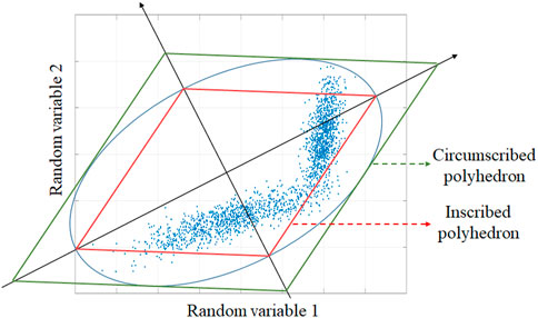
Figure 1. Typical scenario sets constructed by the circumscribed and inscribed polyhedra of the MVEE.

As shown in Figure 1, the inscribed polyhedron is unable to cover all the historical samples. In addition, for both the inscribed and circumscribed polyhedra, the coordinate values of the vertices may exceed the maximum or minimum values of the historical samples.

To solve this dilemma, an improved typical scenario set generation method is proposed based on the principal component analysis and K-means clustering algorithm, which unites the cluster centers and the extreme points of the historical prediction error samples to reduce decision conservativeness while maintaining reliability.

1) The prediction error vector is denoted by Eq. 28

$\mathit{u}=\left[\Delta \mathit{W},\Delta \mathit{L}\right],(28)$

where ΔW and ΔL are the power prediction error vector of RES stations and load buses, respectively, which are detailed by Eq. 29

$\begin{array}{l}\Delta \mathit{W}=\left[\Delta W_{1,1},...,\Delta W_{w,t},...,\Delta W_{N_{\mathrm{W}},T}\right]\\ \Delta \mathit{L}=\left[\Delta L_{1,1},...,\Delta L_{b,t},...,\Delta L_{N_{\mathrm{b}},T}\right]\end{array},(29)$

where N_W is the total number of RES stations. N_b is the total number of load buses.

2) The eigenvectors are computed, and the coordinates of the vertices along the direction of each eigenvector are obtained. Zhang et al. (2022); Zhang et al. (2021) used the iterative MVEE algorithm to obtain these coordinates, but the iteration will significantly decelerate when the area covered by historical samples lacks symmetry. Therefore, the iteration-free principal component analysis algorithm is chosen to obtain the abovementioned eigenvectors and vertices quickly and accurately. The process is detailed below.

The historical prediction error samples of the RES stations and load buses are denoted as matrix U in Eq. 30

$\mathit{U}={\left[{\mathit{u}}_1,...,{\mathit{u}}_s,...,{\mathit{u}}_N\right]}^T.(30)$

U is processed with the zero mean method as shown in Eq. 30:

$\stackrel{\sim }{\mathit{U}}=\mathit{U}-1_N\otimes {\overline{\mathit{u}}}^T={\left[{\stackrel{\sim }{\mathit{u}}}_1,...,{\stackrel{\sim }{\mathit{u}}}_s,...,{\stackrel{\sim }{\mathit{u}}}_N\right]}^T,(31)$

where $\stackrel{\sim }{\mathit{U}}$ is the version of U after the zero mean processing. $\overline{\mathit{u}}$ is the mean vector of all historical samples. ${\stackrel{\sim }{\mathit{u}}}_s$ is the sth sample after the zero mean processing. N is the number of historical samples.

The covariance matrix of $\stackrel{\sim }{\mathit{U}}$ is obtained, and then, eigenvalue decomposition on the covariance matrix is performed by Eq. 32:

$\left\{\begin{array}{l}\mathit{S}=\frac{1}{N-1}{\stackrel{\sim }{\mathit{U}}}^T\stackrel{\sim }{\mathit{U}}\\ \mathit{S}=\mathit{Q}\mathit{\Lambda }{\mathit{Q}}^T\\ \mathit{Q}=\left[{\mathit{q}}_1,....,{\mathit{q}}_h,....,{\mathit{q}}_{\left(N_{\mathrm{b}}+N_{\mathrm{W}}\right)T}\right]\\ \mathit{\Lambda }=diag\left\{{\lambda }_1,...,{\lambda }_h,...,{\lambda }_{\left(N_{\mathrm{b}}+N_{\mathrm{W}}\right)T}\right\}\end{array}\right.,(32)$

where S is the covariance matrix of $\stackrel{\sim }{\mathit{U}}$. q_h is the hth eigenvector of S. λ_h is the eigenvalue corresponding to q_h. Λ is a diagonal matrix formed by all eigenvalues.

Each sample in $\stackrel{\sim }{\mathit{U}}$ is transformed into a new coordinate system defined by the eigenvectors as shown in Eq. 33

${\stackrel{\sim }{\mathit{v}}}_s={\mathit{Q}}^T{\stackrel{\sim }{\mathit{u}}}_s={\left[{\stackrel{\sim }{v}}_{1,s},\cdots ,{\stackrel{\sim }{v}}_{h,s},\cdots ,{\stackrel{\sim }{v}}_{\left(N_{\mathrm{b}}+N_{\mathrm{W}}\right)T,s}\right]}^T,(33)$

where ${\stackrel{\sim }{\mathit{v}}}_s$ is the projection point of ${\stackrel{\sim }{\mathit{u}}}_s$ in the eigenvector coordinate system. ${\stackrel{\sim }{v}}_{h,s}$ is the projection value of ${\stackrel{\sim }{\mathit{u}}}_s$ in the direction of q_h.

After all samples are projected, the coordinates of the two vertices are determined in the direction of each eigenvector by Eq. 34

$\left\{\begin{array}{l}{\stackrel{\sim }{\mathit{v}}}_h^{\min }=\min \left\{{\stackrel{\sim }{v}}_{h,1},\cdots ,{\stackrel{\sim }{v}}_{h,N}\right\}\cdot {\mathit{e}}_h\\ {\stackrel{\sim }{\mathit{v}}}_h^{\max }=\max \left\{{\stackrel{\sim }{v}}_{h,1},\cdots ,{\stackrel{\sim }{v}}_{h,N}\right\}\cdot {\mathit{e}}_h\end{array}\right.,(34)$

where ${\stackrel{\sim }{\mathit{v}}}_h^{\min }$ and ${\stackrel{\sim }{\mathit{v}}}_h^{\max }$ are the coordinates of the two vertices in the direction of the hth eigenvector under the eigenvector coordinate system. e_h is a unit vector, with the hth element equal to 1.

3) All the vertices obtained above enclose the inscribed polyhedron. Then, the scaling factor η is introduced by Eqs 35 and 36 to expand it to the circumscribed polyhedron.

$\begin{array}{l}\min {\displaystyle \sum _{s=1}^N}{‖{\mathit{\beta }}_s‖}_1\\ \mathrm{s}.\mathrm{t}.\left\{\begin{array}{l}\left[{\stackrel{\sim }{\mathit{v}}}_1^{\min },\cdots ,{\stackrel{\sim }{\mathit{v}}}_{\left(N_{\mathrm{b}}+N_{\mathrm{W}}\right)T}^{\max }\right]\left[{\mathit{\beta }}_1,...,{\mathit{\beta }}_s,...,{\mathit{\beta }}_N\right]=\left[{\stackrel{\sim }{\mathit{v}}}_1,...,{\stackrel{\sim }{\mathit{v}}}_s,...,{\stackrel{\sim }{\mathit{v}}}_N\right]\\ {\mathit{\beta }}_s={\left[{\beta }_{1,s},\cdots ,{\beta }_{2\left(N_{\mathrm{W}}+N_{\mathrm{b}}\right)T,s}\right]}^T\end{array}\right.\end{array},(35)$

$\eta =\max \left\{{‖{\mathit{\beta }}_1‖}_1,\cdots ,{‖{\mathit{\beta }}_N‖}_1\right\},(36)$

where ||β_s||₁ is the norm-1 of β_s.

The vertices of the circumscribed polyhedron under the original coordinate system are calculated as

$\left\{\begin{array}{l}{\mathit{u}}_h^{\min }=\eta \mathit{Q}{\stackrel{\sim }{\mathit{v}}}_h^{\min }+\overline{\mathit{u}}\\ {\mathit{u}}_h^{\max }=\eta \mathit{Q}{\stackrel{\sim }{\mathit{v}}}_h^{\max }+\overline{\mathit{u}}\end{array}\right.,(37)$

where ${\mathit{u}}_h^{\min }$ and ${\mathit{u}}_h^{\max }$ are the coordinates of two vertices in the direction of q_h under the original coordinate system.

As shown in Figure 1, some coordinate values of the vertices obtained by (37) may exceed the limits of the historical samples, which is impossible in the actual operation. Hence, adjustment is designed and imposed on these vertices by Eq. 38

$u_{h,e}^{\min \text{or}\max }=\left\{\begin{array}{l}\max \left\{u_{1,e},\cdots ,u_{N,e}\right\}{u}_{h,e}^{\min \text{or}\max }>\max \left\{u_{1,e},\cdots ,u_{N,e}\right\}\\ \min \left\{u_{1,e},\cdots ,u_{N,e}\right\}{u}_{h,e}^{\min \text{or}\max }<\min \left\{u_{1,e},\cdots ,u_{N,e}\right\}\\ u_{h,e}^{\min \text{or}\max }\text{\hspace{0.5em}otherwise}\end{array}\right.,(38)$

where $u_{h,e}^{\min \text{or}\max }$ represents the eth element of ${\mathit{u}}_h^{\min }$ or ${\mathit{u}}_h^{\max }$.

The adjusted vertices of the circumscribed polyhedron are the extreme scenarios of the prediction errors. They are denoted as u^vtx, which contains 2(N_b + N_w)T scenarios and shown in Eq. 39

$\begin{array}{l}{\mathit{u}}^{\text{vtx}}=\left\{{\mathit{u}}_h^{\min },{\mathit{u}}_h^{\max }|h=1,\cdots ,\left(N_{\mathrm{b}}+N_{\mathrm{W}}\right)T\right\}\\ =\left\{{\mathit{u}}_j^{\text{vtx}}|j=1,\cdots ,2\left(N_{\mathrm{b}}+N_{\mathrm{W}}\right)T\right\}\end{array}.(39)$

4) The attribution of each historical sample to every extreme scenario is analyzed.

First, the Euclidean distance between each extreme scenario in u^vtx and every historical sample is computed by Eq. 40.

$d_{s,j}={‖{\mathit{u}}_s-{\mathit{u}}_j^{\text{vtx}}‖}_2,(40)$

where d_s,j is the Euclidean distance between the sth sample u_s and the jth extreme scenario ${\mathit{u}}_j^{\text{vtx}}$.

Then, u_s is attributed to the nearest extreme scenario by Eq. 41.

$\left\{\begin{array}{l}j=\arg \underset{j}{\min }{d}_{s,j}\\ n\left(j\right)=n\left(j\right)+1\end{array}\right.,(41)$

where the array n is a 2(N_b + N_w)-dimensional vector with all its components initialized to 0.

Every time a sample is attributed to the jth extreme scenario, the kth element of array n is incremented by 1. After this operation is performed for each sample, the final n is the one that reflects the attribution of samples to extreme scenarios.

5) The K-means algorithm is used to obtain the cluster centers of historical samples, which is denoted by u^clu. At the same time, the proportion of each cluster is derived and regarded as the occurrence of the corresponding cluster center, which is shown in Eq. 42.

$\begin{array}{l}{\mathit{u}}^{\text{clu}}=\left\{{\mathit{u}}_1^{\text{clu}},\cdots ,{\mathit{u}}_o^{\text{clu}},\cdots ,{\mathit{u}}_{n_{\text{clu}}}^{\text{clu}}\right\}\\ {\mathit{p}}^{\text{clu}}=\left\{p_1^{\text{clu}},\cdots ,p_o^{\text{clu}},\cdots ,p_{n_{\text{clu}}}^{\text{clu}}\right\}\end{array},(42)$

where ${\mathit{u}}_o^{\text{clu}}$ is the oth cluster center. $p_o^{\text{clu}}$ is the occurrence of the oth cluster center. n_clu is the number of cluster centers, which can be adaptively determined by the contour coefficient, Calinski–Harabasz criterion, and so on (Balavand et al., 2018; Yuan and Yang, 2019; Karna and Gibert, 2022).

6) u^clu and u^vtx are incorporated to form the improved typical scenario set u^typ by Eq. 43, whose scenario number is the value of n_sce in (8).

${\mathit{u}}^{\text{typ}}=\left\{{\mathit{u}}^{\text{vtx}},{\mathit{u}}^{\text{clu}}\right\}=\left\{{\mathit{u}}_k^{\text{typ}}|k=1,\cdots ,n_{\text{sce}}\right\}.(43)$

Subsequently, the initial probability of each typical scenario in u^typ is determined by (44).

$p_{k0}=\left\{\begin{array}{l}\frac{n\left(j\right)}{N}\cdot \omega ,\hspace{1em}if{\mathit{u}}_k^{\text{typ}}={\mathit{u}}_j^{\text{vtx}}\\ p_o^{\text{clu}}\cdot \left(1-\omega \right),\hspace{1em}if{\mathit{u}}_k^{\text{typ}}={\mathit{u}}_o^{\text{clu}}\end{array}\right.,(44)$

where p_k0 is the initial probability of ${\mathit{u}}_k^{\text{typ}}$. ω is the weight of extreme scenarios in the typical scenario set, which is determined by the system operators according to the actual RPS structure and expected reliability level.

Apparently, the improved typical scenario set u^typ includes both adjusted extreme scenarios and cluster centers, so the conservativeness is reduced.

4 Solution method

Combining Sections 2 and 3, the ITSDRO model for the co-dispatch of energy and reserve is finally established for the RPS. The objective function is composed of (8), (10)–(11), and the constraints are shown as (1)–(7), (12)–(22), and (24)–(27). For a given first-stage decision variable x, if there exists a second-stage decision variable y that can ensure the steady operation of the RPS under all extreme scenarios, then x is a robust solution to the RPS dispatch problem.

The proposed two-stage tri-level model is a mixed-integer linear programming problem, so it can be rewritten as (45).

Original problem (OP):

$\begin{array}{l}\underset{\mathit{x}}{\min }{\mathit{\alpha }}^T\mathit{x}+\underset{p_k}{\max }{\displaystyle \sum _{k=1}^{n_{\text{sce}}}}{p}_k\underset{{\mathit{y}}_k}{\min }{\mathit{\gamma }}^T{\mathit{y}}_k\\ s.t.\left\{\begin{array}{l}\mathit{A}\mathit{x}\ge \mathit{\theta }\\ {\mathit{Z}\mathit{y}}_k\ge \mathit{\epsilon }-\mathit{F}\mathit{x}-{\mathit{G}\mathit{u}}_k^{\text{typ}}\\ \mathit{E}\mathit{P}\ge \mathit{\xi },\hspace{1em}\mathit{P}=\left[p_1,\cdots ,p_k,\cdots ,p_{n_{\text{sce}}}\right]\end{array}\right..\end{array}(45)$

Then, the column and constraint generation algorithm is adopted to solve the model, of which the detailed procedures are given below.

1) (45) is decomposed into a master problem (MP) in Eq. 46 and two subproblems (SPs) shown by Eqs 47 and 48.

MP:

$\begin{array}{l}\underset{\mathit{x}}{\min }{\mathit{\alpha }}^T\mathit{x}+\lambda \\ s.t.\left\{\begin{array}{l}\mathit{A}\mathit{x}\ge \mathit{\theta }\\ \lambda \ge {\displaystyle \sum _{k=1}^{n_{\text{sce}}}}{p}_k^g{\mathit{\gamma }}^T{\mathit{y}}_k\\ \mathit{F}\mathit{x}+{\mathit{Z}\mathit{y}}_k\ge \mathit{\epsilon }-{\mathit{G}\mathit{u}}_k^{\text{typ}}g=1,\cdots ,l-1\end{array}\right.,\end{array}(46)$

where λ is an auxiliary real variable. $p_k^g$ is the updated values of p_k in the gth iteration. l is the counter of iteration.

SP1:

$\begin{array}{l}\underset{{\mathit{y}}_k}{\min }{\mathit{\gamma }}^T{\mathit{y}}_k\\ s.t.{\mathit{Z}\mathit{y}}_k\ge \mathit{\epsilon }-\mathit{F}\mathit{x}-{\mathit{G}\mathit{u}}_k^{\text{typ}}\end{array}.(47)$

SP2:

$\begin{array}{l}\underset{p_k}{\max }{\displaystyle \sum _{k=1}^{n_{\text{sce}}}}{p}_k{\mathit{\gamma }}^T{\mathit{y}}_k^l\\ s.t.\mathit{E}\mathit{P}\ge \phi \end{array}.(48)$

2) The lower and upper bounds of the objective of OP are denoted as LB and UB, respectively. The MP and two SPs are iteratively solved to update the LB and UB. Whether the difference between the LB and UB is small enough is determined. If so, the iteration ends; otherwise, the next iteration is run. The more specific procedures are given below.

Step 1: UB₀ is initialized to +∞ and LB₀ to −∞. The counter l is set to 1, and the threshold coefficient ξ is set to 0.01.

Step 2: The lth iteration is entered. The MP is solved to update x and LB, shown as Eq. 49.

$L{B}_l={\mathit{\alpha }}^T{\mathit{x}}_l+{\lambda }_l.(49)$

Step 3: SP1 is solved to update ${\mathit{y}}_k^l$ and taken into SP2 to update $p_k^l$. Based on ${\mathit{y}}_k^l$ and $p_k^l$, UB is updated by Eq. 50

$U{B}_l=\min \left(U{B}_{l-1},{\mathit{\alpha }}^T{\mathit{x}}_l+{\displaystyle \sum _{k=1}^{n_{\text{sce}}}}{p}_k^l{\mathit{\gamma }}^T{\mathit{y}}_k^l\right).(50)$

Step 4: Whether |UB_l-LB_l|≤ξ·UB is true or not is identified. If true, the iteration ends and returns the current x as the final day-ahead dispatch decision scheme; otherwise, new constraints shown in (51) are added into the MP and run to the (l+1)th iteration:

$s.t.\left\{\begin{array}{l}\lambda \ge {\displaystyle \sum _{k=1}^{n_{\text{sce}}}}{p}_k^l{\mathit{\gamma }}^T{\mathit{y}}_k\\ \mathit{F}\mathit{x}+{\mathit{Z}\mathit{y}}_k\ge \mathit{\epsilon }-{\mathit{G}\mathit{u}}_k^{\text{typ}}\end{array}\right..(51)$

The flowchart of the solving algorithm is shown in Figure 2.

Figure 2

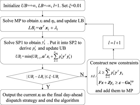
Figure 2. Flowchart of the solving algorithm for the two-stage RPS dispatch model.

5 Numerical tests

5.1 Basic settings

Numerical tests are carried out on a six-bus test system, the structure of which is shown in Figure 3. The parameters of the five thermal units are given in Table 1. The parameters of the seven transmission lines are given in the study by Jiang et al. (2012). Three wind farms, namely, WF1, WF2, and WF3, are connected to bus 4, bus 5, and bus 6, respectively. The predicted power curves of the total wind farm output and the system load excluding the FML are shown in Figure 3. Bus 3, bus 4, and bus 5 are load buses, peak load values of which are 196 MW, 98 MW, and 196 MW, respectively. The load buses are assumed to have a perfect positive correlation. The penalty prices of wind curtailment and load shedding are 100 $/MW and 500 $/MW, respectively.

Figure 3

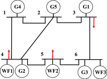
Figure 3. RPS structure.

Table 1

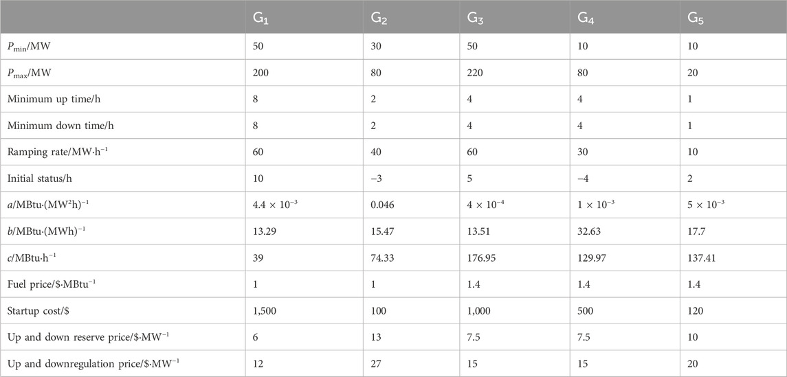
Table 1. Parameters of thermal units.

The historical prediction error data are obtained from the study by Cai (2024). According to the historical data, the extreme power outputs of the three wind farms are computed and shown in Figure 4.

Figure 4

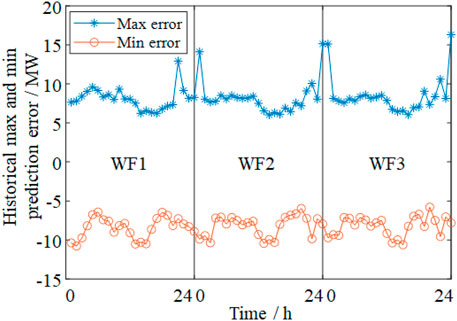
Figure 4. Maximum and minimum prediction errors at each hour of three wind farms in historical data.

The FML is connected to bus 3, the regulation parameters of which are shown in Table 2.

Table 2

Table 2. Regulation parameters of the FML.

The numerical tests are run on an Intel core i5-13500H personal computer with 32 GB RAM and solved using CPLEX 12.10 in MATLAB R2020b.

5.2 Comparison between ITSDRO with the existing RO and DRO methods

To demonstrate the performance of the ITSDRO method, the inscribed polyhedron-based RO (IPRO) in the study by Zhang et al. (2022) and the circumscribed polyhedron-based DRO (CPDRO) in the study by Zhang et al. (2021) are employed for comparison. All three methods are data-driven and need to construct the typical scenario set based on historical prediction error samples before formal optimization. For better presentation, only the typical scenarios in which the initial probability is non-zero are given in Figure 5.

Figure 5

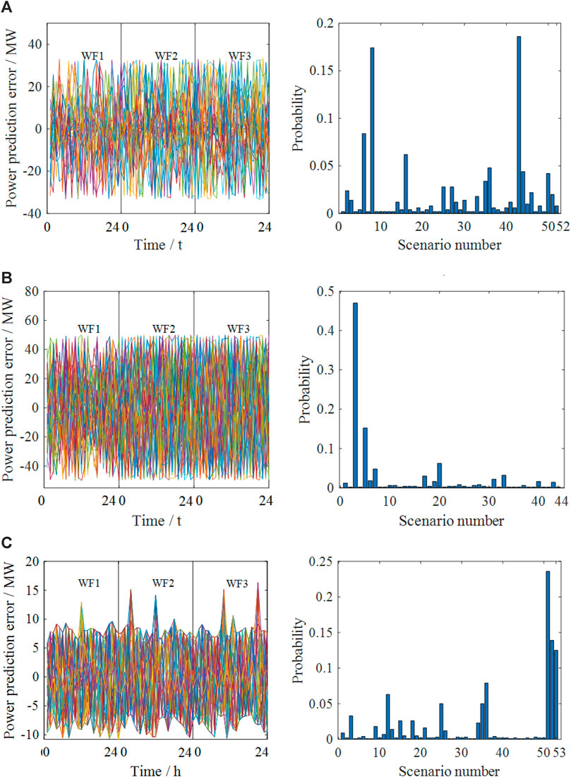
Figure 5. Comparison of the typical scenario sets of the three methods. (A) Typical scenarios and the corresponding probability of IPRO, (B) typical scenarios and the corresponding probability of CPDRO, and (C) typical scenarios and the corresponding probability of ITSDRO.

Figures 4, 5 show that the typical scenarios of the three methods are not simply located at the maximum or minimum prediction errors of the wind farms because of the spatiotemporal correlation between the prediction errors. However, IPRO and CPDRO directly adopt the vertices of the inscribed and circumscribed polyhedra of the MVEE as the typical scenario sets, respectively, in which some impossible scenarios exceed the limits of the prediction errors.

Then, the dispatch solutions of the three methods are shown in Figures 6–9. The corresponding dispatch costs of the test system optimized by the three methods are listed in Table 3.

Figure 6

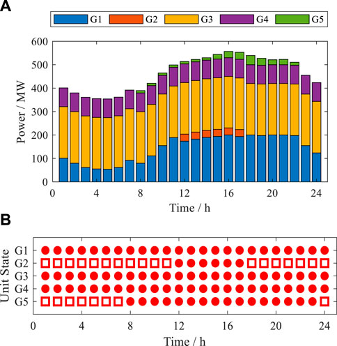
Figure 6. Day-ahead dispatch solution of the RPS by IPRO. (A) Scheduled power and (B) unit commitment.

Figure 7

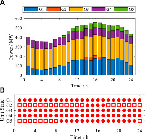
Figure 7. Day-ahead dispatch solution of the RPS by CPDRO. (A) Scheduled power and (B) unit commitment.

Table 3

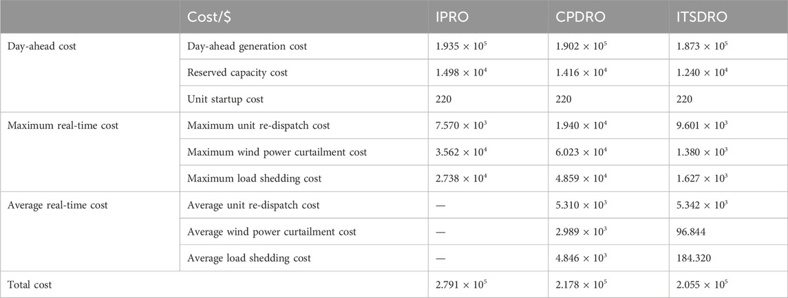
Table 3. Comparison of the dispatch costs optimized by the three methods.

Figures 6–9 and Table 3 show that

1) The solutions of the three methods can cope with all the uncertain scenarios they take into account, so they are all sufficiently robust.

2) The cost terms of the second stage are directly affected by the selected typical scenarios. IPRO and CPDRO only consider the extreme scenarios, while the uncertainty set of ITSDRO additionally contains the cluster centers. Since the re-dispatch costs of extreme scenarios are much higher than those of the cluster centers, the second-stage cost of ITSDRO is lower than that of the other two methods.

3) The cost terms of the first stage are indirectly affected by the selected typical scenarios. If only the extreme scenarios are taken into account in the DRO, the first-stage dispatch schemes will completely prepare for the extreme scenarios with very low probabilities and arrange too much reserve capacity, as shown in Figure 9. In this case, unit commitment schemes are also forced to be in the relatively uneconomic region. As an example, IPRO and CPDRO start up more units than ITSDRO in 8, 9, and 14 h, as shown in Figures 6–8.

4) In the absence of a targeted adjusting mechanism, these impossible scenarios of IPRO and CPDRO lead to conservative decisions and higher operation costs. As one of the RO methods, IPRO is more significantly affected because its solution is aimed at addressing the worst-case scenario. As one of the DRO methods, CPDRO is less affected because the initial probabilities of the impossible scenarios are much smaller than those of the other extreme scenarios.

Figure 8

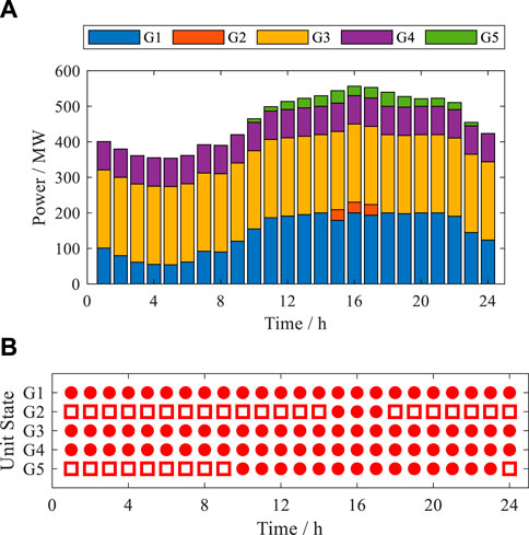
Figure 8. Day-ahead dispatch solution of the RPS by ITSDRO. (A) Scheduled power and (B) unit commitment.

Figure 9

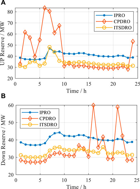
Figure 9. Total day-ahead reserved capacity of all units. (A) Up reserved capacity and (B) down reserved capacity.

The simulation results above are discussed below.

1) The second stage of a two-stage model is constructed to examine whether the RPS can sufficiently dispatch the flexible resources to cope with various scenarios including the extreme ones. However, most existing RO and DRO methods only consider extreme scenarios in the second stage, forcing the day-ahead dispatch to perform targeted preparation, which leads to redundancy in the flexible resource allocation and an increase in dispatch costs.

2) The proposed ITSDRO designs and employs an improved typical scenario set to reduce waste in the allocation of flexible resources without sacrificing the ability to cope with extreme scenarios. Therefore, the derived day-ahead dispatch scheme becomes more economical without the loss of robustness.

5.3 Validation of the DR of the FML

To validate the participation of the FML in the DR, two cases are designed for comparative analysis.

Case 1. Only conventional units are regarded as flexible resources in the second stage.

Case 2. Both conventional units and the DR of the FML participate in the re-dispatch in the second stage.

Based on the basic information given in Section 5.1, ITSDRO is performed to solve the two cases. The resulting dispatch costs are shown in Table 4, along with the amount of wind power curtailment and load shedding in the second stage.

Table 4 shows that, after the FML participates in DR projects, the maximum and average load shedding decrease by 13.32% and 15.17%, respectively, and the maximum and average wind power curtailment decrease by 10.33% and 0.41%, respectively. This indicates that the RPS becomes more flexible in coping with the power prediction error.

Figure 10 shows that the predicted wind power curve presents the anti-peak shaving characteristics. In load peak and valley periods, the FML can proactively decrease and increase its power consumption to reduce load shedding and wind curtailment amounts. From this perspective, since the DR of the FML plays the role of the regulation resource of RPS in the second stage, the reserved capacity in the first stage can be reduced accordingly. Therefore, the final total dispatch cost is decreased by 2.10%.

As shown in Figures 11 and 12, the wind curtailment is avoided and the load shedding amount is decreased even under the worst scenario, which verifies the effectiveness of the DR of the FML.

Table 4

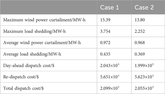
Table 4. Comparison of the dispatch results of case 1 and case 2.

Figure 10

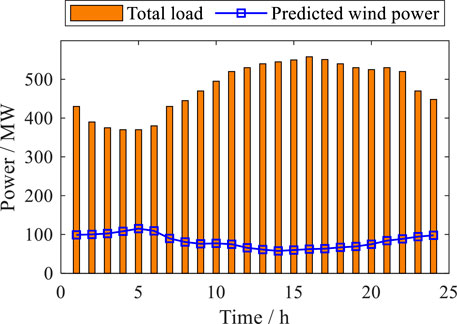
Figure 10. Predicted load and wind power.

Figure 11

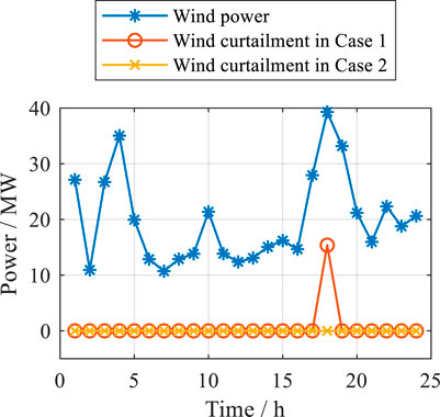
Figure 11. Wind curtailment in case 1 and case 2 under the worst scenario of wind curtailment.

Figure 12

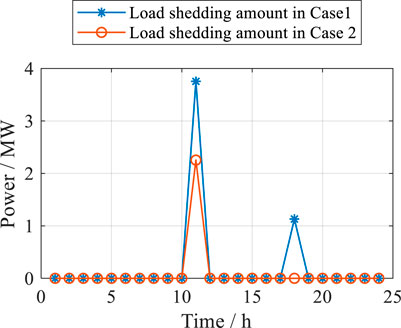
Figure 12. Load shedding amount in case 1 and case 2 under the worst scenario of load shedding.

6 Conclusion

This paper focuses on establishing the ITSDRO method, which is a two-stage co-dispatch method of energy and reserve for the RPS considering the DR of the FML. First, the FML is regarded as a flexible regulation resource, and its constraints for participating in DR projects are constructed. Then, an improved typical scenario set generation method is proposed with the spatiotemporal correlation between the power prediction errors considered. Based on this typical scenario set and the DRO theory, the ITSDRO model is formed and then solved by the column and constraint generation algorithm. Numerical tests are designed to verify the correctness and effectiveness of ITSDRO. According to the simulation results, some conclusions are drawn below.

1) An impossible extreme scenario identification and adjustment mechanism is proposed to address the feasibility issue of the existing inscribed and circumscribed polyhedron-based methods. Then, the extreme scenarios are united with cluster centers of the historical prediction error samples to form an improved typical scenario set with much lower conservativeness.

2) The two-stage ITSDRO dispatch model and corresponding solution method are proposed to optimize the co-dispatch strategy of energy and reserve for the RPS. The simulation results indicate that because of the utilization of the improved typical scenario set, the day-ahead dispatch cost can be reduced while keeping a small amount of load shedding and RES power curtailment.

3) The DR model of the FML is constructed and integrated into the ITSDRO dispatch model. The simulation results indicate that, with the proactive participation of the FML in the DR, the amount of load shedding and RES power curtailment is significantly decreased even under large prediction errors. This means that the flexibility of the RPS to cope with uncertainty is enhanced due to the DR of the FML.

Data availability statement

Publicly available datasets were analyzed in this study. This data can be found here: https://dx.doi.org/10.13140/RG.2.2.20878.98888.

Author contributions

JQ: writing–original draft, conceptualization, data curation, methodology, validation, and visualization. JC: writing–original draft, funding acquisition, software, supervision, and writing–review and editing. LH: conceptualization, funding acquisition, investigation, project administration, supervision, and writing–review and editing. ZM: conceptualization, formal analysis, resources, validation, and writing–review and editing.

Funding

The author(s) declare that financial support was received for the research, authorship, and/or publication of this article. This study was supported by the Natural Science Foundation of Jiangsu Province of China (BK20220340).

Conflict of interest

The authors declare that the research was conducted in the absence of any commercial or financial relationships that could be construed as a potential conflict of interest.

Publisher’s note

All claims expressed in this article are solely those of the authors and do not necessarily represent those of their affiliated organizations, or those of the publisher, the editors, and the reviewers. Any product that may be evaluated in this article, or claim that may be made by its manufacturer, is not guaranteed or endorsed by the publisher.

References

Balavand, A., Kashan, A. H., and Saghaei, A. (2018). Automatic clustering based on crow search algorithm-kmeans (CSA-Kmeans) and data envelopment analysis (DEA). Int. J. Comput. Int. Sys 11 (1), 1322–1337. doi:10.2991/ijcis.11.1.98

CrossRef Full Text | Google Scholar

Boldrini, A., Koolen, D., Crijns-Graus, W., Worrell, E., and van den Broek, M. (2024). Flexibility options in a decarbonising iron and steel industry. Renew. Sustain. Energy Rev. 189, 113988. doi:10.1016/j.rser.2023.113988

CrossRef Full Text | Google Scholar

Cai, J. Historical wind prediction error. Available at: https://dx.doi.org/10.13140/RG.2.2.20878.98888.2024; [Accessed 7 April 2024].

Google Scholar

Cai, J., Hao, L., Xu, Q., and Zhang, K. (2022). Reliability assessment of renewable energy integrated power systems with an extendable Latin hypercube importance sampling method. Sustain Energy Techn 50, 101792. doi:10.1016/j.seta.2021.101792

CrossRef Full Text | Google Scholar

Cai, J., and Xu, Q. (2021). Capacity credit evaluation of wind energy using a robust secant method incorporating improved importance sampling. Sustain Energy Techn 43, 100892. doi:10.1016/j.seta.2020.100892

CrossRef Full Text | Google Scholar

Carrion, M., and Arroyo, J. M. (2006). A computationally efficient mixed-integer linear formulation for the thermal unit commitment problem. Ieee T Power Syst. 21 (3), 1371–1378. doi:10.1109/tpwrs.2006.876672

CrossRef Full Text | Google Scholar

Chen, Z., Chen, Y., He, R., Liu, J., Gao, M., and Zhang, L. (2022). Multi-objective residential load scheduling approach for demand response in smart grid. Sustain Cities Soc. 76, 103530. doi:10.1016/j.scs.2021.103530

CrossRef Full Text | Google Scholar

Cheng, L., Zang, H., Trivedi, A., Srinivasan, D., Wei, Z., and Sun, G. (2024). Mitigating the impact of photovoltaic power ramps on intraday economic dispatch using reinforcement forecasting. Ieee T Sustain Energ 15 (1), 3–12. doi:10.1109/tste.2023.3261444

CrossRef Full Text | Google Scholar

Cheng, L., Zang, H., Wei, Z., and Sun, G. (2023). Secure multi-party household load scheduling framework for real-time demand-side management. Ieee T Sustain Energ 14 (1), 602–612. doi:10.1109/tste.2022.3221081

CrossRef Full Text | Google Scholar

de Chalendar, J. A., McMahon, C., Fuentes Valenzuela, L., Glynn, P. W., and Benson, S. M. (2023). Unlocking demand response in commercial buildings: empirical response of commercial buildings to daily cooling set point adjustments. Energ Build. 278, 112599. doi:10.1016/j.enbuild.2022.112599

CrossRef Full Text | Google Scholar

Derakhshandeh, S. Y., Hamedani Golshan, M. E., Ghazizadeh, M. S., and Sherkat Masoum, M. A. (2017). Stochastic scenario-based generation scheduling in industrial microgrids. Int. T Electr. Energy 27 (11), e2404. doi:10.1002/etep.2404

CrossRef Full Text | Google Scholar

Feizi, M. R., Khodayar, M. E., and Li, J. (2022). Data-driven distributionally robust unbalanced operation of distribution networks with high penetration of photovoltaic generation and electric vehicles. Electr. Pow. Syst. Res. 210, 108001. doi:10.1016/j.epsr.2022.108001

CrossRef Full Text | Google Scholar

Gao, H., Wang, R., Liu, Y., Wang, L., Xiang, Y., and Liu, J. (2020). Data-driven distributionally robust joint planning of distributed energy resources in active distribution network. Iet Generation, Transm. Distribution 14 (9), 1653–1662. doi:10.1049/iet-gtd.2019.1565

CrossRef Full Text | Google Scholar

Guo, L., Wang, X., Li, Z., and Li, W. (2023). Optimization of declared capacity for electrical fused magnesia furnaces participating in primary frequency control. Energy Rep. 9, 687–694. doi:10.1016/j.egyr.2023.05.104

CrossRef Full Text | Google Scholar

Huang, H., Zhou, M., Zhang, L., Li, G., and Sun, Y. (2019). Joint generation and reserve scheduling of wind-solar-pumped storage power systems under multiple uncertainties. Int. T Electr. Energy. 29 (7), e12003. doi:10.1002/2050-7038.12003

CrossRef Full Text | Google Scholar

Jiang, R., Wang, J., and Guan, Y. (2012). Robust unit commitment with wind power and pumped storage hydro. Ieee T Power Syst. 27 (2), 800–810. doi:10.1109/tpwrs.2011.2169817

CrossRef Full Text | Google Scholar

Karna, A., and Gibert, K. (2022). Automatic identification of the number of clusters in hierarchical clustering. Neural Comput. Appl. 34 (1), 119–134. doi:10.1007/s00521-021-05873-3

CrossRef Full Text | Google Scholar

Liu, H., Qiu, J., and Zhao, J. (2022). A data-driven scheduling model of virtual power plant using Wasserstein distributionally robust optimization. Int. J. Elec Power 137, 107801. doi:10.1016/j.ijepes.2021.107801

CrossRef Full Text | Google Scholar

Liu, J., Zang, H., Cheng, L., Ding, T., Wei, Z., and Sun, G. (2023). A Transformer-based multimodal-learning framework using sky images for ultra-short-term solar irradiance forecasting. Appl. Energ 342, 121160. doi:10.1016/j.apenergy.2023.121160

CrossRef Full Text | Google Scholar

Mazidi, M., Rezaei, N., and Ghaderi, A. (2019). Simultaneous power and heat scheduling of microgrids considering operational uncertainties: a new stochastic p-robust optimization approach. Energy (Oxford) 185, 239–253. doi:10.1016/j.energy.2019.07.046

CrossRef Full Text | Google Scholar

Saberi, H., Zhang, C., and Dong, Z. Y. (2021). Data-driven distributionally robust hierarchical coordination for home energy management. Ieee T Smart Grid 12 (5), 4090–4101. doi:10.1109/tsg.2021.3088433

CrossRef Full Text | Google Scholar

Shui, Y., Gao, H., Wang, L., Wei, Z., and Liu, J. (2019). A data-driven distributionally robust coordinated dispatch model for integrated power and heating systems considering wind power uncertainties. Int. J. Elec Power 104, 255–258. doi:10.1016/j.ijepes.2018.07.008

CrossRef Full Text | Google Scholar

Tan, W. S., Shaaban, M., and Ab Kadir, M. Z. A. (2019). Stochastic generation scheduling with variable renewable generation: methods, applications, and future trends. Iet Generation, Transm. Distribution 13 (9), 1467–1480. doi:10.1049/iet-gtd.2018.6331

CrossRef Full Text | Google Scholar

Trojani, A. G., Moghaddam, M. S., and Baigi, J. M. (2023). Stochastic security-constrained unit commitment considering electric vehicles, energy storage systems, and flexible loads with renewable energy resources. J. Mod. Power Syst. Cle. 11 (5), 1405–1414. doi:10.35833/mpce.2022.000781

CrossRef Full Text | Google Scholar

Wang, J., Wang, Q., and Sun, W. (2023). Quantifying flexibility provisions of the ladle furnace refining process as cuttable loads in the iron and steel industry. Appl. Energ 342, 121178. doi:10.1016/j.apenergy.2023.121178

CrossRef Full Text | Google Scholar

Wang, L., Jiang, C., Gong, K., Si, R., Shao, H., and Liu, W. (2020). Data-driven distributionally robust economic dispatch for distribution network with multiple microgrids. Iet Generation, Transm. Distribution 14 (24), 5712–5719. doi:10.1049/iet-gtd.2020.0861

CrossRef Full Text | Google Scholar

Xie, J., Ajagekar, A., and You, F. (2023). Multi-Agent attention-based deep reinforcement learning for demand response in grid-responsive buildings. Appl. Energ 342, 121162. doi:10.1016/j.apenergy.2023.121162

CrossRef Full Text | Google Scholar

Yang, Q., Wang, J., Liang, J., and Wang, X. (2024). Chance-constrained coordinated generation and transmission expansion planning considering demand response and high penetration of renewable energy. Int. J. Elec Power 155, 109571. doi:10.1016/j.ijepes.2023.109571

CrossRef Full Text | Google Scholar

Yuan, C., and Yang, H. (2019). Research on K-value selection method of K-means clustering algorithm. J 2 (2), 226–235. doi:10.3390/j2020016

CrossRef Full Text | Google Scholar

Zhang, Y., Liu, Y., Shu, S., Zheng, F., and Huang, Z. (2021). A data-driven distributionally robust optimization model for multi-energy coupled system considering the temporal-spatial correlation and distribution uncertainty of renewable energy sources. Energy 216, 119171. doi:10.1016/j.energy.2020.119171

CrossRef Full Text | Google Scholar

Zhang, Y., Yang, J., Pan, X., Zhu, X., Zhan, X., Li, G., et al. (2022). Data-driven robust dispatch for integrated electric-gas system considering the correlativity of wind-solar output. Int. J. Elec Power 134, 107454. doi:10.1016/j.ijepes.2021.107454

CrossRef Full Text | Google Scholar

Zheng, X., Zhou, B., Wang, X., Zeng, B., Zhu, J., Chen, H., et al. (2023). Day-ahead network-constrained unit commitment considering distributional robustness and intraday discreteness: a sparse solution approach. J. Mod. Power Syst. Cle 11 (2), 489–501. doi:10.35833/mpce.2021.000413

CrossRef Full Text | Google Scholar

Nomenclature