Optimized LSTM for Accurate Smart Grid Stability Prediction Using a Novel Optimization Algorithm

The stability of smart grids is crucial for ensuring reliable and efficient power distribution in modern energy systems. This paper presents an optimized Long Short-Term Memory model for predicting smart grid stability, leveraging the Novel Guide-Waterwheel Plant Algorithm (Guide-WWPA) for enhanced performance. Traditional methods often struggle with the complexity and dynamic nature of smart grids, necessitating advanced approaches for accurate predictions. The proposed LSTM model, optimized using Guide-WWPA, addresses these challenges by effectively capturing temporal dependencies and nonlinear relationships in the data. The proposed approach involves a comprehensive preprocessing pipeline to handle data heterogeneity and noise, followed by the implementation of the LSTM model optimized through Guide-WWPA. The Guide-WWPA combines the strength of the WWPA with a novel guidance mechanism, ensuring efficient exploration and exploitation of the search space. The optimized LSTM is evaluated on a real-world smart grid dataset, demonstrating superior performance compared to traditional optimization techniques. Experimental Results indicate significant improvements in prediction accuracy and computational efficiency, highlighting the potential of the Guide-WWPA optimized LSTM for real-time smart grid stability prediction. This work contributes to the development of intelligent energy management systems, offering a robust tool for maintaining grid stability and enhancing overall energy reliability. On the other hand, statistical evaluations were carried out to prove the stability and difference of the proposed methodology. The results of the experiments demonstrate that the Guide-WWPA + LSTM strategy is superior to the other machine learning approaches.

1 Introduction

Both traditional grids, which consisted of small generation centers that supplied energy to customers, and renewable energy came into existence as a result of the expansion in population across the world, which led to an increase in the amount of power that was used. The proliferation of renewable energy, on the other hand, has resulted in the emergence of a hybrid of these two that is known as ”prosumers,” which both provide and consume energy (Siddiqui et al., 2017). These prosumers, on the other hand, require the flow of energy in a grid to be in both directions. The delivery, generation, and use of energy are all more complicated for these prosumers, as well. In light of this, the financial implications that are associated with prosumers and renewable energy have grown increasingly difficult to manage, particularly with regard to the decision of whether or not to purchase energy at a cost that is already known (Bajaj and Singh, 2020). Furthermore, this research on the stability of smart grids has received a substantial amount of attention (Panda et al., 2022). To facilitate the development of a system that is capable of efficiently distributing power, smart grids can collect data pertaining to users. The deployment of additional power plants for the purpose of dissipating electricity is reduced as a result of the implementation of smart grids (Kumar et al., 2016; Mahmud et al., 2020; Kumar et al., 2022). Additionally, smart grids make use of renewable energy resources in order to become secure when they are hooked into a grid in order to get an additional source of electricity. The use of smart grids has the potential to significantly lower the cost of power and simultaneously lower pollution levels. These grids then obtain a cost value for the power and convey this cost information to the clients so that they may make decisions regarding their usage. After receiving information from consumers, these grids assess the information with regard to the current supply information. The capacity to forecast the stability of a smart grid is one of the most important requirements for such systems. This is because the process is reliant on the passage of time.

Deep neural networks (Alazab and Tang, 2019; Vinayakumar et al., 2019; Irshad et al., 2020) and machine learning (Shafiq et al., 2018; Iwendi et al., 2020) are two examples of artificial intelligence applications that have brought about a revolution in the process of energy generation and distribution. In addition to this, it was a crucial factor in the forecast of the stability of the smart grid for residential loads (Hong et al., 2020). Recurrent neural networks, have been suggested as a promising method for precisely forecasting the stability of smart grids (Adil et al., 2020). The problem of low accuracy is effectively addressed by feed-forward neural networks, which develop and implement effective solutions. Image processing (Szegedy et al., 2014) and speech recognition (Yu and Deng, 2015) are two examples of applications that have already demonstrated the feasibility of these neural networks. Additionally, they are relevant for forecasting the stability of smart grids. It is abundantly evident that numerous interactions take place between power sources, distribution stations, and a variety of entities, including smart cities, electric cars, industries, and smart buildings (Alazab et al., 2020Alazab et al., 2020). The research suggests that smart grids make use of a wide variety of artificial intelligence approaches, including deep learning, machine learning, and artificial neural networks, in order to implement energy consumption strategies that are more efficient. There were a number of different deep learning algorithms that were presented in (Jindal et al., 2016) for the purpose of predicting electricity demands for a smart grid. The focus of the writers is on the employment of a variety of deep learning technologies for load prediction in smart grids. Additionally, they compared the accuracy results for the developed applications in terms of the mean absolute error and the root-mean-square error. Based on the results that were obtained, they concluded that CNN with the k-means algorithm had a significant percentage of minimizing the RMSE during the process.

The cost of electricity greatly impacts the stability of the electrical networks. The stability parameter of smart grids is also affected by the reaction times of power consumers and providers. Wood provided a mathematical model for DSGC systems in (Razavi et al., 2019), which correlates the cost of power to changes in the frequency of grids based on time measurements of a few seconds. The purpose of this model was to show the demand control of smart grids. We simulated the power demand-side production and consumption based on analog time gauges, we created a machine learning technique that corresponded to the data, and we determined that the variables that were employed were independent. When training the algorithm with massive amounts of data that change their dimensions, the accuracy of the algorithm is reduced. Through the use of a principal component analysis technique (Pham et al., 2020), Chen suggested a machine learning algorithm in (Kotb et al., 2019) with the goal of reducing the dimensions of the data that is employed in order to improve the stability of smart grids. A number of artificial intelligence algorithms have been developed for the purpose of predicting the stability of smart grids. In the article (Iwendi et al., 2021), the authors suggested a classification and regression trees method for the purpose of predicting the stability of smart grid operation. An overall accuracy of 80% was reached by the authors through the utilization of a four-node star topology for a simulated DSGC system. A decision tree method with a significantly simplified design was given by the authors in (Din et al., 2019) for the purpose of predicting the stability of smart grid power systems. This method was implemented on the power system that consisted of 39 buses. Using six different samples from the dataset, it was able to attain an accuracy rate of 83%.

An accuracy of 89.22% was attained by the CNN that was presented by the authors in (Ahmed et al., 2019) for the purpose of predicting the stability of a smart grid. The CNN was tested on the IEEE 118-bus and 145-bus systems. Several different assessment measures were utilized in order to assess the quality of this work. Using the Bayesian rate algorithm, the authors of (Xiang et al., 2023) devised a method for predicting the stability of smart grid operation. However, this approach required an excessive amount of computing time for the training procedure, despite the fact that it was also applied to the IEEE 39-bus test system and achieved an accuracy of 91.6%. For the purpose of predicting the stability of a smart grid with a high number of data features, the authors of (Ghorbanian et al., 2019) presented an XGBoost algorithm that used inertial sensors. This method was utilized on a power system consisting of 39 buses, and it achieved an accuracy rate of 97%. For the purpose of assessing the effectiveness of the algorithm that was constructed, however, just one assessment parameter, specifically accuracy, was applied. Additionally, real-time modeling of power systems may be utilized for a variety of smart grid models (Zhang et al., 2018; Moldovan and Salomie, 2019; Syed et al., 2020; Jin et al., 2023; Shrivastava and Yadav, 2023). A lot of research projects have attempted to construct an accurate neural network for smart grid stability prediction; nevertheless, there are still improvements that need to be attained, according to the literature that has been examined. This is something that may be argued. With the ultimate goal of raising or improving the forecast accuracy of the neural network through the use of a hyperparameter tuning approach, a neural network is presented in this research as a means of predicting the resilience of smart grids. On the dataset that is accessible through the Kaggle repository, the neural network is practiced and evaluated (Bassamzadeh and Ghanem, 2017).

Through the classification of the smart grid dataset obtained from the UCI machine learning repository, a novel optimized LSTM model is proposed in this article. The model’s purpose is to predict the stability of smart grids. The findings of the experiments are then contrasted with more contemporary machine learning algorithms and optimization methods. The main contributions of this work are listed in the following:

$•$ A novel optimization algorithm is proposed based on a novel modification denoted by Guide-WWPA.

$•$ The proposed Guide-WWPA is used to optimize SMOTE for better selection of the synthetic samples to boost the overall performance of the prediction of smart grid stability.

$•$ The proposed Guide-WWPA is binarized and denoted by (bGuide-WWPA) to solve the problem of feature selection applied to the adopted dataset.

$•$ In order to evaluate the effectiveness of the bGuide-WWPA method that has been presented for feature selection, the implementation of a set of computational analytic measures is realized.

$•$ The continuous version of the Guide-WWPA is used to optimize the parameters of the LSTM model for improving the prediction accuracy of smart grid stability.

The remainder of the manuscript is structured as follows: The research that has been done before on the smart grid stability prediction is discussed in Section 2. More information on the methodology that has been proposed is found in Section 3. In Section 4, the experimental process that was used to evaluate the proposed method is presented and discussed. Section 5 presents the conclusion of this work as well as a view on its potential future directions.

2 Literature Review

With the potential to directly reduce the availability and safety measures of a smart grid, a covert data integrity attack on a communications network might potentially be dangerous (Hafeez et al., 2020a; Hafeez et al., 2020b; Hafeez et al., 2021). It is possible for this attack to challenge the integrity of the data and to cause a false evaluation of the status, both of which would have a devastating impact on the entire power system process. This attack is carefully deployed in order to escape the typical bad data detectors that are found in power control stations (Hafeez et al., 2020c; Hafeez et al., 2020d; Nawaz et al., 2020). An intelligent system is developed by the authors of (Ahmed et al., 2019) to identify stability in smart grids by making use of non-labeled data. This system is based on an unsupervised machine-learning application. To construct the smart grid, numerous information and communication technologies are utilized, which results in enormous amounts of data coming from a variety of sources. It is possible to overcome the difficulty of processing and managing the enormous volume of data by utilizing intelligent systems and big data analysis (Xiang et al., 2023) in smart grid systems. The article (Ghorbanian et al., 2019) highlights a number of difficulties that are linked to the utilization of big data analysis in smart grids.

In light of the fact that the information used for the verification of membership may result in instabilities in the grid, the assessment of the stability of the smart grid is a research challenge that is particularly difficult to solve. This allows for setups to be governed in such a way that the grid remains stable regardless of any irregularities that may occur. Using feature extraction as a basis, the authors of (Moldovan and Salomie, 2019) investigate the use of a machine learning method for the purpose of forecasting the stability of smart grids. For the feature selection process, the authors of this paper make use of three different methods: Multivariate Adaptive Regression Splines, Binary Kangaroo Mob optimization Features Selection, and Binary Particle Swarm optimization Features Selection. Classifiers such as Logistic Regression, Random Forest, Gradient Boosted Trees, and Multilayer Perceptron Classifier are utilized in order to predict the stability of the grid that is accurate.

In the past, electrical grids consisted of communication that only went in one direction between the infrastructure and the end users. Despite the fact that these grids were installed all over the world, there remained a large amount of worry over the effectiveness of power management. The evolution of smart grids, which include communication in both directions between the grid and the customer, was motivated by the need to address this difficulty. The development of this smart grid was primarily motivated by the desire to properly forecast the kinds of energy that a particular population will consume. For the purpose of making forecasts, machine learning algorithms are implemented with the use of information such as historical weather, load, and energy generation data (Jin et al., 2023). The researchers also built two models, which are referred to as the deep neural network model and the linear regression model (Shrivastava and Yadav, 2023). The root mean squared error was used to evaluate these models, and the results showed that the deep neural network models performed better than the linear regression models when it came to predicting the amount of load and energy output in a specifically designated area. Within the context of the smart grid, energy load prediction refers to the process of anticipating the electrical power requirements in order to satisfy dynamic demands. In order to assist electrical services in monitoring their energy generation and process, there is an urgent requirement to incorporate predictive accuracy for load. At the moment, the majority of the prediction in any system is carried out by means of machine learning algorithms in order to attain the highest possible level of effectiveness. For the purpose of predicting the energy demand, large data frameworks such as Apache Spark and Apache Hadoop (Syed et al., 2020; Almetwally and Meraou, 2022) have been offered as available options. Other regression approaches, such as linear regression, modified linear regression, decision tree, random forest, and gradient-boosted trees, are evaluated by the authors using MLib to determine how accurate their predictions are.

The implementation of power systems that are able to regulate the dissipation of energy effectively is now being driven by the trend of smart grids. The utilization of artificially intelligent systems is helpful in simplifying the process of deploying a smart grid network, which is notoriously difficult owing to the enormous amount of data that is being produced. Learning techniques such as DL, reinforcement learning, and deep reinforcement learning have been made possible as a result of the progress that has been made in the evolution of intelligent systems. For the purpose of enabling future academics to do more study, the difficulties that need to be overcome in order to implement these technologies in smart grids are mentioned (Zhang et al., 2018; Muhammed and Almetwally, 2024). The fluctuating energy consumption of home appliances is a significant issue that has to be addressed in order to ensure the sustainability and effectiveness of the construction of smart cities. The development of Internet of Things technology has made it possible to use additional energy management strategies in order to deal with the ever-changing energy consumption. When it comes to consumption prediction in occupied buildings, the authors of (Bassamzadeh and Ghanem, 2017) propose the deployment of a probabilistic data-driven prognostic approach. The system is able to discover dependency links among the contributing variables thanks to the utilization of a Bayesian Network architecture, which is utilized by this approach. Using the datasets that were provided by Pacific Northwest National Lab and that were compiled through a pilot Smart Grid project, the authors evaluate the proposed method.

The issues that smart grids face and the requirements that they will have in the future have prompted a consortium to be formed by a number of large corporations. Artificial Neural Networks, Machine Learning, and DL are some of the Artificial Intelligence techniques that smart grids employ in order to achieve efficient energy usage. With regard to the smart grid, (Almalaq and Edwards, 2017) proposes a variety of different DL algorithms for load prediction problems. Within the context of the smart grid network, the authors concentrate on the utilization of various applications of deep learning for load prediction. In addition, the authors examine the accuracy results of Root Mean Square Error and Mean Absolute Error for the applications that were investigated. Based on their findings, they conclude that the utilization of a convolutional neural network in conjunction with the k-means method resulted in a significant reduction in the root mean square error proportion. When it comes to the stability of distributed power networks, the price of electricity has a considerable influence. Many other factors affect the stability factor, such as the cost sensitivity and reaction times of power providers and consumers. By connecting the price of electricity to fluctuations in grid frequency over a time scale of a few seconds, authors in (Wood, 2020) proposed a model that is referred to as DSGC. This approach is intended to deliver demand-side control of distributed power grids. On similar time gauges, the authors performed a simulation of the power demand-side consumption and production. For the purpose of achieving dynamic grid stability for the simulation based on its independent variables, the authors additionally designed an improved data-matching machine-learning technique known as the transparent, open box learning network. When training a machine learning model with a large amount of data that has fluctuations in the dimensionality, the efficacy of the model is reduced accordingly. In order to decrease the number of dimensions of the data, the authors of (Chen, 2019) devise a secondary principal component analysis technique (Reddy et al., 2020). Increasing the stability of grid systems is accomplished by the application of this approach, which is used to regulate machine learning techniques. According to this review, it can be noted that there is no approach that is completely meet the stability difficulties in a smart grid network and predict its stability accurately. Therefore, in this research a novel approach is proposed to boost the prediction accuracy of smart grid stability using metaheuristic optimization.

3 The Proposed Methodology

This section describes the methodology proposed to boost the prediction accuracy of smart grid stability. The proposed method is based mainly on a novel modification to the WWPA algorithm, denoted by Guide-WWPA. This algorithm is used for feature selection and optimization of the LSTM hyperparameters. In the first step of the proposed methodology, the dataset about the electrical system that is compiled from the various power-generating units is completed. Normalization of the dataset is then performed using the min-max normalization method. The maximum and minimum values of the data are acquired and then substituted by applying Equation 1.

$\begin{array}{cc}\hfill \widehat{L}& =\frac{l-min\left(X\right)}{max\left(X\right)-min\left(X\right)}\hfill \\ \hfill & *\left(new\_min\left(X\right)-new\_max\left(X\right)\right)\hfill \\ \hfill & +new\_min\left(X\right)\hfill \end{array}(1)$

where $min(X)$ and $max(X)$ are notations that indicate the minimum and maximum values of the attributes in the provided dataset, respectively. In this context, $X$ stands for an attribute that is an element of the dataset. $New\_max(X)$ and $new\_min(X)$ describe the upper and lower boundary values in the provided range, respectively. $L$ represents the updated value of each item in a dataset, while $l$ relates to the values that were present in the dataset before. In addition, the dataset is balanced using the synthetic minority oversampling technique (SMOTE) which is optimized based on the proposed optimization methodology which is presented in the next section.

On the other hand, the machine learning algorithms are unable to handle the category values that are contained in the dataset. Label encoding is a technique that turns the category values in the dataset into numerical values that are appropriate for processing by machine learning algorithms. This is the reason why it is used. In the subsequent stage, the dataset comprising the smart grid is trained using the optimized LSTM technique that has been described. Several measures such as accuracy, precision, recall, and F1-score are used to evaluate the performance of the proposed model in comparison to other models, including classic LSTM, SVM, KNN, DT, MLP, and RF models. Detailed explanations of these models are provided in the following paragraphs. The coming sections present more details about the key steps of the proposed methodology.

3.1 Synthetic Minority Oversampling Technique (SMOTE)

The SMOTE method is a strategy that is used to oversample the minority classes in order to get a balanced dataset as proposed by authors in (Chawla et al., 2002). Through the process of interpolation and the selection of a neighbour from a minority class, the primary objective is to bring about fresh minority samples. Instead of only copying samples from minority classes, this method is able to generate synthetic sample data through its use. Because of this, the overfitting problem may be avoided with this strategy. This is how the SMOTE algorithm is supposed to be described. At the beginning of the process, a point $x$ is chosen at random from the minority class sample, and then its $k$ nearest neighbours are obtained from other minority samples. Next, select one minority class sample from each of the $k$ neighbours and multiply it by one. A new synthetic sample, denoted by $xnew$, is generated in the vector that lies between $x$ and $x1$ by the utilisation of an interpolation technique during the last step. After careful consideration, one can reach the conclusion that the mathematical formulation of SMOTE is represented by Equation 2:

$X_{\mathit{new}}=X+\left(\widehat{X}-X\right)\times rand\left(\mathrm{0,1}\right)(2)$

A random integer between 0 and 1 is denoted by the expression $rand(\mathrm{0,1})$. In order to enhance the total number of minority class samples, the process described above is then repeated based on the beginning of the set of oversampling rates. Additionally, the SMOTE method is used to add a new minority class sample to the initial training samples. When viewed from a geometric point of view, this approach may be seen as an interpolation between two samples of minority classes. The classifier is able to generate more accurate predictions for samples of unknown minority classes as a result of this expansion of the decision space for the minority class. It is possible to prevent overfitting issues by using the SMOTE approach, which is both effective and straightforward in the generation of synthetic samples. Our databases contain a very small number of positive samples. The SMOTE technique was carried out after the five-fold cross-division in order to increase the number of positive samples in the training dataset. The final step is to feed the newly acquired training dataset into the classifier for the purpose of classification, and then to retrieve the results of the prediction. An illustration of the SMOTE method is shown in Figure 1. In this figure, the red circles represents the minority class samples and the dashed squares represents the majority class samples. The target of SMOTE is to increase the samples of the minority class to be equal to the number of samples in the majority class. This can be achieved by synthesizing the new class samples, small green circles.

Figure 1

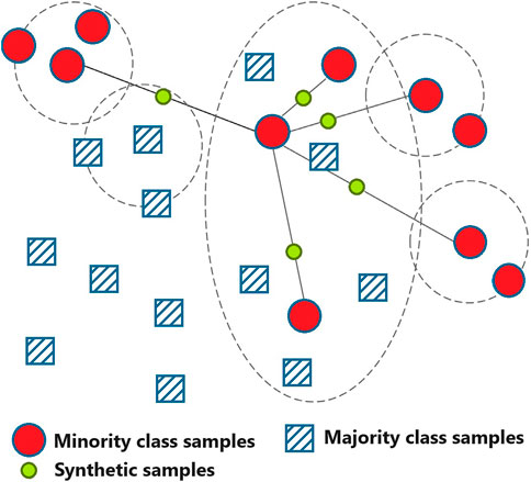
Figure 1. The schematic of SMOTE algorithm.

In this work, the synthetic samples generated by the SMOTE algorithm are optimized using the proposed optimization algorithm. This optimization enables generating the best set of samples that balance the dataset with boosting the overall performance of prediction process.

3.2 Long Short-Term Memory (LSTM)

The LSTM network has emerged as one of the most prominent strategies for overcoming this difficulty, according to an analysis of current research (Sutskever et al., 2014). A chain structure that contains many neural network modules is a characteristic of LSTM. An illustration of the architecture of LSTM may be found in Figure 2. This architecture is comprised of several gates, such as an input gate, an output gate, and a forget gate. The information that is being transmitted via the network is selected and rejected by these gates. Input gate $i(t)$ is made up of $tanh$, which is an activation function that ranges from $-1$ to 1. Processing requires the current input $x(t)$, as well as the parameters $C(t-1)$ and $h(t-1)$. It is important to remember that the activation function of gate $f(t)$ is a $sigmoid$ and $tanh$. The forget gate is responsible for determining the amount of information that must be kept from the output that came before it. In the event that the value is 1, the data will be translated into the network; yet, in the event that the value is 0, the data will not be sent through the network. The activation function of the output gate $o(t)$ is denoted by the $sigmoid$ function, which ranges from $-1$ to 1. Equations 3-5 are utilized in order to compute $i(t)$, $o(t)$, and $f(t)$ at each timestamp.

$i^{\left(t\right)}=\sigma \left(W^i\left[C^{\left(t-1\right)},h^{\left(t-1\right)},x^{\left(t\right)}\right]+b^i\right)(3)$

$o^{\left(t\right)}=\sigma \left(W^o\left[C^{\left(t-1\right)},h^{\left(t-1\right)},x^{\left(t\right)}\right]+b^i\right)(4)$

$f^{\left(t\right)}=\sigma \left(W^f\left[C^{\left(t-1\right)},h^{\left(t-1\right)},x^{\left(t\right)}\right]+b^i\right)(5)$

Figure 2

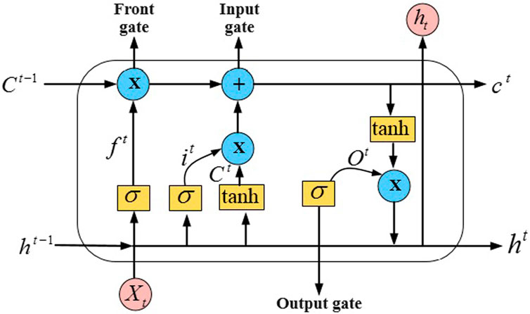
Figure 2. The structure of a typical LSTM model.

In this work, One LSTM is utilized for scanning in the upward and downward directions, while the second LSTM is used for scanning in the right and left directions. While traditional LSTM operates in both directions, this research makes use of two LSTMs. Specifically, the input of the second LSTM is a summation of the input of the first LSTM.

3.3 Waterwheel Plant Algorithm (WWPA)

WWPA is a novel approach to stochastic optimization that was conceived of in (Abdelhamid et al., 2023) and drew inspiration from the functioning of natural systems. A core concept that has been established for the Guide-WWPA is based on the assumption that it is possible to model the natural behavior of the waterwheel plant when it is engaged in the process of hunting. As the major source of inspiration for the core concept of Guide-WWPA, the approach that waterwheel plants use to detect their insect prey, catch it, and then transfer it to a more accessible spot before digesting it served as the key source of inspiration. We will talk about the concepts that led to the development of the algorithm in the next part, as well as the mathematical model that was used to describe the program’s methods.

3.3.1 The WWPA Inspiration

Small, translucent structures that resemble flytraps are seen on the broad petiole of the Waterwheel plant, which is formally referred to as Aldrovanda vesiculosa. As a means of preventing damage or unintentional activation, these traps, which measure around one-twelfth of an inch in size, are surrounded by bristle-like hairs. When the trap is closed around its victim, the hook-shaped teeth that are located on the outside edges of the trap interlock with one another, just like the teeth that are found on a flytrap. Around forty elongated trigger hairs, which are similar to those seen in Venus’s flytraps, are located inside the trap. These trigger hairs are responsible for causing the trap to close automatically. An additional feature of the plant is the presence of glands that secrete acid, which facilitates digestion. Once the unfortunate victim has been seized, it is successfully trapped and directed toward the base of the trap at the hinge by means of interlocking teeth and a mucus sealant. This process is repeated until the prey is completely trapped. The majority of the nutrients that are contained in the prey are absorbed by the trap when it digests the residual water. Similar to a flytrap, an Aldrovanda trap can collect and devour anywhere from two to four meals before it shuts down.

3.3.2 The Mathematical Model of WWPA

The WWPA algorithm is an iterative approach that calls for a population of persons to search for an optimal solution within the huge space of potential solutions. This search is carried out in order to get the best feasible solution. Particular values are assigned to the problem variables for every individual member of the WWPA population, which is symbolized by a waterwheel. The location of the waterwheel determines these values within the search area. Consequently, each waterwheel functions as a vector-based solution inside the system. It is the collection of waterwheels that the WWPA is represented by Equations 6, 7.

$P=\left[\begin{array}{c}{P}_1\\ ⋮\\ P_i\\ ⋮\\ P_N\end{array}\right]=\left[\begin{array}{ccccc}{p}_{1,1}& \cdots & p_{1,j}& \cdots & p_{1,m}\\ ⋮& \ddots & ⋮& ⋰& ⋮\\ p_{i,1}& \cdots & p_{i,j}& \cdots & p_{i,m}\\ ⋮& ⋰& ⋮& \ddots & ⋮\\ p_{N,1}& \cdots & p_{N,j}& \cdots & p_{N,M}\end{array}\right](6)$

$p_{i,j}=l{b}_j+r_{i,j}.\left(u{b}_j-l{b}_j\right),i=\mathrm{1,2},\dots ,N,j=\mathrm{1,2},\dots ,m(7)$

The number of waterwheels is denoted by the letter $N$ in this context, whereas the number of variables is denoted by the letter $m$. The random number that corresponds to the value $r_{i,j}$ is a number that falls anywhere between 0 and 1. The lowest and highest bounds of the j-th variable in the problem are denoted by the symbols $l{b}_j$ and $u{b}_j$, respectively. The population matrix, which includes the addresses of the waterwheels, is denoted by the letter $P$. The value of the j-th variable for the i-th waterwheel is denoted by the formula $p_{i,j}$, and each row $P_i$ in the matrix indicates a potential solution to the problem. It is feasible to evaluate the objective function of each waterwheel since each one of them is regarded to be a potential solution to the problem. A vector may be used to effectively represent the values that make up the objective function of the issue, as was established by previous research as being possible to use. Guide-WWPA population, which is a matrix of ten. A method that is given in the following equation is used to randomly decide the placements of the waterwheels in the search space. This is done in order to start the process.

$F=\left[\begin{array}{c}\hfill F_1\hfill \\ \hfill ⋮\hfill \\ \hfill F_i\hfill \\ \hfill ⋮\hfill \\ \hfill F_N\hfill \end{array}\right]=\left[\begin{array}{c}\hfill F\left(X_1\right)\hfill \\ \hfill ⋮\hfill \\ \hfill F\left(X_i\right)\hfill \\ \hfill ⋮\hfill \\ \hfill F\left(X_N\right)\hfill \end{array}\right](8)$

Using vector F in Equation 8, which includes all of the values of the objective function, we are able to estimate the value of the i-th waterwheel. Objective functions are evaluated and analyzed to determine which solutions are the best. Based on this, the candidate solution that is considered to be the best is linked to the greatest value of the objective function, while the member that is considered to be the worst is linked to the lowest value. The ideal solution is subject to change with each iteration due to the fact that the waterwheels move around the search area at varying rates. Waterwheels have a highly developed sense of smell, which enables them to successfully track and find pests they encounter throughout the process of exploration. This gives them a strong instinct to hunt. When a bug comes into the region of the waterwheel, it immediately begins to attack and then continues to pursue the target by precisely determining where it is located. In order to represent the first step of its population update process, the WWPA models this behavioral pattern of hunting. Through the incorporation of the waterwheel’s attack on the insect, the WWPA makes it more capable of exploring the ideal zone and avoiding becoming stuck in the local optimal region. As a consequence of this modeling methodology, major positional adjustments take place inside the search space. It is necessary to employ an equation in conjunction with a simulation of the waterwheel’s approach to the insect in order to compute the new location of the waterwheel using this method. By doing so, it is possible to ascertain the new position. Suppose the value of the goal function is increased by shifting the waterwheel to this new position. In that case, the location that was previously mentioned will no longer be employed in favor of the one that has been presented more straightforwardly, as represented by Equations 9, 10.

$\vec{W}={\vec{r}}_1.\left(\vec{P}\left(t\right)+2K\right)(9)$

$\vec{P}\left(t+1\right)=\vec{P}\left(t\right)+\vec{W}.\left(2K+{\vec{r}}_2\right)(10)$

Using Equation 11, one is able to make adjustments to the location of the waterwheel in the case that the result does not improve after three iterations in a row.

$\vec{P}\left(t+1\right)=Gaussian\left({\mu }_P,\sigma \right)+{\vec{r}}_1\left(\frac{\vec{P}\left(t\right)+2K}{\vec{W}}\right)(11)$

With values ranging from 0 to 2 and 0 to 1, respectively, the variables ${\vec{r}}_1$ and ${\vec{r}}_2$ are examples of random variables that are included in this context. Furthermore, $K$ is a variable that has values that range from 0 to 1, making it an exponential variable. The waterwheel plant will examine possible promising regions inside a circle that has a diameter of $\vec{W}$, which serves as the vector for the circle.

As part of the process of exploitation, the population is updated in WWPA, which is modeled by the way waterwheels capture and transport insects to a feeding tube based on their behavior. As a result of this simulated behavior, the exploitation capacity of WWPA is improved during the local search. This makes it possible for the algorithm to converge on better solutions that are relatively near to those that have been identified in the past. The placement of the waterwheel inside the search space is subject to certain minute alterations as a consequence of modeling the process of transferring the insect to the appropriate tube. The architects of the WWPA first choose a fresh, arbitrary position for each waterwheel in the population. This process is done in order to imitate the natural behavior of waterwheels. A ”good position for consuming insects” is what this particular place is referred to be. Following that, the waterwheel is moved to this new location, which replaces the previous location, in accordance with Equations 12, 13 if the value of the goal function is higher at this new location.

$\vec{W}={\vec{r}}_3.\left(K{\vec{P}}_{\mathit{best}}\left(t\right)+r_3\vec{P}\left(t\right)\right)(12)$

$\vec{P}\left(t+1\right)=\vec{P}\left(t\right)+K\vec{W}(13)$

A random variable with values ranging from 0 to 2 is denoted by the variable ${\vec{r}}_3$ in this scenario. The current solution at iteration $t$ is denoted by the symbol $\vec{P}(t)$, whereas the best solution that has been produced up to this point is written as $P$ best. In a manner analogous to the exploration phase that was discussed before, the following modification represented by Equation 14 is implemented in the event that the solution does not improve for three iterations in a row. This is done to guarantee that local minimum solutions are avoided.

$P\left(t+1\right)=\left(r_1+K\right)sin\left(\frac{F}{C}\theta \right)(14)$

where the values of $F$ and $C$ are independent random variables that range from -5 to 5 each. However, in order to illustrate the exponential decline of $K$, Equation 15 might be utilized:

$K=\left(1+\frac{2*t^2}{T_{\mathit{max}}}+F\right)(15)$

The WWPA is provided as a method that may be carried out again and time again. The third and final stage of the WWPA implementation process involves adjusting the placements of all waterwheels. This phase comes after the previous two stages have been completed. Following the comparison of the values of the target function, the candidate for the best solution is improved. In the subsequent iteration, the locations of the waterwheels are modified, and this process continues until the algorithm reaches its last iteration to complete the process. WWPA offers the best feasible candidate answer that it has been storing when a sufficient number of iterations have been completed.

3.4 The Proposed Guide WWPA

There is a modified version of the original WWPA that is known as the Guide-WWPA and its steps are presented in Algorithm 1. It is possible to avoid the drawbacks of this technique by substituting the search strategy for a single random whale with a more sophisticated approach that can move the waterwheel plants fast in the direction of the most advantageous solution or prey. Within the framework of the original WWPA, the following equation is responsible for the random movement of waterwheel plants, which is analogous to the global search. When using the improved WWPA, also known as the Guide-WWPA, a whale is able to follow three random waterwheel plants rather than just one in order to improve its exploration performance. In order to prevent whales from being influenced by the leader position, Equation 16 may be substituted, which will drive whales to engage in more exploration.

$\begin{array}{cc}\hfill \vec{P}\left(t+1\right)& =\left({\vec{r}}_1*{\vec{P}}_1\right)+\left(Z+{\vec{r}}_2*\left({\vec{P}}_2-{\vec{P}}_3\right)\right)\hfill \\ \hfill & +\left(\left(1-Z\right)*{\vec{r}}_3*\left({\vec{P}}_{\mathit{best}}-{\overrightarrow{Pr}}_1\right)\right)\hfill \end{array}(16)$

where ${\vec{P}}_1$, ${\vec{P}}_2$, and ${\vec{P}}_3$ are three random solutions, and ${\vec{P}}_{\mathit{best}}$ is the global best solution. $Z$ decreases exponentially to change between exploitation and exploration smoothly and is calculated using Equation 17:

$Z=t-{\left(\frac{2}{T_{\mathit{max}}}\right)}^2(17)$

3.4.1 Binarization of the guide-WWPA

An updated version of the algorithm has been developed to optimize solutions in a discrete solution space. This was accomplished by merging the capability of the Guide-WWPA with numerous additional operators. As a result of the first phase, which is the definition of transformation functions, the process of solution representation and optimization can be converted from a continuous to a discrete type.

Algorithm 1.The proposed Guide-WWPA algorithm.

1: Initialize waterwheel plants’ positions    $P_i(i=\mathrm{1,2},\dots ,n)$ for $n$ plants, objective function    $f_n$, iterations $t,T_{\mathit{max}}$, parameters of $r,r_1,r_2,r_3$,    $f,c,$ and $K$

2: Binarize the solution space

3: Calculate fitness of $f_n$ for each position $P_i$

4: Find best plant position $P_{\mathit{best}}$

5: Set$t=1$

6: while$t\le T_{\mathit{max}}$do

7:  Select three random search agents ${\vec{P}}_1$, ${\vec{P}}_2$,     and ${\vec{P}}_3$

8:  Update$Z$ by the exponential form of:

    $Z=t-{\left(\frac{2}{T_{\mathit{max}}}\right)}^2$

9:  for$(i=1:i<n+1)$do

10:   if$(r<0.5)$then

11:    Explore the waterwheel plant search space:

       $\vec{P}(t+1)=({\vec{r}}_1*{\vec{P}}_1)+(Z+{\vec{r}}_2*({\vec{P}}_2-{\vec{P}}_3))$

       $+((1-Z)*{\vec{r}}_3*({\vec{P}}_{\mathit{best}}-{\overrightarrow{Pr}}_1))$

12:    if Solution does not change for three         iterations then

         $\vec{W}={\vec{r}}_1.(\vec{P}(t)+2K)$ $\vec{P}(t+1)=\hspace{1em}\hspace{1em}\hspace{1em}\hspace{1em}\hspace{1em}\hspace{1em}\hspace{1em}\hspace{1em}\hspace{1em}Gaussian({\mu }_P,\sigma )+{\vec{r}}_1\left(\frac{\vec{P}(t)+2K}{\vec{W}}\right)$

13:    end if

14:   else

15:    Exploit the current solutions to get best        solution using:

       $\vec{P}(t+1)=({\vec{r}}_1*{\vec{P}}_1)+(Z+{\vec{r}}_2*({\vec{P}}_2-{\vec{P}}_3))$

16:    if Solution does not change for three         iterations then

        $\vec{P}(t+1)=({\vec{r}}_1+K)sin(\frac{F}{C}\theta )$

17:    end if

18:   end if

19:  end for

20:  Decrease the value of K exponentially using:

      $K=\left(1+\frac{2*t^2}{{(T_{\mathit{max}})}^3}+f\right)$

21:  Update $r,{\vec{r}}_1,{\vec{r}}_2,{\vec{r}}_3,f,c$

22:  Calculate objective function $f_n$ for each       position ${\vec{P}}_i$

23:  Find the best position ${\vec{P}}_{\mathit{best}}$

24:  Set $t=t+1$

25: end while

26: Return best solution, cost of best solution

This is necessary for the new technique to address issues that are directly related to feature selection. The modification of the fitness function is the second method that has been modeled in order to accomplish the new variety of bGuide-WWPA being achieved. Finding the response that is best for the situation as a whole requires assessing the appropriateness of all of the potential choices. We present a specification of the fitness function in order to handle the particulars of the particular circumstance that is now taking place. In addition to this, the algorithmic structure of the bGuide-WWPA is being demonstrated and investigated, and a schematic of its functioning is also being presented. Equation 18 is a sigmoid function that is used to transform the continuous solution that is obtained from the Guide-WWPA method into binary. The $S_{\mathit{best}}$ variable represents the best continuous solution that was recovered by the continuous Guide-WWPA approach.

$\begin{array}{cc}\hfill Binary& =\left\{\begin{array}{cc}1\hfill & \text{if\hspace{0.17em}}Sigmoid\left(S_{\mathit{best}}\right)\ge 0.5\hfill \\ 0\hfill & otherwise\hfill \end{array}\right.,\hfill \\ \hfill Sigmoid\left(S_{\mathit{Best}}\right)& =\frac{1}{1+e^{-10\left(S_{\mathit{Best}}-0.5\right)}}\hfill \end{array}(18)$

3.4.2 Fitness and Cost Functions

The implementation of a proposed strategy that took into account both the evaluation of fitness functions and the evaluation of cost functions was necessary in order to arrive at the most efficient solution to the feature selection problem. The solution is evaluated depending on how well it performs when employing the classifier $clf$. This evaluation is based on the application of the control parameter $\mathrm{\Omega }$ and a subset of the dataset $X[:1^{in{d}_i}]$ when the tuning parameter is in effect. Equation 19 illustrates this evaluation. Within the equation, the notation $1^{in{d}_i}$ is responsible for determining the total amount of 1’s that are present in the array, which stands for the $in{d}_i$ components.

$fit=\mathrm{\Omega }*\left(1-clf\left(X\left[:1^{in{d}_i}\right]\right)\right)+\left(\left(1-\mathrm{\Omega }\right)\frac{|F|}{D}\right)(19)$

Based on the results of the fitness function, the cost function is evaluated by subtracting the value that was returned by the $fit$ function from the value of 1, as demonstrated in the equation that follows. The fitness and cost function values are used to do a visual analysis and interpretation of each optimum solution for a particular dataset, as represented by Equation 20.

$Cost=1-fit(20)$

3.5 Feature Selection

When a classifier is applied to a subset of the dataset, the amount of the dataset that is used in the calculation of the fitness and cost functions is determined by the accuracy of the classifier. As the basic classifier, KNN algorithm is utilized. In this study, we analyze the influence that a large number of well-known classifiers have on the problem of feature selection and describe the findings. It is possible to compute the number of selected features for a certain person $in{d}_i$ by employing Equation 21. In this equation, $D$ represents the dimension of the feature size in the dataset, and $1^{in{d}_i^k}$ represents the number of feature locations that include $1^s$.

$f{s}_i=\frac{{\sum }_{k=0}^D\left(1^{in{d}_i^k}\right)}{D}(21)$

In order to locate groupings of items that are connected, KNN model is utilized. This allows the categorization problem to be resolved. By trying k-fold values of 5, 3, and 2, we were able to identify the circumstances that were the most successful. When applying the bGuide-WWPA method, we discovered that a k-fold of 5 produced the best results across the bulk of the datasets that we evaluated. On the other hand, a k-fold of 2 produced the greatest results for the Iris and Lung datasets. In the next part, we will go into further detail about the experimental settings and computer infrastructure that were deployed in order to assess this technique.

4 Experimental Setup

In order to determine whether or not the Guide-WWPA + LSTM algorithm is superior and beneficial, a thorough testing procedure was carried out. Working on an Intel(R) Core(TM) i5 CPU working at 3.00 GHz, the tests were carried out on a machine that was running Windows 10 and Python 3.9. In the context of a case study, the experiments were carried out with the primary purpose of contrasting the results obtained from the Guide-WWPA + LSTM approach with the results obtained from other models that were based on the LSTM technique. Other optimization strategies included in the conducted experiments, such as binary PSO (Awange et al., 2018; Martínez-Rodríguez et al., 2023), binary WOA (Mirjalili and Lewis, 2016), binary GWO (Mirjalili et al., 2014; Liu et al., 2023), binary MVO (Mirjalili et al., 2016), and binary SBO (Samareh Moosavi and Khatibi Bardsiri, 2017), binary FA (Fister et al., 2013), binary GA (Immanuel and Chakraborty, 2019). In the next sections, the experiments were performed after splitting the dataset into training set (80%) and testing set (20%). This splitting is performed randomly after balancing the dataset using the optimized SMOTE.

4.1 Dataset

For the purpose of demonstrating the smart distribution grid stability control, it was developed by Vadim Arzamasov, and the dataset was obtained from the machine learning repository at the University of California, Irvine. In this context, one of the input components that is taken into consideration is the total energy balance, which refers to the quantity of energy that is estimated to be created or utilized in each grid region. The reaction time for participants to alter their consumption and/or production in response to changes in price is referred to as the response time energy price rise. Other considerations include the proportion of price variations and the response time for participants to adapt their consumption and/or output. There are a total of 10,000 records that are included in the database, and each of those entries has 12 feature properties. There are a number of features that can be predicted, such as the response time of the power producer, consumer-1, consumer-2, and consumer-3, the energy balance of the power producer, consumer-1, consumer-2, and consumer-3, as well as the price efficiency and flexibility of the power producer, consumer-1, consumer-2, and consumer-3. In this particular instance, the response or target variable is categorical, which means that it can be either stable or unstable depending on the state of the grid. In accordance with the grid, the output variable is assigned a value of 0 for stable and a value of 1 for unstable. Following the completion of an exhaustive investigation, it was found that the dataset is significantly uneven, with 3620 records coming from stable. The fundamentally unstable nature of the grid is exemplified by the remaining 6380 samples, which are considered to be typical of the unbalanced data ratio. Verifying the correlation between each numerical characteristic and the dependent variable, as well as the correlation among numerical features that might lead to undesirable collinearity, is a key step in the process. A summary of the association between the dependent variable (’stabf’) and the 12 numerical characteristics are presented in the heatmap that can be seen in Figure 3. ’stab’ is an alternative dependent variable that has been included in this analysis for the sole purpose of indicating the degree to which it is connected with ’stabf.’ Because this connection is significant (-0.83), as it should be, the choice to delete it is strengthened by the fact that it is substantial. Additionally, the correlation between ’p1’ and its constituents ’p2’, ’p3’, and ’p4’ is considerably higher than average, as was anticipated; nonetheless, it is not sufficiently high to warrant any removal.

Figure 3

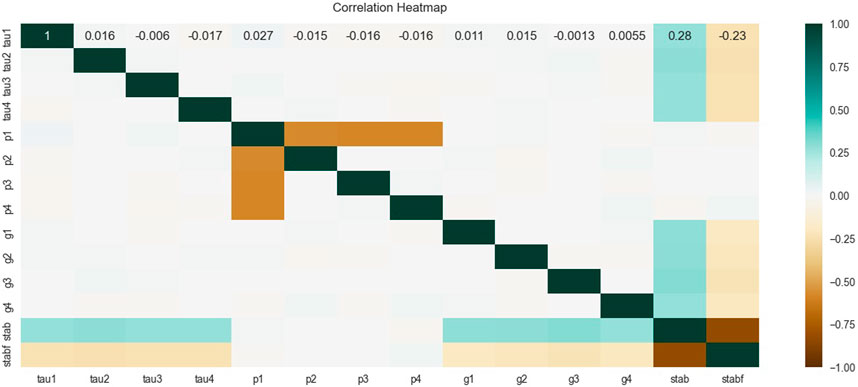
Figure 3. The correlation matrix of the dataset features.

4.2 Data Balancing Evaluation

Figure 4 shows the results of the proposed approach compared to both the standard SMOTE and the GWO-SMOTE, the residual plot of the Guide-waterwheel plant optimization algorithm-optimized SMOTE demonstrates a significant increase in model fit. Through the process of distributing residuals randomly over the horizontal axis, guide-waterwheel plant optimization has successfully reduced the amount of bias in model prediction. A more accurate predictor-response link is demonstrated here, which contributes to an increase in model confidence. Unbiased predictions are displayed on the residual plot of Optimised SMOTE, which also reflects the capacity of the Guide-waterwheel plant optimization algorithm to capture complex data connections successfully. The plot dispersion of the residuals demonstrates the algorithm’s ability to handle intricate patterns and nuances, which in turn makes the model more durable and sophisticated. When compared to standard SMOTE and GWO-SMOTE, homoscedasticity plots for optimized SMOTE, which is based on the use of the Guide-waterwheel plant optimization method, exhibit a substantially lower level of heteroscedasticity. In order to demonstrate the effectiveness of the algorithm in resolving unequal variation, the consistency of the residual variance across predicted values is established. The presence of homoscedasticity enhances the model’s dependability and stability, making it more suitable for producing predictions that are consistent across all of the predictor variables. Furthermore, the improved homoscedasticity of the Guide-waterwheel plant optimization method demonstrates its capacity to distribute defects uniformly.

Figure 4

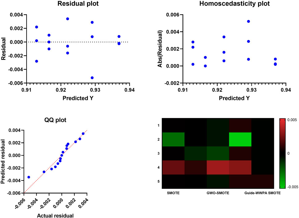
Figure 4. The Residual, homoscedasticity, QQ, and heatmap plots of the prediction results based on the SMOTE approach.

The Guide-waterwheel plant optimization algorithm-optimized SMOTE QQ plot demonstrates considerably better residual normally than both the standard SMOTE and the GWO-SMOTE plots. Based on the fact that the plot points are aligned with the diagonal line, it would suggest that residuals are more usual. The purpose of this normalization is to ensure that the Guide-waterwheel plant optimization approach has rectified any model error deviations from normality, hence confirming the validity of statistical inferences. The accomplishment of the Guide-waterwheel plant optimization method through the construction of a statistically sound model is demonstrated by the QQ plot, which indicates greater normality. The capability of this technique to normalize residuals has the effect of improving statistical tests as well as the assumptions of many statistical studies, which in turn increases the validity of the model. A summary of the performance statistics for the Guide-waterwheel plant optimization algorithm-optimized SMOTE, standard SMOTE, and GWO-SMOTE models is presented in the heatmap graphic. The Guide-waterwheel plant optimization method surpasses SMOTE and GWO-SMOTE in terms of accuracy, precision, recall, and F1-score, as demonstrated by color-coded metrics. The visual representation of the heatmap graphic shows the overall performance of the Guide-waterwheel plant optimization method, hence praising its superiority. The algorithm’s consistent outperformance across a number of criteria provides insight into the existence of a model that is both comprehensive and reliable. If those in charge of making decisions want to have a better understanding of how the algorithm influences the performance of the model, this visualization is beneficial.

With SMOTE, without SMOTE (W/O SMOTE), and with optimized SMOTE in accordance with the Guide-WWPA algorithm (Guide-WWPA SMOTE) are the three preprocessing options that are considered. An accuracy of 90.5% is achieved by beginning with the LSTM model that does not include SMOTE. While the specificity (76%) emphasizes its capacity to minimize false positives, the sensitivity (95.4%), which indicates its potential to identify instances of grid instability efficiently, demonstrates that it is able to do so. The F1 score of 94.2% highlights the model’s balanced performance due to its high level of accuracy. As a result of the influence that oversampling has had on the minority class, the accuracy has increased to 91.3%. An increase in the capacity to recognize unstable grid circumstances is indicated by the sensitivity, which has significantly improved to 96.8%. The model continues to be effective in reducing the number of false positives, as evidenced by the fact that the specificity (77.6%) remains unaffected. The overall improvement in prediction accuracy is confirmed by the fact that the F1 score reaches 95.5% (Table 1).

Table 1

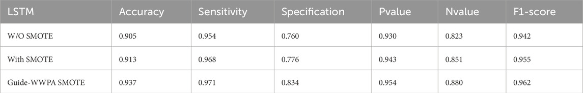
Table 1. Evaluation of the prediction results based on the standard SMOTE, optimized SMOTE and without SMOTE.

In order to prove the efficacy of the Guide-WWPA algorithm in the process of fine-tuning the SMOTE procedure, this configuration achieves a boosted accuracy of 93.7%. The model’s greater ability to identify both stable and unstable grid situations is shown by the fact that both the sensitivity (97.1% of the time) and the specificity (83.4% of the time) indicate improvement. The F1 score achieves an impressive 96.2%, which highlights the influence that the optimized SMOTE has on the achievement of a predictive model that is both well-balanced and very accurate when it comes to prediction. Both the major role that SMOTE plays and the extra benefits that are brought about by the Guide-WWPA algorithm are brought to light by the comparison of the performance of the LSTM model under various preprocessing approaches. For the purpose of achieving improved accuracy, sensitivity, specificity, and overall predictive performance, the optimized SMOTE, which is directed by the Guide-WWPA algorithm, emerges as the most successful preprocessing strategy. In addition to highlighting the potential of improved preprocessing approaches in improving the reliability of predictive models, this illustrates the significance of resolving class imbalance in the context of smart grid stability prediction. When dealing with unbalanced datasets in the context of smart grid stability prediction, researchers and practitioners may make use of these insights to determine how to optimize their method.

ANOVA test results show the importance of the proposed model for smart grid stability prediction under multiple preprocessing methods: without SMOTE, with SMOTE, and with optimized SMOTE using the Guide-WWPA algorithm. ANOVA tables have Treatment, Residual, and Total components. The Treatment component shows how much each preprocessing approach affects model prediction accuracy. The Treatment sum of squares (SS) is 0.00187, with 4 DF and 0.0005 MS. The F-statistic (F (4, 20) = 137.2) shows a significant difference (P < 0.0001) between preprocessing approaches (Table 2). This suggests that at least one preprocessing strategy significantly impacts model prediction. The residual component indicates each preprocessing method’s unexplained variability or mistake. Differences between observed and projected values. With 20 degrees of freedom and an MS of 0.000003, the Residual SS is 0.00007. The Residual component assesses data variability not caused by preprocessing processes, indicating data variability or model inadequacies. The total component shows the model’s predicted performance variability. It combines Treatment and Residual. Total SS is 0.00194, with 24 degrees of freedom. The Total SS shows how much variability pretreatment methods explain relative to data variability. The ANOVA test results indicate that the proposed smart grid stability prediction model performs significantly differently under different preprocessing procedures. The Treatment component, which represents preprocessing procedure variability, greatly affects model performance. These findings emphasize the significance of preprocessing, with the optimized SMOTE employing the Guide-WWPA algorithm possibly improving predictive performance the most. These findings can help researchers and practitioners improve smart grid stability prediction models and preprocessing procedures.

Table 2

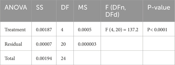
Table 2. Analysis of variance (ANOVA) test applied to the prediction results using the optimized SMOTE approach.

The proposed model for smart grid stability prediction uses several optimization strategies applied to SMOTE, and statistical analysis provides useful insights into performance variances between approaches. Optimization strategies include PSO-SMOTE, GWO-SMOTE, WWPA-SMOTE, and Guide-WWPA SMOTE. Examine and expand each method’s summary data. SMOTE: SMOTE alone is the comparative baseline. The analysis shows a mean accuracy of 0.9129 and a standard deviation of 0.0018 for accuracy values from 0.9101 to 0.9151. The sample mean estimate is precise, with a standard error of 0.0008. PSO-SMOTE, GWO-SMOTE, and WWPA-SMOTE: These optimization approaches make SMOTE accuracy distributions smaller than baseline SMOTE. Each approach improves mean accuracy compared to SMOTE alone; however, range and standard deviation vary, indicating optimization strategy efficacy. The proposed Guide-WWPA SMOTE has the greatest mean accuracy (0.9369) among all approaches, demonstrating its predictive performance improvement. A lower range and standard deviation indicate a more consistent and exact accuracy distribution (Table 3). A deeper statistical summary analysis is possible with the comment extension. Guide-WWPA SMOTE’s shorter range and lower standard deviation indicate stronger predictive performance consistency and stability than other optimization approaches. The reduced standard error of the mean supports this increased precision and provides a more accurate population mean estimate. Comparing percentiles across optimization strategies reveals accuracy distributions. Guide-WWPA SMOTE has greater median and percentile accuracy across the spectrum. Guide-WWPA SMOTE increases the smart grid stability prediction model’s predictive capabilities, yielding more accurate findings than previous optimization approaches. The statistical research shows that Guide-WWPA SMOTE improves smart grid stability prediction model performance. Higher mean accuracy, decreased variability, and increased consistency make it a suitable optimization technique for unbalanced data in smart grid stability prediction tasks. Researchers and practitioners may use these insights to optimize preprocessing and improve the smart grid prediction model’s dependability.

Table 3

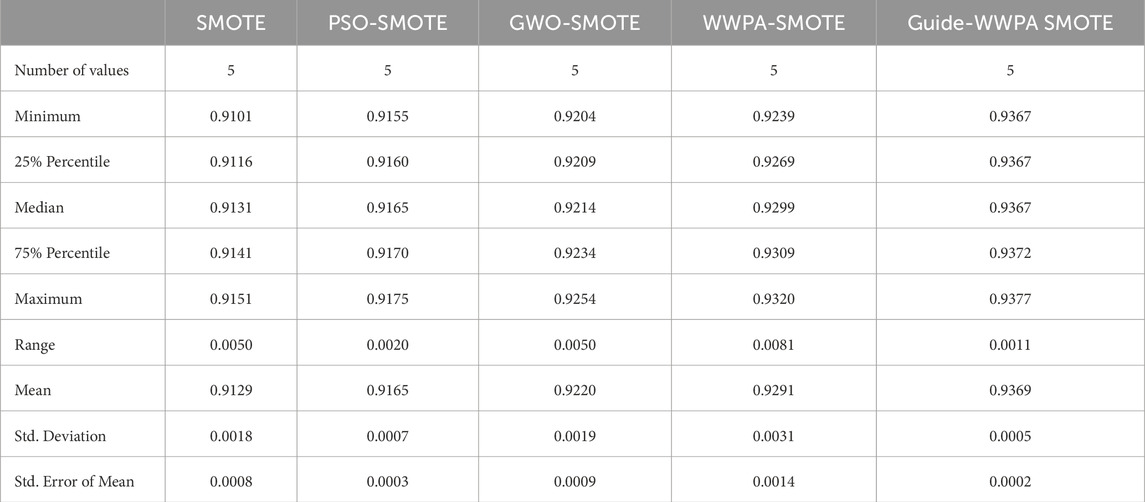
Table 3. Statistical analysis of the data balancing results.

4.3 Evaluating Machine Learning Models

A complete comparison of several algorithms is shown in the findings of the smart grid stability prediction models. The results show that LSTM emerges as the model that is used due to its superior performance. The following metrics will be taken into consideration: accuracy, sensitivity, specificity, Pvalue, Nvalue, and F1-score. Let’s go into the study of each pair of measures. To begin, it exhibits a remarkable accuracy of 81.0%, with a high sensitivity of 89.7%, which indicates that it is proficient in properly recognizing instances of grid stability. This is demonstrated by SVM. On the other hand, the rate of false positives is greater because of the comparatively poor specificity of 62.0%. In situations when accuracy and memory are of the utmost importance, it is essential to strike a balance between sensitivity and specificity. Following that, KNN model gets an accuracy of 82.3% while doing exceptionally well in terms of sensitivity, which is 90.9%. However, in a manner comparable to that of SVM, its specificity is significantly lower, coming in at 72.5%. There is a possibility that KNN has a greater probability of false positives despite the fact that it is quite good at recognizing stable grid conditions. A high level of sensitivity of 91.7% and an accuracy of 83.4% are both features of DT model, which operates well. When it comes to accurately detecting unstable grid states, however, the specificity is still very low at 62.7%, which indicates that there is space for improvement. As we go on to MLP model, we find that it exhibits a high level of sensitivity of 92.0% and an accuracy of 84.3%. A better balance between accurately categorizing stable and unstable circumstances is proposed by the fact that the specificity has improved to 64.8% with this adjustment. In the comparison, the Random Forest (RF) model is one of the models that performs very well since it has an excellent accuracy of 87.4%. It demonstrates its capacity to differentiate between stable and unstable states by virtue of its high sensitivity (93.5%), as well as its high specificity (71.8%). As a result of achieving the maximum accuracy of 89.2%, LSTM model is ultimately selected as the model to be implemented. The sensitivity of this model is 94.4%, which indicates that it is exceedingly capable of identifying grid configurations that are both stable and unstable. Furthermore, the specificity of 76.0 percent reveals a powerful capability to minimize false positives, which makes it more reliable in terms of predicting the stability of smart grids (Table 4). In terms of accuracy, sensitivity, specificity, and overall predictive performance, LSTM model appears to be superior to other algorithms, as demonstrated by the thorough metrics study. This is a promising choice for real-world applications in electrical grid management, which is why LSTM model was chosen as the adopted model. Its greater capacity to reliably anticipate smart grid stability is the reason for this choice.

Table 4

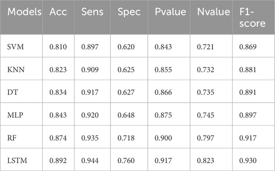
Table 4. Evaluation of various machine learning models.

4.4 Feature Selection Evaluation

The feature selection results from several optimization approaches applied to the smart grid stability dataset show how well different strategies find significant features. Binary bGuide-WWPA, Binary bWWPA, Binary bGWO, Binary bPSO, Binary bBA, Binary bWAO, Binary bBBO, Binary bMVO, Binary bSBO, Binary bFA, and Binary bGA: This measure indicates feature selection accuracy. Lower numbers indicate better performance. The proposed bGuide-WWPA technique has the lowest average error of 0.796, suggesting its efficacy in picking important features (Figures 5, 6). This shows that bGuide-WWPA feature selection is more accurate than other techniques (Table 5). Average Select Size: Each technique selects an average amount of features. Here, bGuide-WWPA has a lower average select size than other approaches, showing it can find a more compact and informative subset of features. This can simplify computation and improve model interpretation. Average Fitness, Best Fitness, Worst Fitness, Std. Fitness: These measures show feature subset quality and variability. With high average fitness, best fitness, and low standard deviation of fitness data, bGuide-WWPA performs well. This indicates that bGuide-WWPA’s feature subsets are accurate, consistent, and robust. The proposed bGuide-WWPA successfully selects key features for smart grid stability prediction. Its decreased average error, small subset of features, and high fitness values make it preferable to other feature selection approaches. These findings can help researchers and practitioners enhance smart grid management forecasting models and feature selection.

Figure 5

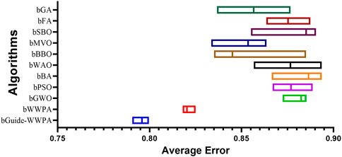
Figure 5. The average error of the prediction results based on the feature selection methods.

Figure 6

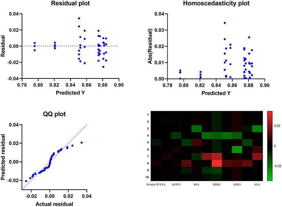
Figure 6. Analysis Plots of the feature selection results.

Table 5

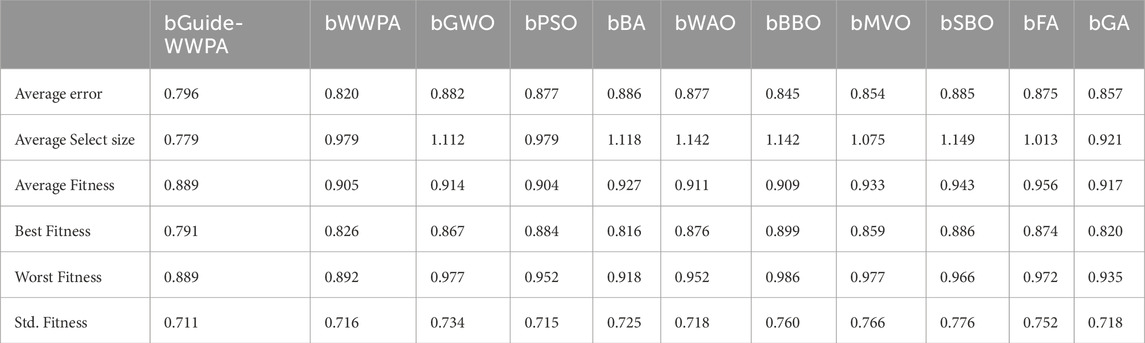
Table 5. Evaluation of the feature selection results.

ANOVA test on smart grid stability prediction feature selection results using bGuide-WWPA, bWWPA, bGWO, bPSO, bBA, bWAO, bBBO, bMVO, bSBO, bFA, and bGA shows how these methods affect predictive performance. Treatment: The Treatment component indicates how much each feature selection approach affects predicted accuracy. The Treatment SS is 0.080, with 10 DF and 0.008008 MS. The F-statistic (F (10, 99) = 115.4) shows a significant difference (P < 0.0001) across feature selection approaches (Table 6). This suggests that at least one feature selection approach significantly affects model prediction. Residual: Each feature selection method’s unexplained variability or inaccuracy is the residual component. Differences between observed and projected values are included. With 99 degrees of freedom and an MS of 0.00006942, the Residual SS is 0.007. The Residual component assesses data variability not caused by feature selection techniques, indicating data variability or model shortcomings. Total: The Total component indicates model prediction performance variability. It combines Treatment and Residual. The Total SS is 0.087 with 109 degrees of freedom. The Total SS shows how much variability feature selection strategies explain relative to data variability. The ANOVA test findings indicate that smart grid stability prediction feature selection approaches function differently. The Treatment component, which reflects feature selection process variability, is critical to model performance. These findings emphasize the relevance of feature selection, which may improve smart grid management prediction model accuracy and dependability. These findings can help researchers and practitioners improve smart grid stability prediction predictive models and feature selection procedures.

Table 6

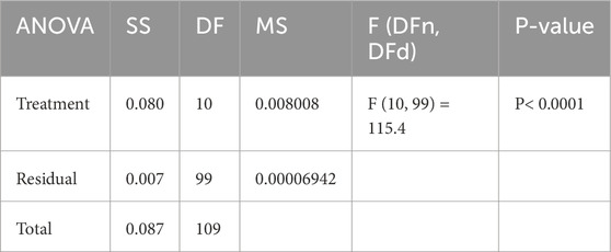
Table 6. ANOVA test applied to the feature selection results.

The Wilcoxon signed-rank test helps determine the relevance of smart grid stability prediction technique differences between matched feature selection approaches. The medians of the differences between the paired feature selection approaches are compared to a theoretical median of zero. Examine and expand on the important results. Theoretical and Actual Medians: The theoretical median is zero, suggesting no predicted difference between the paired feature selection approaches. Actual median values show method discrepancies. The median for bGuide-WWPA is 0.796, bWWPA is 0.820, etc. These values indicate the main procedure differences. Each feature selection technique is matched with the others, creating 10 pairings. The absolute differences between paired feature selection approaches are summed according to signed rankings. All pairings have 55 signed rankings, indicating consistency in ranking discrepancies across approaches. The sum of positive rankings reflects ranks given to positive differences (where the first technique has a higher median than the second). In contrast, the total of negative ranks represents ranks assigned to negative differences. All differences are positive in this test; thus, positive and negative ranks are equal. Two-Tailed P-Value: The P number reflects the chance of seeing the findings (or more extreme) under the null hypothesis of no difference between the matched feature selection procedures. For all couples, the P value is 0.002, strongly rejecting the null hypothesis (Table 7). This suggests that feature selection approaches varied greatly. The discrepancy column shows variations between the matched feature selection approaches. These medians reveal technique differences in direction and size. The Wilcoxon signed-rank test shows substantial differences amongst smart grid stability prediction paired feature selection approaches. Choosing the right feature selection approach is important since the constant sum of signed rankings and low P values indicate strong findings across all pairings. These findings can help researchers and practitioners choose the best feature selection method for smart grid stability prediction.

Table 7

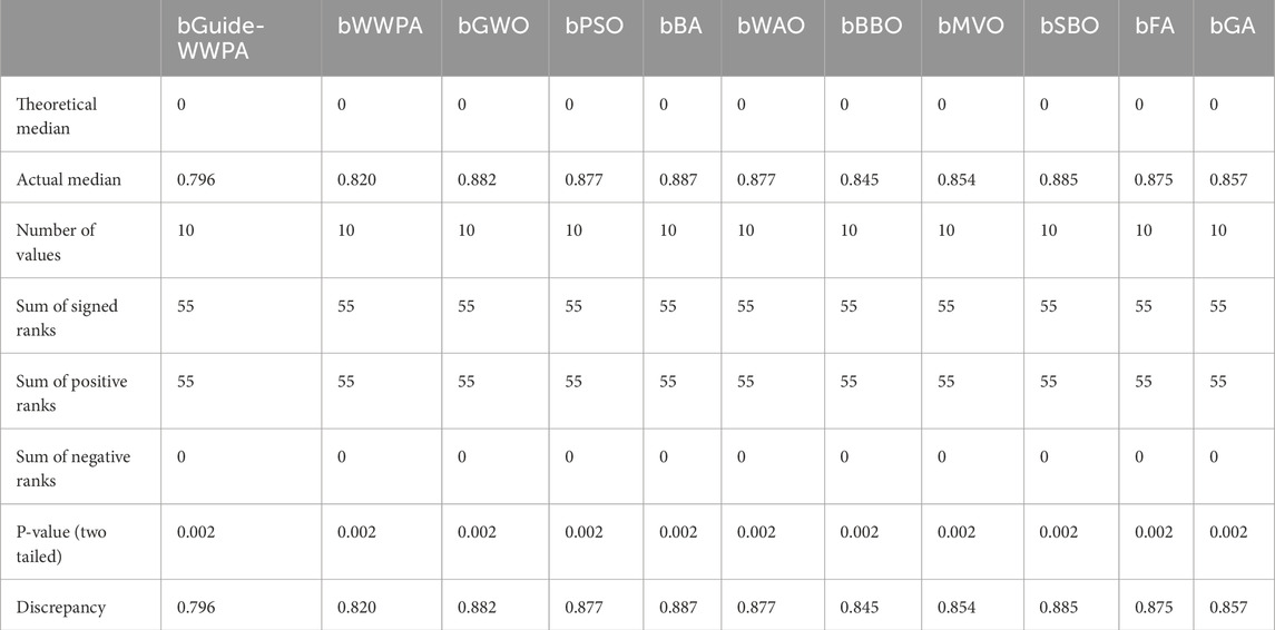
Table 7. Wilcoxon signed rank test applied to the feature selection results.

4.5 Smart Grid Stability Prediction Evaluation

When compared to earlier methods of feature selection, the Smart Grid Stability Prediction that makes use of the optimized Guide-WWPA + LSTM model distinguishes itself by displaying the prediction performance of the model. It has been demonstrated that Guide-WWPA + LSTM is more accurate than other LSTM models such as PSO + LSTM, GA + LSTM, GWO + LSTM, MVO + LSTM, BBO + LSTM, WOA + LSTM, and the standard LSTM model. A more concentrated and smaller accuracy distribution in the histogram is indicative of predictive performance that is of a higher quality. In order to increase the accuracy of smart grid stability forecasts, Guide-WWPA is able to detect significant factors that optimize the LSTM model. In terms of accuracy and prediction error variance, the accuracy histogram demonstrates that the Guide-WWPA + LSTM model works better than other feature selection techniques. With the enhanced Guide-WWPA method, the model’s capacity to generalize to new data is improved, resulting in more consistent and predictable performance (Figures 7–9). This is accomplished by effectively traversing across feature space and detecting variables that have significance. When it comes to smart grids, having credible stability forecasts is necessary for ensuring the safety and effectiveness of the network. The Guide-WWPA provides a higher level of accuracy when compared to other classification methods such as PSO + LSTM, GA + LSTM, GWO + LSTM, MVO + LSTM, BBO + LSTM, WOA + LSTM, and the standard LSTM.

Figure 7

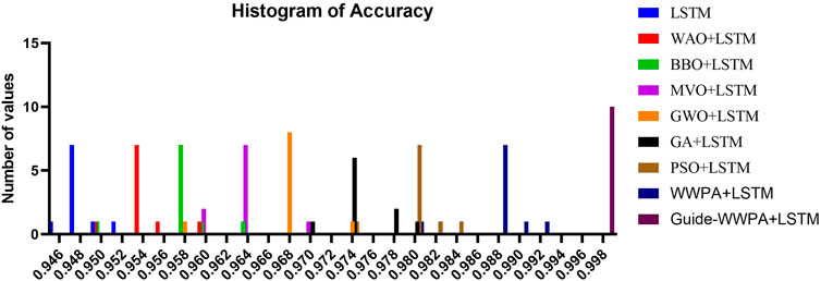
Figure 7. The histogram of the prediction accuracy.

Figure 8

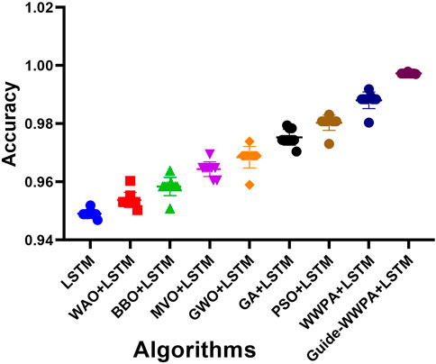
Figure 8. The accuracy of the prediction results achieved by various prediction algorithms.

Figure 9

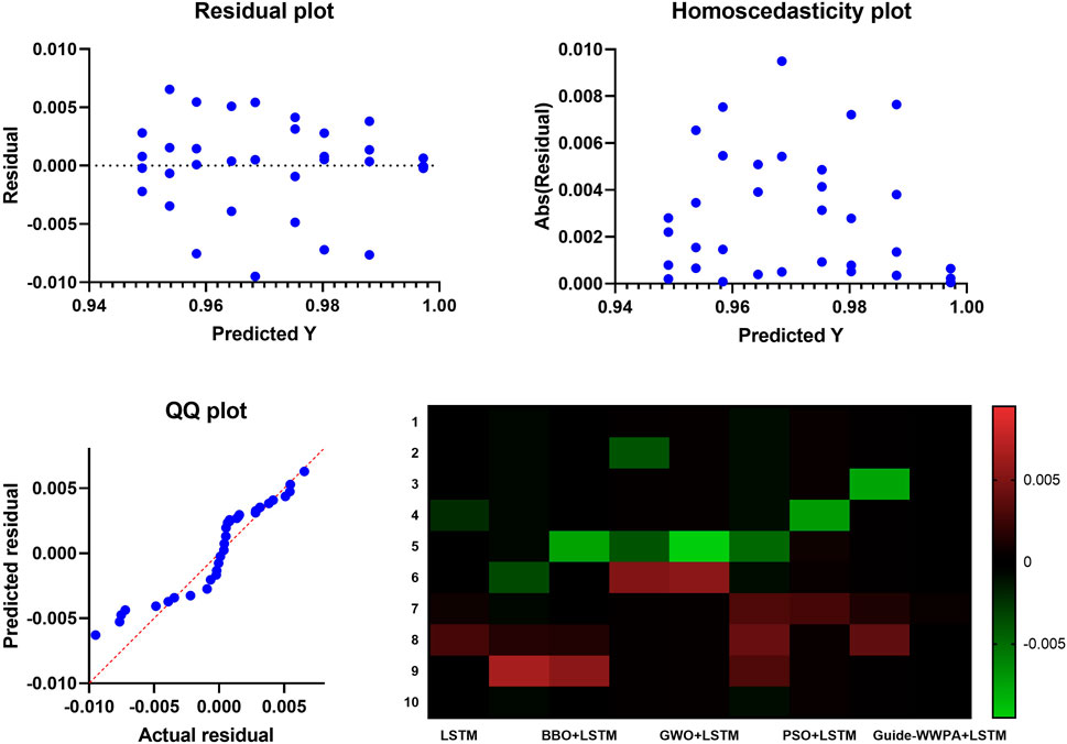
Figure 9. Analysis plots of results of the smart grid stability prediction.

The capability of the algorithm to recognize important features and effectively collaborate with the LSTM model contributes to an increase in the predictive capacity of the hybrid model. The Guide-WWPA + LSTM model may perform better than other techniques if it is essential to have intelligent grid stability forecasts that are precise and reliable. Other feature selection methods are outperformed by the Smart Grid Stability Prediction accuracy histogram, which makes use of the improved Guide-WWPA + LSTM model. A demonstration of the LSTM model’s expanded predictive capacity is provided by Guide-WWPA’s enhanced and consistent accuracy distribution as well as its reduced prediction errors. Under real-world applications, this hybrid technique for predicting the stability of smart grids appears to have a lot of potential. It may even surpass other feature selection methods that are now under implementation.

When comparing the Guide-WWPA + LSTM model to the WWPA + LSTM model for the purpose of predicting the stability of smart grids, the ROC curve is an essential visual tool, as depicted in Figure 10. In order to demonstrate that the models are able to differentiate between stable and unstable circumstances, the ROC curve illustrates the compromise that exists between the true positive rate and the false positive rate. By having a greater area under the curve (AUC), which indicates better discrimination and prediction, the recommended Guide-WWPA + LSTM model surpasses the WWPA + LSTM model in this comparison. In the Guide-WWPA + LSTM model, the ROC curve gets steeper and more convex as it is studied more carefully. This indicates that the model has greater sensitivity and specificity across all classification thresholds. With the help of the Guide-WWPA algorithm, the feature selection process was optimized, which in turn enabled the LSTM model to generate predictions that were precise and reliable. For the purpose of managing energy proactively and efficiently, achieving smart grid stability prediction requires an expanded discriminating power to recognize prospective instability occurrences. In addition to that, the comment investigates the use of ROC curve comparison in the real world. It is possible that the Guide-WWPA + LSTM model, which has superior performance, would lower the number of false positives and negatives that are associated with smart grid stability prediction. This will reduce the risk of ineffective actions or the occurrence of key instability events. By ensuring the dependability and robustness of smart grids this makes it easier to make decisions on the management of electrical networks. With regard to discriminatory power and predictive performance, the Guide-WWPA + LSTM model is superior to the WWPA + LSTM model. This conclusion is based on the results of ROC curve analysis conducted on the findings of smart grid stability prediction. In order to improve the accuracy and dependability of the LSTM model, the Guide-WWPA approach optimizes the selection of features. Exact stability projections are necessary for smart grid operations in order to guarantee the long-term reliability and effectiveness of the electrical framework. Using the Guide-WWPA + LSTM model for smart grid stability prediction, energy management and grid reliability may both be improved over time.

Figure 10

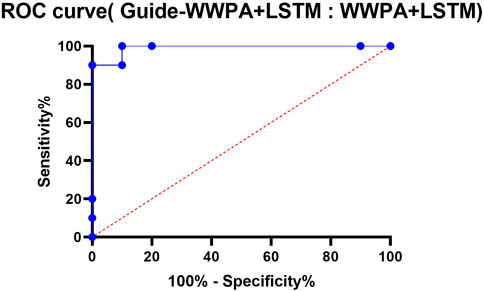
Figure 10. The ROC cCurve between Guide-WWPA + LSTM and WWPA + LSTM.

Both Guide-WWPA + LSTM and WWPA+LSTM models have AUCs of 0.99, which is high. This suggests that Guide-WWPA + LSTM and WWPA + LSTM models may accurately categorize cases due to their strong discriminatory strength. Standard Error: Measures AUC estimate variability or precision. We have a tiny standard error of 0.01616 around the AUC estimate. 95% Confidence Interval: The 95% confidence interval gives us a reasonable estimate of the real AUC value. The CI is 0.9583–1.000, showing good AUC estimate confidence. A P-value reflects the statistical significance of the performance difference between the two models. The P-value is 0.0002, below the significance level of 0.05. This shows that Guide-WWPA + LSTM outperforms WWPA + LSTM statistically. Data: The data summary lists the number of controls (LSTM model-classified as normal stability) and patients (LSTM-classified as unstable) utilized in the analysis. Both models were tested with 10 controls and 10 patients, and no data was missing. The ROC curve shows that Guide-WWPA + LSTM and WWPA + LSTM models predict smart grid stability effectively. Guide-WWPA + LSTM may have a modest performance advantage over WWPA + LSTM, as seen by the low P-value. For reliable smart grid stability prediction, optimization methods such as Guide-WWPA and LSTM models work well (Table 8).

Table 8

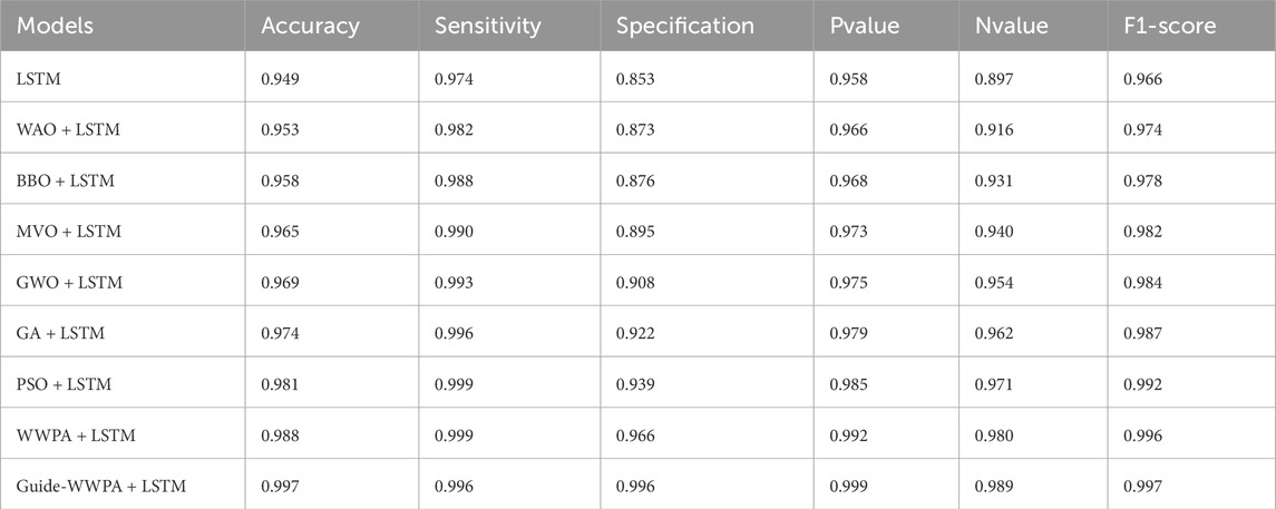
Table 8. Prediction results based on various optimization methods.

The ANOVA test findings, in Table 9, show that smart grid stability prediction approaches function differently. The treatment component shows significant variability between prediction approaches, with an SS of 0.02069 and a high F-statistic of 383.6 (with 8 and 81 degrees of freedom), resulting in a low P-value (<0.0001). This shows that at least one prediction approach significantly affects model prediction. An SS of 0.000546 and an MS of 0.000006741 indicate a tiny residual component, which accounts for unexplained variability or error in each prediction technique. This suggests that predicted performance variability is mostly due to technique variations rather than random variability within each method. A total SS of 0.02123 (89 degrees of freedom) shows model prediction performance variability. The large ANOVA difference emphasizes the importance of choosing the right prediction approach, which may improve the accuracy and dependability of smart grid stability prediction models.

Table 9

Table 9. ANOVA test results of the prediction results.

The Wilcoxon signed-rank test shows that Guide-WWPA + LSTM outperforms alternative smart grid stability prediction approaches as presented in Table 10. The theoretical median for all approaches is zero, showing no performance difference from Guide-WWPA + LSTM. However, each method’s median results, ranging from 0.949 to 0.997, show significant performance differences from Guide-WWPA + LSTM. The sum of signed rankings appears to rank performance differences consistently across all approaches, supporting this disagreement. Each technique performs significantly better than Guide-WWPA + LSTM (P-value 0.002, two-tailed). This strongly contradicts the null hypothesis that Guide-WWPA + LSTM performs similarly to the other approaches. The Wilcoxon signed-rank test findings show that Guide-WWPA + LSTM outperforms alternative smart grid stability prediction approaches. This emphasizes the significance of choosing the best approach, with Guide-WWPA + LSTM performing best.

Table 10

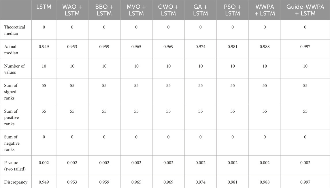
Table 10. Wilcoxon signed rank test applied to the prediction results.

The statistical test of smart grid stability prediction using LSTM, WAO + LSTM, BBO + LSTM, MVO + LSTM, GWO + LSTM, GA + LSTM, PSO + LSTM, WWPA + LSTM, and Guide-WWPA + LSTM shows their performance and variability. Analysis of the statistics reveals each method’s predictive power as presented in Table 11. Central tendency measurements like the mean, median, and quartiles help us comprehend each method’s usual performance. Guide-WWPA + LSTM has a mean smart grid stability prediction accuracy of 0.997. Range and standard deviation show predicted performance metrics’ distribution around the mean. A lower range and standard deviation indicate less performance variability across experiments or observations. Guide-WWPA + LSTM has the lowest standard deviation of 0.000, showing consistent performance across assessments. Mean confidence intervals also show the accuracy of estimated performance levels. Guide-WWPA + LSTM ’ s narrow confidence intervals suggest strong mean performance value confidence. Skewness and kurtosis assess performance value distribution shape. The distribution is skewed to the right for positive skewness, suggesting lower performance values, and to the left for negative skewness, indicating greater performance values. Kurtosis indicates distribution peaking. Understanding these measurements helps evaluate each method’s performance value distribution. By revealing the performance characteristics of the tested approaches, statistical analysis allows stakeholders to choose them for smart grid stability prediction.

Table 11

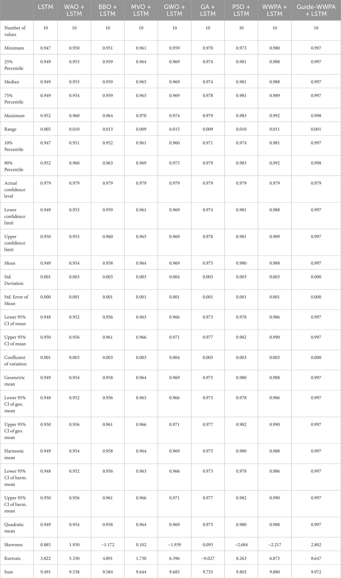
Table 11. Statistical analysis of the prediction results.

5 Conclusion

This paper proposed a novel Guide-WWPA+LSTM model for boosting the prediction accuracy of smart grid stability. On the smart grid dataset that is available from the UCI Machine Learning Repository, the proposed model is demonstrated through experimentation. The effectiveness of Guide-WWPA+LSTM is evaluated in comparison to that of various optimization methods and conventional machine learning models such as LSTM, SVM, DT, and MLP. Regarding accuracy, precision, loss, and ROC curve metrics, the comparison study demonstrates that the proposed model is superior to the other models. In comparison to other conventional models, the proposed model attained an accuracy of 99.7%. In addition, the proposed model has a sensitivity, specificity, Pvalue, Nvalue and F1-score as 97.6%, 99.6%, 99.9% and 99.7%. The ROC curve is another indicator that demonstrates how successful the proposed model should be. The model that was presented accomplishes an ROC of 99.00%, which is superior to the performance of the other models. It is possible to implement a context-aware model as part of the work that will be done in the future in order to meet the ever-changing demands for electricity and enhance the dependability of smart grids.

Data availability statement

The original contributions presented in the study are included in the article/Supplementary Material, further inquiries can be directed to the corresponding authors.

Author contributions

KF: Writing–original draft, Writing–review & editing. DK: Writing–original draft, Writing–review & editing. E-SE-k: Writing–original draft, Writing–review & editing. Marwa Eid: Writing–original draft, Writing–review & editing. Abdelhameed Ibrahim: Writing–original draft, Writing–review & editing. LA: Writing–original draft, Writing–review & editing. Nima Khodadadi: Writing–original draft, Writing–review & editing. Abdelaziz Abdelhamid: Writing–original draft, Writing–review & editing.

Funding

The author(s) declare that no financial support was received for the research, authorship, and/or publication of this article.

Acknowledgments

Princess Nourah bint Abdulrahman University Researchers Supporting Project number (PNURSP2024R 300), Princess Nourah bint Abdulrahman University, Riyadh, Saudi Arabia.

Conflict of interest

The authors declare that the research was conducted in the absence of any commercial or financial relationships that could be construed as a potential conflict of interest.

Publisher’s note

All claims expressed in this article are solely those of the authors and do not necessarily represent those of their affiliated organizations, or those of the publisher, the editors and the reviewers. Any product that may be evaluated in this article, or claim that may be made by its manufacturer, is not guaranteed or endorsed by the publisher.

References

Abdelhamid, A. A., Towfek, S. K., Khodadadi, N., Alhussan, A. A., Khafaga, D. S., Eid, M. M., et al. (2023). Waterwheel plant algorithm: a novel metaheuristic optimization method. Processes 11, 1502. doi:10.3390/pr11051502

CrossRef Full Text | Google Scholar

Adil, M., Javaid, N., Qasim, U., Ullah, I., Shafiq, M., and Choi, J. G. (2020). LSTM and bat-based RUSBoost approach for electricity theft detection. Appl. Sci. 10, 4378. doi:10.3390/app10124378

CrossRef Full Text | Google Scholar

Ahmed, S., Lee, Y., Hyun, S. H., and Koo, I. (2019). Unsupervised machine learning-based detection of covert data integrity assault in smart grid networks utilizing isolation forest. IEEE Trans. Inf. Forensics Secur. 14, 2765–2777. doi:10.1109/TIFS.2019.2902822

CrossRef Full Text | Google Scholar

Alazab, M., Khan, S., Krishnan, S. S. R., Pham, Q. V., Reddy, M. P. K., and Gadekallu, T. R. (2020). A multidirectional LSTM model for predicting the stability of a smart grid. IEEE Access 8, 85454–85463. doi:10.1109/ACCESS.2020.2991067

CrossRef Full Text | Google Scholar

M. Alazab, and M. Tang (2019). Deep learning Applications for cyber security. Advanced sciences and technologies for security applications (Cham: Springer International Publishing). doi:10.1007/978-3-030-13057-2

CrossRef Full Text | Google Scholar

Almalaq, A., and Edwards, G. (2017). “A review of deep learning methods applied on load forecasting,” in USA, 18-21 Dec. 2017, 511–516. doi:10.1109/ICMLA.2017.0-110

CrossRef Full Text | Google Scholar

Almetwally, E. M., and Meraou, M. (2022). Application of environmental data with new extension of nadarajah-haghighi distribution. Comput. J. Math. Stat. Sci. 1, 26–41. doi:10.21608/cjmss.2022.271186

CrossRef Full Text | Google Scholar

J. L. Awange, P. Swarm Optimization, J. L. Awange, B. Paláncz, R. H. Lewis, and L. Völgyesi (2018). Mathematical geosciences: hybrid symbolic-numeric methods (Cham: Springer International Publishing), 167–184. doi:10.1007/978-3-319-67371-4_6

CrossRef Full Text | Google Scholar

Bajaj, M., and Singh, A. K. (2020). Grid integrated renewable DG systems: a review of power quality challenges and state-of-the-art mitigation techniques. Int. J. Energy Res. 44, 26–69. doi:10.1002/er.4847

CrossRef Full Text | Google Scholar

Bassamzadeh, N., and Ghanem, R. (2017). Multiscale stochastic prediction of electricity demand in smart grids using Bayesian networks. Appl. Energy 193, 369–380. doi:10.1016/j.apenergy.2017.01.017

CrossRef Full Text | Google Scholar

Chawla, N. V., Bowyer, K. W., Hall, L. O., and Kegelmeyer, W. P. (2002). SMOTE: synthetic minority over-sampling technique. J. Artif. Intell. Res. 16, 321–357. doi:10.1613/jair.953

CrossRef Full Text | Google Scholar

Chen, K. (2019). Indirect PCA dimensionality reduction based machine learning algorithms for power system transient stability assessment. 2019 IEEE Innov. Smart Grid Technol. - Asia (ISGT Asia) (Chengdu, China IEEE), 4175–4179. doi:10.1109/ISGT-Asia.2019.8881370

CrossRef Full Text | Google Scholar

Din, I. U., Guizani, M., Rodrigues, J. J., Hassan, S., and Korotaev, V. V. (2019). Machine learning in the Internet of Things: designed techniques for smart cities. Future Gener. Comput. Syst. 100, 826–843. doi:10.1016/j.future.2019.04.017

CrossRef Full Text | Google Scholar

Fister, I., Fister, I., Yang, X. S., and Brest, J. (2013). A comprehensive review of firefly algorithms. Swarm Evol. Comput. 13, 34–46. doi:10.1016/j.swevo.2013.06.001

CrossRef Full Text | Google Scholar

Ghorbanian, M., Dolatabadi, S. H., and Siano, P. (2019). Big data issues in smart grids: a survey. IEEE Syst. J. 13, 4158–4168. doi:10.1109/JSYST.2019.2931879

CrossRef Full Text | Google Scholar

Hafeez, G., Alimgeer, K. S., and Khan, I. (2020a). Electric load forecasting based on deep learning and optimized by heuristic algorithm in smart grid. Appl. Energy 269, 114915. doi:10.1016/j.apenergy.2020.114915

CrossRef Full Text | Google Scholar

Hafeez, G., Alimgeer, K. S., Qazi, A. B., Khan, I., Usman, M., Khan, F. A., et al. (2020b). A hybrid approach for energy consumption forecasting with a new feature engineering and optimization framework in smart grid. IEEE Access 8, 96210–96226. doi:10.1109/ACCESS.2020.2985732

CrossRef Full Text | Google Scholar

Hafeez, G., Alimgeer, K. S., Wadud, Z., Shafiq, Z., Ali Khan, M. U., Khan, I., et al. (2020c). A novel accurate and fast converging deep learning-based model for electrical energy consumption forecasting in a smart grid. Energies 13, 2244. doi:10.3390/en13092244

CrossRef Full Text | Google Scholar

Hafeez, G., Javaid, N., Riaz, M., Ali, A., Umar, K., and Iqbal, Z. (2020d). “Day ahead electric load forecasting by an intelligent hybrid model based on deep learning for smart grid,” in Complex, intelligent, and software intensive systems. Editors L. Barolli, F. K. Hussain, and M. Ikeda (Cham: Springer International Publishing), 993, 36–49. doi:10.1007/978-3-030-22354-0_4

CrossRef Full Text | Google Scholar

Hafeez, G., Khan, I., Jan, S., Shah, I. A., Khan, F. A., and Derhab, A. (2021). A novel hybrid load forecasting framework with intelligent feature engineering and optimization algorithm in smart grid. Appl. Energy 299, 117178. doi:10.1016/j.apenergy.2021.117178

CrossRef Full Text | Google Scholar

Hong, Y., Zhou, Y., Li, Q., Xu, W., and Zheng, X. (2020). A deep learning method for short-term residential load forecasting in smart grid. IEEE Access 8, 55785–55797. doi:10.1109/ACCESS.2020.2981817

CrossRef Full Text | Google Scholar

Immanuel, S. D., and Chakraborty, U. K. (2019). “Genetic algorithm: an approach on optimization,” in 2019 International Conference on Communication and Electronics Systems (ICCES), China, 17-19 July 2019, 701–708. doi:10.1109/ICCES45898.2019.9002372

CrossRef Full Text | Google Scholar

Irshad, O., Khan, M. U. G., Iqbal, R., Basheer, S., and Bashir, A. K. (2020). Performance optimization of IoT based biological systems using deep learning. Comput. Commun. 155, 24–31. doi:10.1016/j.comcom.2020.02.059

CrossRef Full Text | Google Scholar

Iwendi, C., Khan, S., Anajemba, J. H., Bashir, A. K., and Noor, F. (2020). Realizing an efficient IoMT-assisted patient diet recommendation system through machine learning model. IEEE Access 8, 28462–28474. doi:10.1109/ACCESS.2020.2968537

CrossRef Full Text | Google Scholar

Iwendi, C., Maddikunta, P. K. R., Gadekallu, T. R., Lakshmanna, K., Bashir, A. K., and Piran, M. J. (2021). A metaheuristic optimization approach for energy efficiency in the IoT networks. Softw. Pract. Exp. 51, 2558–2571. doi:10.1002/spe.2797

CrossRef Full Text | Google Scholar

Jin, L., Fuggle, A., Roberts, H., and Armstrong, C. P. (2023). Using machine learning to predict shear wave velocity. Geo-congress 2023. Los Angeles, California: American Society of Civil Engineers, 142–152. doi:10.1061/9780784484678.015

CrossRef Full Text | Google Scholar

Jindal, A., Dua, A., Kaur, K., Singh, M., Kumar, N., and Mishra, S. (2016). Decision tree and SVM-based data analytics for theft detection in smart grid. IEEE Trans. Industrial Inf. 12, 1005–1016. doi:10.1109/TII.2016.2543145

CrossRef Full Text | Google Scholar

Kotb, Y., Al Ridhawi, I., Aloqaily, M., Baker, T., Jararweh, Y., and Tawfik, H. (2019). Cloud-based multi-agent cooperation for IoT devices using workflow-nets. J. Grid Comput. 17, 625–650. doi:10.1007/s10723-019-09485-z

CrossRef Full Text | Google Scholar

Kumar, N., Zeadally, S., and Rodrigues, J. J. (2016). Vehicular delay-tolerant networks for smart grid data management using mobile edge computing. IEEE Commun. Mag. 54, 60–66. doi:10.1109/MCOM.2016.7588230

CrossRef Full Text | Google Scholar

Kumar, S., K, Y. H., Kumar Sharma, N., Bajaj, M., Naithani, D., and Maindola, M. (2022). “Classical secondary control techniques in microgrid systems – a review,” in 2022 2nd International Conference on Innovative Sustainable Computational Technologies (CISCT), China, 23-24 Dec. 2022, 1–6. doi:10.1109/CISCT55310.2022.10046557

CrossRef Full Text | Google Scholar

Liu, Y., Jiang, Y., Zhang, X., Pan, Y., and Wang, J. (2023). An improved grey wolf optimizer algorithm for identification and location of gas emission. J. Loss Prev. Process Industries 82, 105003. doi:10.1016/j.jlp.2023.105003

CrossRef Full Text | Google Scholar

Mahmud, K., Sahoo, A. K., Fernandez, E., Sanjeevikumar, P., and Holm-Nielsen, J. B. (2020). Computational tools for modeling and analysis of power generation and transmission systems of the smart grid. IEEE Syst. J. 14, 3641–3652. doi:10.1109/JSYST.2020.2964436

CrossRef Full Text | Google Scholar

Martínez-Rodríguez, D., Novella, R., Bracho, G., Gomez-Soriano, J., Fernandes, C., Lucchini, T., et al. (2023). A particle swarm optimization algorithm with novelty search for combustion systems with ultra-low emissions and minimum fuel consumption. Appl. Soft Comput. 143, 110401. doi:10.1016/j.asoc.2023.110401

CrossRef Full Text | Google Scholar

Mirjalili, S., and Lewis, A. (2016). The whale optimization algorithm. Adv. Eng. Softw. 95, 51–67. doi:10.1016/j.advengsoft.2016.01.008

CrossRef Full Text | Google Scholar

Mirjalili, S., Mirjalili, S. M., and Hatamlou, A. (2016). Multi-verse optimizer: a nature-inspired algorithm for global optimization. Neural Comput. Appl. 27, 495–513. doi:10.1007/s00521-015-1870-7

CrossRef Full Text | Google Scholar

Mirjalili, S., Mirjalili, S. M., and Lewis, A. (2014). Grey wolf optimizer. Adv. Eng. Softw. 69, 46–61. doi:10.1016/j.advengsoft.2013.12.007

CrossRef Full Text | Google Scholar

Moldovan, D., and Salomie, I. (2019). “Detection of sources of instability in smart grids using machine learning techniques,” in 2019 IEEE 15th International Conference on Intelligent Computer Communication and Processing (ICCP), Cluj-Napoca, Romania, 5-7 Sept. 2019 (IEEE), 175–182. doi:10.1109/ICCP48234.2019.8959649

CrossRef Full Text | Google Scholar

Muhammed, H. Z., and Almetwally, E. (2024). Bayesian and non-bayesian estimation for the shape parameters of new versions of bivariate inverse weibull distribution based on progressive type II censoring. Comput. J. Math. Stat. Sci. 3, 85–111. doi:10.21608/cjmss.2023.250678.1028

CrossRef Full Text | Google Scholar

Nawaz, A., Hafeez, G., Khan, I., Jan, K. U., Li, H., Khan, S. A., et al. (2020). An intelligent integrated approach for efficient demand side management with forecaster and advanced metering infrastructure frameworks in smart grid. IEEE Access 8, 132551–132581. doi:10.1109/ACCESS.2020.3007095

CrossRef Full Text | Google Scholar

Panda, S., Mohanty, S., Rout, P. K., Sahu, B. K., Bajaj, M., Zawbaa, H. M., et al. (2022). Residential Demand Side Management model, optimization and future perspective: a review. Energy Rep. 8, 3727–3766. doi:10.1016/j.egyr.2022.02.300

CrossRef Full Text | Google Scholar

Pham, Q. V., Fang, F., Ha, V. N., Piran, M. J., Le, M., Le, L. B., et al. (2020). A survey of multi-access edge computing in 5G and beyond: fundamentals, technology integration, and state-of-the-art. IEEE Access 8, 116974–117017. doi:10.1109/ACCESS.2020.3001277

CrossRef Full Text | Google Scholar

Razavi, R., Gharipour, A., Fleury, M., and Akpan, I. J. (2019). A practical feature-engineering framework for electricity theft detection in smart grids. Appl. Energy 238, 481–494. doi:10.1016/j.apenergy.2019.01.076

CrossRef Full Text | Google Scholar

Reddy, G. T., Reddy, M. P. K., Lakshmanna, K., Kaluri, R., Rajput, D. S., Srivastava, G., et al. (2020). Analysis of dimensionality reduction techniques on big data. IEEE Access 8, 54776–54788. doi:10.1109/ACCESS.2020.2980942

CrossRef Full Text | Google Scholar

Samareh Moosavi, S. H., and Khatibi Bardsiri, V. (2017). Satin bowerbird optimizer: a new optimization algorithm to optimize anfis for software development effort estimation. Eng. Appl. Artif. Intell. 60, 1–15. doi:10.1016/j.engappai.2017.01.006

CrossRef Full Text | Google Scholar

Shafiq, M., Yu, X., Bashir, A. K., Chaudhry, H. N., and Wang, D. (2018). A machine learning approach for feature selection traffic classification using security analysis. J. Supercomput. 74, 4867–4892. doi:10.1007/s11227-018-2263-3

CrossRef Full Text | Google Scholar

Shrivastava, P., and Yadav, R. (2023). Deep learning approach for intelligent intrusion detection system. SSRN Electron. J. doi:10.2139/ssrn.4386519

CrossRef Full Text | Google Scholar

Siddiqui, I. F., Lee, S. U. J., Abbas, A., and Bashir, A. K. (2017). Optimizing lifespan and energy consumption by smart meters in green-cloud-based smart grids. IEEE Access 5, 20934–20945. doi:10.1109/ACCESS.2017.2752242

CrossRef Full Text | Google Scholar

Sutskever, I., Vinyals, O., and Le, Q. V. Sequence to sequence learning with neural networks (2014). doi:10.48550/arXiv.1409.3215

CrossRef Full Text | Google Scholar

Syed, D., Refaat, S. S., and Abu-Rub, H. (2020). Performance evaluation of distributed machine learning for load forecasting in smart grids. Cybern. Inf. (K&I) (Velke Karlovice, Czech Repub. IEEE) 2020, 1–6. doi:10.1109/KI48306.2020.9039797

CrossRef Full Text | Google Scholar

Szegedy, C., Liu, W., Jia, Y., Sermanet, P., Reed, S., Anguelov, D., et al. Going deeper with convolutions (2014). doi:10.48550/arXiv.1409.4842

CrossRef Full Text | Google Scholar

Vinayakumar, R., Alazab, M., Soman, K. P., Poornachandran, P., and Venkatraman, S. (2019). Robust intelligent malware detection using deep learning. IEEE Access 7, 46717–46738. doi:10.1109/ACCESS.2019.2906934

CrossRef Full Text | Google Scholar

Wood, D. A. (2020). Predicting stability of a decentralized power grid linking electricity price formulation to grid frequency applying an optimized data-matching learning network to simulated data. Technol. Econ. Smart Grids Sustain. Energy 5, 3. doi:10.1007/s40866-019-0074-0

CrossRef Full Text | Google Scholar

Xiang, H., Zou, Q., Nawaz, M. A., Huang, X., Zhang, F., and Yu, H. (2023). Deep learning for image inpainting: a survey. Pattern Recognit. 134, 109046. doi:10.1016/j.patcog.2022.109046

CrossRef Full Text | Google Scholar

Yu, D., and Deng, L. (2015). Automatic speech recognition: a deep learning approach. Signals and communication technology. London: Springer. doi:10.1007/978-1-4471-5779-3

CrossRef Full Text | Google Scholar

Zhang, D., Han, X., and Deng, C. (2018). Review on the research and practice of deep learning and reinforcement learning in smart grids. CSEE J. Power Energy Syst. 4, 362–370. doi:10.17775/CSEEJPES.2018.00520

CrossRef Full Text | Google Scholar

Nomenclature