 Yiyi Le1
 Jing Wen
94% of researchers rate our articles as excellent or good
Learn more about the work of our research integrity team to safeguard the quality of each article we publish.
Find out more
ORIGINAL RESEARCH article
Front. Energy Res. , 13 June 2024
Sec. Carbon Capture, Utilization and Storage
Volume 12 - 2024 | https://doi.org/10.3389/fenrg.2024.1392905
This article is part of the Research Topic Carbon Neutrality and High-quality Development View all 5 articles
This study explores the main factors influencing international oil price fluctuations, selecting five influential variables: the consumer price index (CPI), industrial production index (IPI), global rig count (ADU), economic policy uncertainty index (EPU), and geopolitical risk index (GRI) based on previous literature. Employing the GARCH-MIDAS model, this research analyzes comparative effects on WTI international oil prices. Our findings highlight the varying degrees of influence, with IPI showing a stronger impact and EPU indicating broader economic implications. The GRI index responds primarily to specific geopolitical events with delayed fluctuations. Our study’s novelty lies in the empirical investigation using the GARCH-MIDAS model, offering valuable insights for policymakers to manage oil price volatility effectively, particularly by addressing economic policy uncertainty as a critical factor.
In Recent years, Oil price volatility has garnered significant attention from researchers and policymakers due to its multifaceted determinants. Structural changes in major global resource and market regions contribute to this volatility, primarily stemming from imbalances in the world oil supply and demand system (Zhang and Ma, 2010). The nominal price of oil is determined by the contradiction between supply and demand, the monetary price of oil, marginal cost, and alternative energy sources. Many researchers indicates that oil price fluctuations are the result of a variety of factors, the most important of which are supply and demand, technological progress, political stability, and exchange rate fluctuations.
Many researchers have focused on the influence of supply and demand changes on oil price fluctuations. Liu, (2004) highlighted geopolitical shifts and technological advancements shaping the oil sector’s restructuring. Hongfeng and Yang (2021) identified decreased oil demand and supply-demand imbalances as key drivers behind falling international oil prices. Zhang and Luo, (2014) noted ample reserves in oil-importing nations, while the rise of unconventional oil and gas resources indicates a balanced market with slight oversupply. This trend suggests a maturing market, diminishing non-market influences on production, consumption, and pricing. Lv (2012) constructed a model analyzing oil price formation and suggested strategic responses to evolving global energy dynamics.
Fluctuations in international oil prices are closely tied to changes in the dollar exchange rate, given that oil is primarily traded in US dollars. Scholars have extensively studied this relationship. Zhang and Luo, (2014) found a significant negative correlation between the dollar and oil due to their roles as investment assets. Meanwhile, Jiang, (2016) showed through empirical results that oil price was positively correlated with other bilateral exchange rates in all scales except US dollar index and Japanese yen exchange rate. Dai and Zhou, (2005) argued that dollar’s decline against major currencies and inflation-induced depreciation contribute to high oil prices. Sun, (2013) analyzed the relationship between international oil prices and the exchange rate of the US dollar and drew a conclusion that was beneficial to the oil market. Meanwhile, the control of oil price by the United States through monetary policy has become a means to restrict other countries. Ali and Mohammad, (2010) studied the process of the United States controlling oil price through dollar monetary policy affecting the economic development of OPEC countries. Wu et al. (2015) quantitatively analyzed the specific impact of US monetary policy on international oil prices through the smooth transition autoregressive method.
Some scholars believe that the change of oil price is also related to the economic situation of the demand country and make relevant research on each country. Andrea et al. (2016) scrutinized the impact of stock market fluctuations in G7 developed countries on international oil prices. Jin G (2008) studied the relationship between economic growth, international oil prices, and exchange rates in Russia, China, and Japan. Gershon and Emekalam, (2021) discussed the impact of economic changes in Nigeria on international oil prices. Shaari M S et al. (2012) conducted a study spanning from 2005 to 2011, investigating the effects of oil price shocks on inflation in Malaysia. Yi and Chunshan (2003) studied the impact of OPEC’s policies on oil on the volatility of international oil prices. Kong and He, (2020) analyzed that the direct reason for the precipitous drop in international oil prices in 2020 was the unexpected, aborted OPEC+ production reduction meeting. The research of many scholars shows that the fluctuation of oil price not only has a serious impact on the economic development of oil consuming countries, but also has a decisive effect on oil producing countries.
The price of oil is also constrained by the oil reserves of each country, in response to the economic conditions of the countries that demand it. Unalmis et al. (2012) found that oil reserve policies can either dampen or amplify international oil price fluctuations, with Wang, (2004) suggesting using reserves to stabilize prices. Song, (2002) combined with the petroleum reserve system and energy security strategy of the United States, Japan, Germany, France, and other countries to analyze and study the issue of national petroleum reserve. Xie et al. (2018) found through their research that China’s oil demand and global oil inventory contribute significantly to international oil price fluctuations, and the sum of the two accounts for up to 20%.
The volatility of oil prices also depends on geopolitical conflicts. Che, (2015), Zheng, (2021), Hongyuan (2020), Smales (2021), along with numerous other scholars, have employed various models to conduct detailed studies on oil price fluctuations stemming from geopolitical risks. The conclusion is clear: Firstly, geopolitical risk has a significant positive impact on the volatility of international oil prices. Secondly, it has been found that geopolitical actions rather than geopolitical threats are the specific risk factors causing the volatility of international oil prices. Zhang, (2019) also found in their empirical analysis that the increase of geopolitical risks led to the fluctuation of international oil prices.
With the formation of the international oil market, all kinds of speculation in the market are also affecting the volatility of the oil price. Factors such as shifts in markets and advancements in technology further impact fluctuations in oil prices. The trajectory of the global energy system has been steadily shifting from a reliance on fossil fuels towards embracing low-carbon technologies (Cutcu et al., 2024). Fattouh et al. (2013) analyzed the process of the influence of speculation on the oil price and finally argued that the common fluctuation of spot and futures prices reflected the common economic fundamentals, rather than the financialization of the oil futures market. Asghari (2015) studied the impact of all speculation on economic agents and distinguished between speculation necessary for oil markets and “excessive speculation.” Hu Y (2017) found in his research that it was the operations of financial companies that contributed to the sharp rise in oil prices from 2003 to 2008. Alquist et al. (2013) argue that changes in the position of financial institutions do not predict the oil price change, but the change of oil price can predict the change of position.
Oil prices are also subject to changes in the global economic cycle. For example, the surge in oil prices in 1973 resulted in a stock market collapse and a global economic crisis (Özkök and Çütcü, 2022). Fras-pinedo, (2013), Aigheyisi O S (2018) and Caporale et al. (2014), respectively analyzed the relationship between economic cycles and oil prices in Spain, Nigeria and China. Cao, (2009) analyzed and concluded that the economic cycle has a one-way causal relationship with oil price fluctuations, that is, economic cyclical fluctuations determine oil price fluctuations. Guan, (2012) believed that it was the downward economic cycle that led to the decline of energy products such as coal and oil.
In general, we summarized the previous research (Table 1) find that oil price fluctuations are influenced by various factors including geopolitical risks, economic growth, exchange rate fluctuations, inflation, stock market performance, monetary policy, speculation, the business cycle, and developments in major oil and gas consuming countries. These factors may interact with each other, exhibiting correlations. Studying the impact of these factors on oil price fluctuations will enhance our understanding of their causes and provide insights for formulating appropriate oil price management policies.
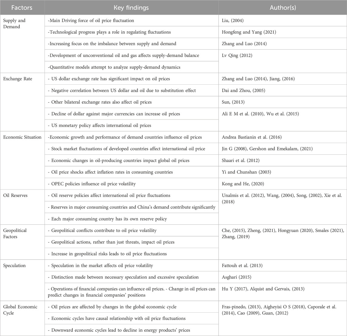
Table 1. Factors influencing oil price fluctuation.
As early as 1982, Engle pioneered the use of autoregressive conditional heteroscedasticity (ARCH) models to capture the persistence and aggregation of volatility. Since then, the generalized autoregressive conditional heteroscedasticity (GARCH) model developed by Bollerslev (1986) has become the basis of volatility analysis and has been combined with stochastic volatility model. Over time, GARCH-like models have been widely applied and expanded, such as Nelson’s (1991) exponential GARCH variant, Engle et al. (1993) asymmetric GARCH, Özdemir, 2022 and Liu et al. (2021) GARCH-MIDAS etc.
However, as Schwert (1989) points out, stock market volatility is related to macroeconomic activity. Empirical evidence suggests that a model in the form of long-term volatility factor can better describe volatility. Thus, the scientific community has proposed several models to achieve this goal. Engle et al. (1993) developed an additive equal-drift volatility model in which the long-run mean component and the short-run transition component were modeled by different GARCH (1,1) processes. Others also proposed various two-factor models: Ding and Granger (1996) proposed a long memory model, Alizadeh and Diebold (2002) used the basic stochastic volatility model of price range to target volatility, and Chernov et al. (2003) considered multiple stochastic volatility factors.
Despite numerous innovations, the major innovations in GARCH-type processes came in 2008 and 2013. In 2008, Engle and Rangel (2008) proposed the multiplicative bivariate GARCH, which uses gradually changing deterministic variables and short-term GARCH. Adrian and Rosenberg (2008) considered the addition model of short- and long-term volatility. In 2013, Engle, Ghysels and Sohn (2013) developed the GARCH-MIDAS (Mixed Data sampling) model, which enables low-frequency macroeconomic data to be directly included in the long-term volatility composition. Specifically, this model utilizes the standard GARCH (1,1) process when modeling short-term volatility, and the MIDAS term developed by Ghysels et al. (2006) is used to establish the long-term process. Engle found that the macroeconomic factor they selected contributed about 30% to volatility in the short run, while it contributed about half of the predicted volatility in the entire sample. Moreover, the predictive power of macroeconomic factors is even more advantageous when taking a longer-term view. By comparing the mean square error of the model containing macroeconomic variables with the sample GARCH model, it is found that the GARCH-Midas model has better prediction effect.
Since its inception in 2013, the GARCH-MIDAS model has found application across diverse contexts. Asgharian et al. (2013) extended the analysis of macroeconomic impacts by transforming principal components of macroeconomic factors into dimensions. Conrad and Loch (2015), however, applied the GARCH-MIDAS model to macroeconomic variables in the United States and found that these variables have an important impact on volatility. They classified them into priority (e.g., housing, starts, etc.) and secondary variables related to volatility according to their weighting scheme. Furthermore, the inverse periodicity reflecting volatility is optimized.
In the Chinese market, Girardin and Joyeux (2013) studied the relationship between inflation and production elements, while Wei et al. (2017a) explored the effect of “hot money.” In the study of emerging things, Conrad et al. (2018) analyzed the influence of long-term components on the volatility of cryptocurrency. Jebran et al. (2017) suggests that using the Grach model can effectively investigate the relationship between oil prices and stock market volatility. In addition, many applied studies of GARCH-MIDAS focus on commodity analysis, such as the volatility of agricultural prices studied by Donmez and Magrini (2013), the volatility of oil prices and the characteristics of supply and demand studied by Pan et al. (2017). The impact of US monetary policy on oil volatility studied by Amendola et al. (2017), and the impact of economic policy uncertainty on oil volatility studied by Wei et al. (2017b).
Most of the literature shows that macroeconomic variables have a significant effect on the volatility series studied. More importantly, these research all found that the GARCH-MIDASs model incorporating long-term volatility variables is more accurate than the basic GARCH model. At present, the parameter simplification of macroeconomic variables in GARCH-MIDAS model is still controversial. While current literature suggests using the variance of macroeconomic variables for parameter simplification, analysis and comparison indicate minimal improvement in forecasting ability. However, the model confidence set method of Wei et al. (2017a) may be an ideal solution to simplify the parameters.
Despite the inclusion of long-run macroeconomic components, Engle et al. (2013) still find that “the full-sample model is not immune to disruption” when industrial production indices and inflation are used as factors. Consequently, they had to break down the parent sample into subsamples to improve the fit. Many researchers have found that there are structural mutations in the process of asset price fluctuations. This problem was discovered by Andreou and Ghysels (2002), who found structural mutations in parameters related to the Russian and Asian crises. The fact that the GARCH-MIDAS model fails to consider structural mutations is a major limitation, as demonstrated by Bai and Perron (1998), for which most mutations can only be identified after the fact with multiple test methods. Therefore, To accurately predict volatility, it is better to take structural changes into account in the model itself.
One approach to normalize and refine prediction accuracy is by integrating potential mutations into the model’s state-transition mechanism. Weight, a unique form of structural mutation, depends on data probability derived from each potential volatility process activated in each period, leading to discrete volatility transitions. Therefore, the weight model can be used to simulate the volatility, especially the double weight model which originates from the inverse periodicity of the volatility. Volatility tends to increase during recessions and stay low over the course of upcycles. Therefore, two GARCH processes with different unconditional variances can embody the volatility process. As Hamilton and Lin (1996) found, the use weight method can lead to higher volatility during recessions.
Hamilton (1989) introduced the model transformation model based on Markov process determination into economics, resulting in several key achievements in the field of volatility modeling. Researchers like Diebold (1986), Lamoreux and Lastrapes (1990), and Kim and Kon (1999) found that the persistence parameter of GARCH process was reduced by introducing different modes into GARCH process. So, ignoring these changes can lead to misprediction of the model. After research, Mikosch and Starica (2004) and Hillebrand (2005) both found the same problem, that is, the process of continuously reaching stability in the GARCH (1,1) model is non-stationary due to the “unconditional variance change.” This suggests that several different GARCH (1,1) procedures can be applied to capture changes in unconditional variance over the course of short-term fluctuations.
Hamilton and Susmel (1994) verified this weight change model and found that it improved the accuracy of fitting and prediction and distinguished the difference between high-volatility and low-volatility variablesbut failed to deal with the attenuation problem of high-volatility variables. Klaassen (2002) applied the macro variable conversion model developed by Gray (1996) to the study of US dollar exchange rate and solved the problem of excessive volatility of univariate forecast. On the other hand, Haas et al. (2004) found that in some specific cases, model estimation results are not significant, so not all volatility variables can be predicted by the model.
In general, this section mainly discusses the development and evolution of the GARCH model, as well as the application and challenges of the GARCH-MIDAS model (Table 2). The GARCH-MIDAS model can directly incorporate low-frequency macroeconomic data into the long-term volatility component, thereby enhancing the model’s predictive ability. Although the GARCH-MIDAS model has been widely applied in various fields, it still faces some challenges, such as limitations in considering structural changes and parameter simplification. Therefore, further research on how to overcome these challenges and improve the accuracy and applicability of the model is of great significance.
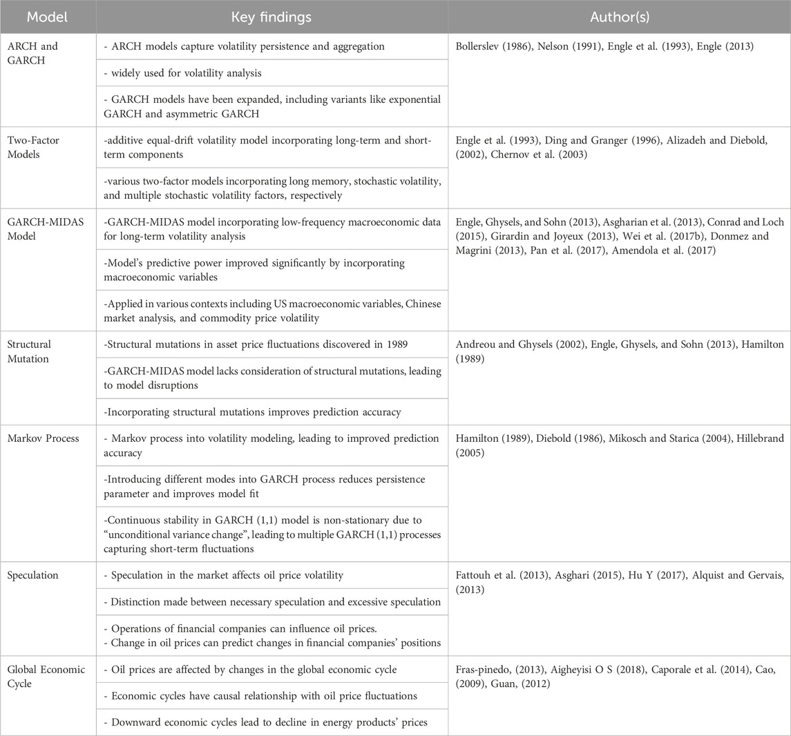
Table 2. Key models and findings in volatility theory.
The factors influencing oil price fluctuations encompass geopolitical risk, economic growth, exchange rate fluctuations, global inflation, stock market performance, monetary policy, speculation, business cycles, the global economy, and the development of major oil and gas-consuming countries. However, the proportion and priority of the influence of various factors on WTI oil have not been comprehensively evaluated. Notably, different factors exhibit varied correlations with the degree of impact on WTI oil across different fluctuation ranges, which is also contingent upon the price range of WTI oil. Therefore, the comprehensive consideration of the relationship between various factors and WTI oil volatility becomes a big difficulty.
Through the research on the theoretical status of volatility, it is found that GARCH-MIDAS is the mainstream model that synthesizes high-frequency data and low-frequency data, and a variety of models can cope with a variety of market situations. However, GARCH-MIDAS has not been used in the relevant literature to study the volatility of oil, which has not involved the huge volatility of WTI oil market since 2020. Therefore, there is still a large room for improvement of the relevant model theory. This paper aims to investigate the volatility of WTI crude oil prices during the observation period, yet all the models used previously fail to cover the period under study. Based on this, the paper poses the research question: The interference and influence of low-frequency variables on WTI crude oil volatility. Building upon this question, this study employs the GARCH-MIDAS model proposed by Engle et al. (2013), which is a single low-frequency variable model capable of discerning patterns to achieve the research objectives. The GARCH-MIDAS model is utilized to analyze the volatility of WTI oil at the present stage. Moreover, various low-frequency factors are incorporated to explore their impact on WTI oil volatility. The process is to select several representative low frequency factors, decompose the volatility into long-term and short-term components and realize frequency mixing, and establish a model for the single low frequency factor accordingly. Finally, according to the empirical results, the impact of each low frequency factor on the volatility of WTI oil market is studied, and relevant conclusions are drawn.
For the choice of volatility model, GARCH-MIDAS model proposed by Engle et al. (2013) is used in this paper. The model extracts two components of volatility: a short-term component reflecting mean reversion to high-frequency variables, and a long-term component incorporating low frequency explanatory variables using a beta weighting scheme. The average daily logarithmic rate of return of WTI is set as ri,t, where i is the high-frequency variable period, and the unit of i is day because the daily closing price of WTI is used for high-frequency data in this paper. It denotes the low frequency variable period, which is measured in months, quarters or years depending on the observed variable. Then there is:
Where,
High-frequency short-term variables are subject to GARCH (1,1) process, namely:
Among them, α and β are residual lag term coefficients and volatility lag term coefficients to be estimated, respectively, satisfying α > 0, β > 0, α+β < 1 and E (
Low-frequency long-term variable
where K > 0, its meaning is the hysteresis period of low-frequency long-term variable X weighted by the MIDAS weighting function. Variable X belongs to the macroeconomic variables introduced in the index data part, and Xt-k represents the rate of change of low-frequency long-term variables in the t-k month. Guerin and Marcellino (2013) discovered a serious non-convergence problem with the increase in the number of parameters in the MIDAS model. Hence, this paper refrains from considering the addition of more than one low-frequency long-term variable. m is the intercept term, θ is the slope of the influence of the lag term of the weighted low frequency variable on the long-term fluctuation of WTI oil, and K is the maximum lag order for smoothing the volatility in MIDAS filtering, which varies according to the low frequency variable used.
There are only two weight variables in this formula, namely
Therefore, a constraint of
So the decline rate of the function is determined by the size of
In conclusion, GARCH-MIDAS used maximum likelihood estimation to obtain parameter values to be estimated, and the parameter space was denoted as Θ = {µ, α, β, m, θ, ω}. Then there is maximum likelihood value LLH:
Given that oil volatility is influenced by various factors, the actual data presents obvious asymmetry. Therefore, the asymmetry effect is introduced into the GARCH-Midas model, and the high-frequency short-term variable process is modified from the standard GARCH(1,1) to the GFR-GArch model, namely:
Among them, α and β are residual lag term coefficients and volatility lag term coefficients to be estimated, which satisfy α > 0, β > 0, α+β+γ/2<1 and E (
Similarly, GJR-GARCH-MIDAS used maximum likelihood estimation to obtain the parameter values to be estimated, denoted as Θ = {µ, α, β, γ, m, θ, ω}. The formula of maximum likelihood value is the same as Eq. 6.
Before the sample is tested, the sample data is divided into observation sample and prediction sample. Model parameter estimation and comparison of model fitting effectiveness are performed based on the observation sample, while the prediction sample is reserved for evaluating prediction accuracy beyond the sample period.
A total of 3,340 sample data pieces are provided in this paper, spanning from 1 December 2009, to 4 October 2022. The first 2,840 pieces of data are used as observation samples, and the last 500 pieces of data are used as prediction samples. Data statistics and analysis are carried out based on this method.
The maximum likelihood estimation method is employed to determine parameter values from the observed samples. Subsequently, the GARCH-MIDAS model utilizes these parameter values to predict the first set of values. The prediction errors are then compared with the predicted sample. Then, the method of rolling time window is used to delete the first sample data in the observation sample, and the predicted data is added to the end of the observation sample. GARCH-MIDAS model was used again to predict the second predicted value. Repeat the above steps until the predicted value is dated 4 October 2022, and you have 500 out of sample predicted values. By comparing the predicted value of 500 volatilities with the actual value of volatilities in the forecast sample, the out-of-sample predictive ability of each model can be compared. The smaller the error is, the better the prediction ability of the prediction model is.
To effectively address this issue, loss functions are employed. As there are many types of loss functions, the academic circle has not clearly indicated which is the most effective loss function at present, so this paper selects four commonly used loss functions as the criteria to judge the prediction accuracy of the model in the empirical analysis. The four loss functions are mean absolute error (MAE), mean absolute percentage error (MAPE), square of mean error (MSE) and Gaussian quasi-maximum likelihood loss function error (QLIKE). Their function expressions are as follows:
In the formula, RV represents the realized volatility of WTI oil market, and the calculation formula is:
where,
In addition, Bayesian information criterion values BIC and maximum likelihood value LLH were used to evaluate the adaptability of the model in describing WIT oil market volatility. The smaller the BIC and LLH values were, the better the model was described.
In this study, the logarithmic yield of the daily closing price of WTI oil is selected as the high frequency variable. The selected timeframe spans from 1 December 2009, to 4 October 2022, comprising a total of 3,340 data points. The initial 2,840 data are taken as in-sample data, and the last 500 data are taken as out-of-sample data to verify the model effect. Figures 1, 2, respectively show the closing price trend chart of WTI oil and the logarithmic yield chart of the closing price of WTI oil. As can be seen from the figure, the oil price was relatively stable from 2010 to 2013, and then entered the downward trend. The average daily volatility of oil was basically within 10% before 2020, followed by several large fluctuations in a period. Due to the relatively low oil prices during these fluctuation cycles, the magnitude of the oil price’s substantial fluctuations is not readily apparent from the oil price chart.
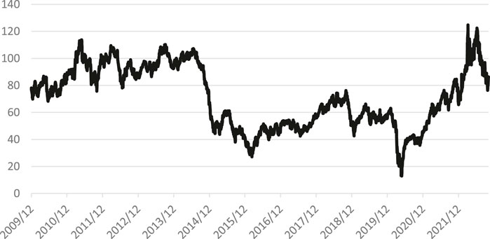
Figure 1. WTI oil price trend chart. Data source: The data in the figure above is from Choice financial terminal.
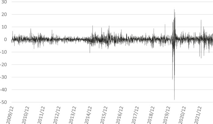
Figure 2. WTI oil price logarithmic yield chart.
In order to better analyze the sample data, descriptive statistical analysis is carried out on the data of each economic variable. The high-frequency data rWTI is the hundredfold product of the logarithmic yield of WTI international oil. Drawing from the literature review, the pivotal factors identified for this study encompass the consumer price index (CPI) (Engel and Rangel, 2008), industrial production index (IPI) (Amendola et al., 2017), rig drilling numbers in oil storage (ADU) (Unalmis et al., 2012), geopolitical risk (GPR) (Samles, 2021), and economic policy uncertainty (GEPU) (Wei et al., 2017a).
This paper mainly conducts descriptive statistical analysis of sample data from the indexes of mean value, standard error, skewness, kurtosis, maximum value, minimum value, etc. Table 3 shows the results of descriptive statistical analysis of sample data. According to the results in Table 3, it can be concluded that WTI international oil is left-skewed, but the kurtosis is greater than 3, indicating that the volatility of WTI international oil yield has the characteristics of “sharp peak and thick tail.” In terms of macro variables, the mean value of CPI is 2.36796 and the standard deviation is 1.951764, indicating that the CPI in the United States has a small change range and is in a basically stable state. At the same time, the distribution of CPI data is asymmetrical, and the right tail is too long, which is skewed to the right. The mean value of industrial production index IPI is 98.80771, the standard deviation is 4.625571, the skewness is −0.62313, and the kurtosis is less than 3, indicating that the distribution of the data is close to the normal distribution and the data distribution is relatively stable.
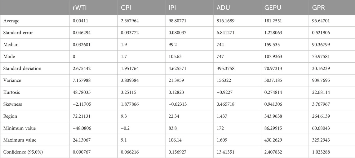
Table 3. Parameter description statistics table.
The standard deviation of ADU, representing the number of drilling rigs globally, is 395.3758, signifying a wide fluctuation range and uneven data distribution. Similarly, the standard deviation of the GEPU index is 70.97313, reflecting a favorable dispersion effect. Conversely, the skewness of the GPR index is 3.767967, pointing to a significant extension of the right tail of the data distribution above the mean, characteristic of geopolitical risks. From these data, the six indicators have a large range of changes and are evenly distributed, and there is no obvious bias phenomenon except GPR, indicating that the results are highly reliable.
To verify the adaptability of the model to oil price fluctuations in the selection period, this paper selected two GARCH-MIDAS models, which are widely used, for comparative analysis. Using CPI as test sample, the applicability of traditional GARCH-MIDAS model and asymmetric GJRGARCH-MIDAS model in the prediction of WTI oil volatility was tested. Through the calculation of the mixing model, the results are shown in Table 4. It can be seen from the table that the parameter estimates of the two models are significant, and the Log-lik values are −6,630 and −6,586, respectively. According to the Bayesian information criterion (BIC), it can be shown that although the results of the two models are close under long-term simulation conditions, However, the asymmetric GJRGARCH-MIDAS model is slightly better than the traditional GARCH-MIDAS model in sample fitting.
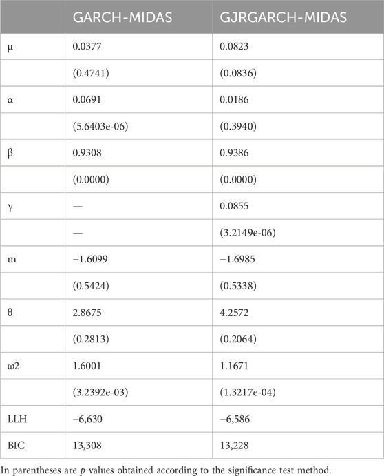
Table 4. Model comparison results.
The two models are used to predict the out-of-sample data, and the results are shown in Figure 3. It can be observed from the figure that the mixing volatility results of the two models in the samples are similar. However, in the comparison of long-term volatility, the asymmetric GJRGARCH-MIDAS model has greater volatility than the traditional GARCH-MIDAS model, while the traditional GARCH-MIDAS model shows greater volatility in the short-term volatility. GARCH-MIDAS series models are characterized by introducing long-term variables into the model to analyze the impact of long-term factors on target volatility. Therefore, the asymmetric GJRGARCH-MIDAS model, which is more sensitive to long-term variable data, better suits the needs of this empirical study. Additionally, it can be observed that in the prediction of out-of-sample data, the two models have good fitting effect, among which the asymmetric GJRGARCH-MIDAS model is closer to the actual realized rate of return and more accurate for the later prediction results. Therefore, this paper selects the asymmetric GJRGARCH-MIDAS model as the basic model for the subsequent simulation.
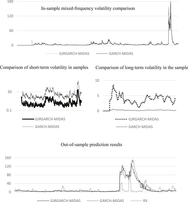
Figure 3. Comparison of the two models.
The mixing model is performed for each factor and the estimated results reflect the influence of each influencing factor on the long-term component of high frequency volatility on the level effect, which is the optimal estimated weight corresponding to the single factor mixing level value model. Therefore, it is determined that the maximum lag order K of the optimal MIDAS filtering of each model is 12 cycles. Based on this, GJRGARCH-MIDAS analysis is conducted on all low-frequency variables in this paper, and Table 5 is obtained as follows:
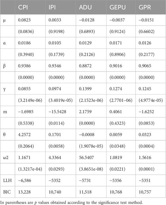
Table 5. Estimation results of GJRGARCH-MIDAS model for the full sample of each parameter.
The above table shows the simulation results of GJRGARCH-MIDAS model. All parameters satisfy α > 0, β > 0, and α+β+ γ/2 < 1, indicating that the GJRGARCH-MIDAS model is stable, and the volatility of WTI oil market tends to converge.
The first column of Table 5 is analyzed to study the impact of CPI on WTI oil market volatility. According to the estimated results: The influence coefficient θ of CPI on the long-term component of WTI oil market volatility is 4.2572, indicating that when CPI rises, it has a strong stimulating effect on the long-term component of WTI oil market volatility, and the relationship between the two is positively correlated. The absolute value indicates that the level direction of CPI has a great influence on the volatility of WTI oil market. In the estimation weight function (Eq. 5), the ω1 value is set to 1 to increase constraints, and the other parameter estimation value of the weight polynomial, ω2, is 1.1671. This indicates that the curve of the weight polynomial is relatively flat, suggesting that CPI has a long-term impact on the volatility of the WTI oil market and will maintain a positive correlation over a period. It also indicates that CPI has a weak effect on the short-term volatility of the WTI oil market.
The second column of Table 5 is analyzed to study the impact of IPI on the volatility of WTI oil market. According to the estimated results, the influence coefficient θ of IPI on the long-term component of WTI oil market volatility is 0.1701, indicating that IPI index has a weak stimulating effect on the long-term component of WTI oil market volatility when it rises.
The relationship between the two is positively correlated, and the absolute value indicates that the horizontal direction of IPI has a weak influence on the volatility of WTI oil market. The estimated value of the weight polynomial parameter, ω2, is 4.3364, indicating that the curve regression of the weight polynomial is slightly rapid, indicating that t IPI has a more direct influence on the volatility of WTI oil market.
The third column data in Table 5 is analyzed to study the influence of the current global rig spud number ADU on the volatility of WTI oil market. According to the estimated results, the influence coefficient θ of ADU on the long-term component of WTI oil market volatility is −0.0008, revealing a negative correlation, indicating that the increase in the number of drilling RIGS has a relative inhibitory effect on WTI oil market volatility. The absolute value indicates that the change of drilling rig number has a weak influence on the volatility of WTI oil market. The estimated value of the weight polynomial parameter, ω2, is 56.5407, indicating that the curve of the weight polynomial is extremely steep, indicating that the global drilling rig count has a more direct impact on the volatility of the WTI oil market. Moreover, it highlights the heightened sensitivity of short-term volatility in the WTI oil market to fluctuations in the global drilling rig count.
The fourth column of Table 5 is analyzed to study the influence of global economic policy uncertainty index GEPU on the volatility of WTI oil market. According to the estimated results, the influence coefficient θ of GEPU on the long-term component of WTI oil market volatility is 0.0059, indicating that the change of GEPU has a relatively stimulating effect on the volatility of WTI oil market, and the two present a positive correlation. The absolute value indicates that the change of GEPU has a weak influence on the volatility of WTI oil market. Moreover, the estimated value of the weight polynomial parameter, ω2, is 1.0819, indicating that the curve of the weight polynomial is relatively flat. This observation indicates that GEPU has a more profound influence on the volatility of the WTI oil market. Additionally, it implies that the short-term volatility of the WTI oil market is weakly influenced by GEPU.
The fifth column of Table 5 is analyzed to study the influence of geopolitical risk index GPR on the volatility of WTI oil market. According to the estimation results, the influence coefficient θ of GPR on the long-term component of WTI oil market volatility is 0.0323, and the two show a positive correlation. Its absolute value is much higher than that of GEPU, suggesting that changes in GPR will stimulate the volatility of WTI oil market more than changes in GEPU. The estimated value of the weight polynomial parameter is 1.5616, which indicates that the curve of the weight polynomial of GPR is slightly more erratic than that of GEPU, indicating that the influence of GPR on the short-term volatility of WTI oil market is more obvious than that of GEPU.
Based on the above analysis, the corresponding preliminary conclusion is drawn, namely, the relationship between the five low-frequency variables explored in this paper and the long-term volatility of WTI oil. Then, the relationship between each variable and the long-term volatility of WTI oil is analyzed in detail with the graph.
Figure 4 shows the interpretation results of CPI forecast using GJRGARCH-MIDAS model. The figure above left shows the in-sample fitting effect of GJRGARCH-MIDAS model based on CPI level value. Due to the extreme allocation of WTI oil volatility in the first half of 2020 due to the epidemic and Russia-Ukraine conflict, the vertical axis in the figure was changed to a logarithmic coordinate system. The graph illustrates that the CPI-based model generally captures the volatility trend of WTI oil, albeit some extreme points remain inadequately fitted. The upper-right is the result of out-of-sample prediction based on in-sample data. It indicates that the predicted fluctuation trend closely aligns with reality, albeit the corresponding attenuation period notably falls short of the realized return rate. The lower left figure compares the mixing volatility with the long-term volatility in the model, and the long-term component has a positive contribution to the overall volatility. Finally, the lower-right figure illustrates the changes in the weight function within the long-term part of the model, demonstrating a tendency towards smooth convergence.
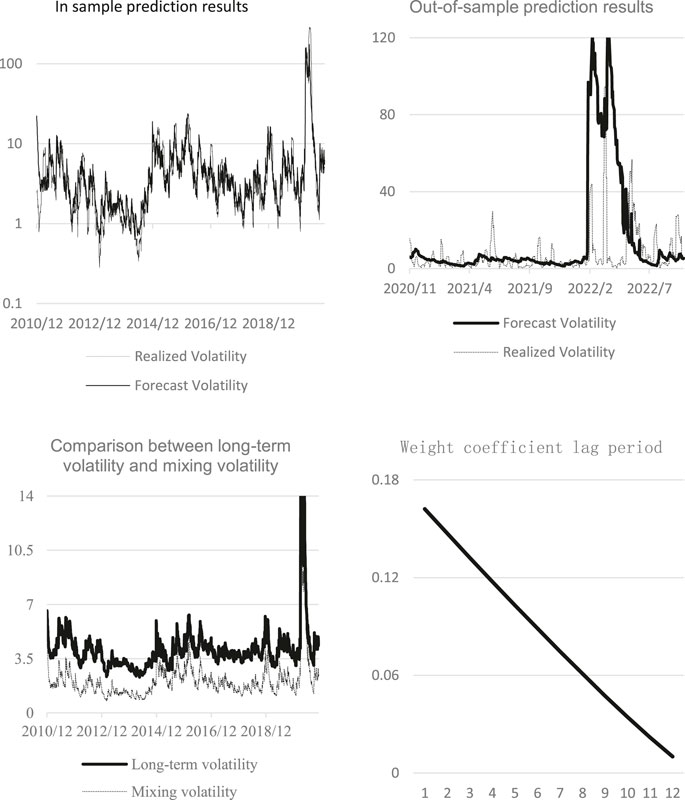
Figure 4. GJRGARCH-MIDAS model forecast of CPI.
Figure 5 shows the interpretation results of IPI prediction by GJRGARCH-MIDAS model. The figure above left shows the in-sample fitting effect of the GJRGARCH-MIDAS model based on IPI horizontal values. For reasons consistent with CPI, logarithmic coordinate system is used for the vertical axis in the figure. It is apparent from the graph that the IPI-based model has essentially captured the volatility trend of WTI oil, although some extreme points remain insufficiently fitted. Moving to the upper-right segment, it presents the outcomes of out-of-sample forecasting based on in-sample data. It can be seen that it is basically consistent with the result of CPI. The predicted fluctuation trend is basically close to the reality, but the attenuation period is too long. The lower-left figure compares the mixing volatility and long-term volatility in the model, revealing that the long-term component of IPI is more stable than that of CPI. The figure below on the right is the change chart of the weight function in the long-term part of the model. It can be seen that the weight of the model decreases sharply in the early stage and tends to be stable in the later stage, and the weight value is greater than the corresponding result of CPI.
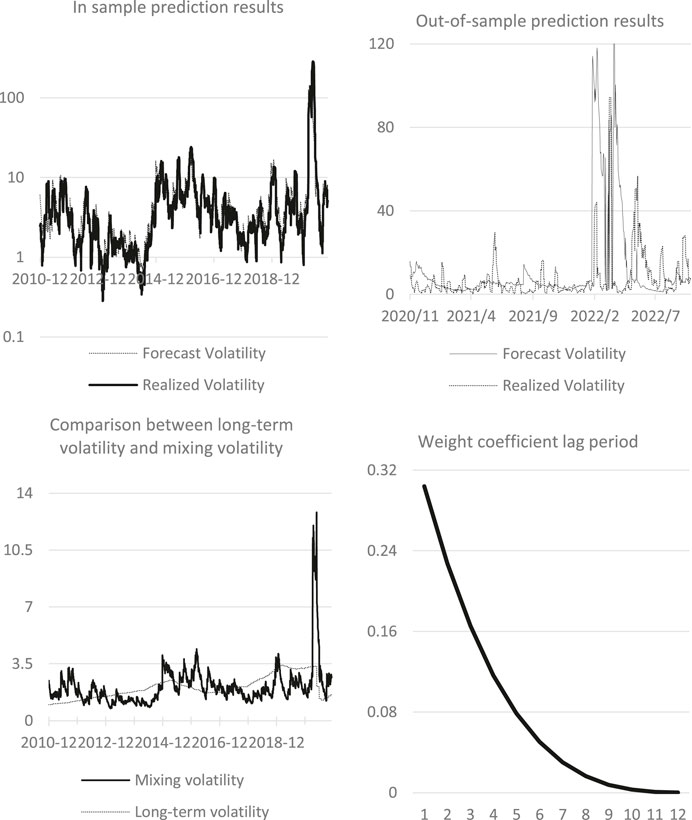
Figure 5. Prediction by GJRGARCH-MIDAS model of IPI.
Figure 6 shows the interpretation results of ADU prediction by GJRGARCH-MIDAS model. The above left figure shows the in-sample fitting effect of GJRGARCH-MIDAS model based on ADU level value. Since ADU is weekly frequency data, it can be observed that it changes more frequently, but the simulation of extreme volatility points needs to be improved. The figure on the right is the result of out-of-sample prediction based on in-sample data. It indicates that.
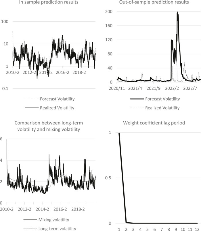
Figure 6. GJRGARCH-MIDAS model prediction of ADU.
ADU has predicted the trend of strong volatility, and its extreme value of volatility has far deviated from the realized volatility, indicating that it is difficult to predict the model under extreme conditions of WTI oil drastic fluctuations. Even short-term parameters are difficult to simulate accurately. The lower-left figure compares the mixing volatility with the long-term volatility in the model, highlighting that the long-term component of ADU is more stable than other parameters. The figure below on the right is the weight function change chart in the long-term part of the model. It demonstrates a sharp attenuation in the weight of the model, indicating that the impact of this parameter on the volatility of oil is relatively severe and short-lived.
Figure 7 shows the interpretation results of GEPU prediction using GJRGARCH-MIDAS model. The above left figure shows the in-sample fitting effect of GJRGARCH-MIDAS model based on GEPU level values. The above figure on the right is the result of out-of-sample prediction based on in-sample data. It is evident that GEPU predicted the trend of strong fluctuation, with its extreme value of fluctuation was the largest among all parameters, reflecting a strong warning effect. The lower left figure compares the mixing volatility with the long-term volatility in the model revealing that the long-term composition of GEPU is relatively smooth. The figure below on the right shows the weight function changes in the long-term part of the model. It shows that the weight of the model is relatively low, indicating that the long-term component has weak help to the model.
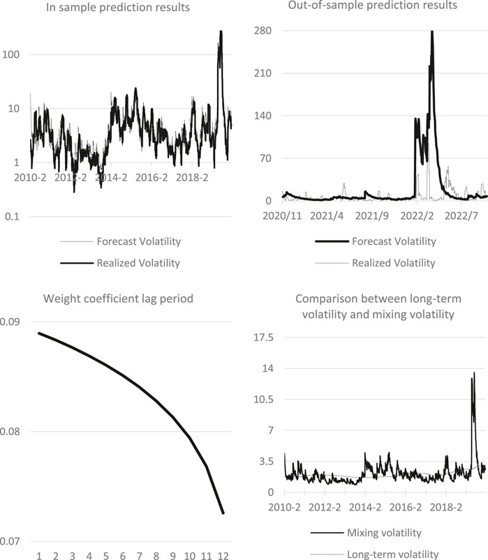
Figure 7. GJRGARCH-MIDAS model prediction of GEPU.
Figure 8 shows the interpretation results of GPR prediction by GJRGARCH-MIDAS model. The above left figure shows the in-sample fitting effect of GJRGARCH-MIDAS model based on GPR horizontal value. It can be observed that the fitting result of GPR is very close to GEPU. The above right is the result of out-of-sample prediction based on in-sample data. It can be noted that the prediction result of GPR is like that of other models, and the amplitude is similar to that of IPI. The lower left figure compares the mixing volatility with the long-term volatility in the model. It can be observed that the long-term component of GPR can affect the overall volatility in the region of low volatility. The figure below on the right shows the weight in the long-term part of the model. Although the attenuation speed is slow, the influence is long-term, but the weight proportion of GPR is the lowest among all variables.
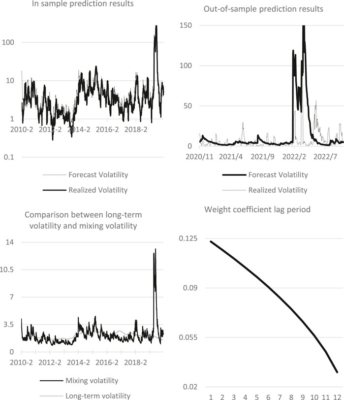
Figure 8. GJRGARCH-MIDAS model prediction of GPR.
Compare the errors between the mixing volatility calculated by the model using each low frequency variable and the realized volatility calculated by using the original data, to compare the advantages and disadvantages of the model. The four loss functions mentioned in Chapter 2 are used to test each parameter model. The loss function of each parameter is shown in Table 6.
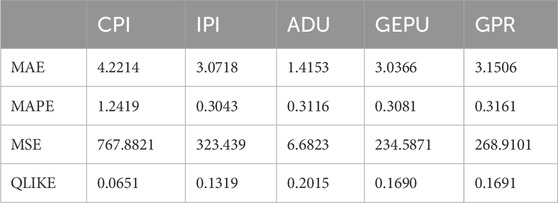
Table 6. Loss function of each parameter.
As shown in Table 6, MAE, MAPE, MSE and QLIKE are evaluated by four different evaluation indicators on the performance of five different models. For WTI international oil, the performance of all models is relatively good, among which, the performance of ADU model is excellent, achieving the minimum value in MAE and MSE loss functions, which is far lower than other indicators. When judging by MAPE method, the other four indicators are close except CPI which is poor. When QLIKE is used to judge, CPI performs much better than other indicators. After comprehensive comparison, the accuracy of the model is in the order of GEPU>ADU>IPI>GPR>CPI. In addition, according to the Bayesian information criterion values BIC and maximum likelihood value LLH in Table 5, all models have relatively good effects in describing the WIT oil market volatility. Except the CPI model, which slightly deviates from other models, the other models have similar BIC and LLH values. From the above out-of-sample forecast results, economic policy uncertainty has a significant impact on the future volatility of oil prices, followed by the number of global drilling RIGS, industrial production index, geopolitical risk index and consumer price index.
This study delves into the multifaceted determinants of international oil price fluctuations, identifying various factors and their interplay. The influencing factors encompass geopolitical risks, economic growth, currency dynamics, inflation, stock market performance, monetary policies, speculation, business cycles, global economic conditions, and the behaviors of major oil-consuming nations. These factors exhibit interconnectedness or correlation, forming a complex web of influences on oil price volatility.
To comprehensively understand the dynamics, the study focuses on five representative low-frequency variables and assesses their contributions to oil price fluctuations. Employing the GARCH-MIDAS model, correlations among these factors are analyzed, shedding light on their impacts on oil price volatility. During the study period, the WTI international oil price has a relatively stable cycle, but also has a huge fluctuation cycle. In this paper, the GARCH-MIDAS model of various low frequency variable factors was tested by Bayesian information criterion BIC and maximum likelihood number LLH. All the models demonstrated good estimation effect. The long-term component of the model can identify the fluctuation trend of oil price correctly. However, the fluctuation value in extreme condition is much different from the actual value. Additionally, four loss functions are introduced: MAE, MAPE, MSE and Gaussian quasi-maximum likelihood loss function error. Four loss functions were used to test the model and the accuracy was evaluated among the models. The empirical analysis mainly draws the following conclusions:
(1) The GARCH-MIDAS model proves to be particularly effective in accurately predicting the volatility of oil during periods of relatively smooth fluctuations in WTI international oil prices. Under the premise that the world economy and society are relatively stable in the future, GARCH-MIDAS model can effectively simulate the fluctuation trend of WTI international oil prices. However, during periods of significant fluctuation in WTI international oil prices, although the GARCH-MIDAS model is employed and the fluctuation period is incorporated into the sample, it can only predict the general trend of fluctuations. The selection of low-frequency variables cannot be effectively corrected because low-frequency variables are more macroeconomic parameters and cannot respond effectively and timely to short-term shocks brought by large-scale international events. Low-frequency variables typically lag behind international oil prices in their response to such events. In contrast, oil price fluctuations tend to exhibit greater sensitivity and immediacy in response to specific events.
(2) In comparison to the two macroeconomic indicators selected in this study, namely the Consumer Price Index (CPI) and the Industrial Production Index (IPI), both exhibit similar trends in their influence on WTI international oil prices, albeit with varying degrees of impact. Through various tests and evaluations, IPI has a greater weight on the volatility of WTI international oil prices. This is consistent with the actual situation. Firstly, Industrial production index (IPI) is an important indicator to measure a country’s industrial production, which reflects the development of a country’s economy. The level of economic development directly correlates with oil consumption capacity, consequently impacting oil price fluctuation. Secondly, the Consumer Price Index (CPI) represents consumers’ actual purchasing power, reflecting changes in market demand. However, CPI is a comprehensive reflection of all product prices and does not target oil related products, so there is an error in the impact of international oil price fluctuations. As a result, international oil prices are more sensitive to indicators that are more closely related to them, and related indicators are better able to guide future fluctuations of international oil.
(3) Both the economic policy uncertainty index (GEPU) and the geopolitical risk index (GPR) offer macro-level insights into global conditions. Although there is a large gap between the simulation results of the two indexes by GARCH-MIDAS model, its guiding significance to the volatility of international oil prices still exists. The two indexes show relatively accurate fitting and fluctuation in the cycle of relatively stable oil price fluctuation, among which GEPU index and CPI index are faced with the same problem, and the feedback of economic policy uncertainty is limited to related policies directly related to oil price. Although economic policy uncertainty affects oil prices indirectly through factors such as the economy, exchange rates, inflation, stock markets, and monetary policy, the effective feedback cycle is relatively prolonged and weak. On the other hand, the fluctuation of its index still has positive guiding significance when other indicators are relatively peaceful. The GPR index reflects geopolitical risk, but the index data is released over a long period of time. During periods of geopolitical tension, changes in the GPR can indeed feed back into fluctuations in international oil prices. But after major geopolitical events, international oil prices respond much faster than the GPR. International oil prices are more sensitive to events, causing the GPR to fluctuate more slowly than large fluctuations in international oil prices. Therefore, the impact of geopolitical events on international oil price fluctuations cannot be judged by this index alone.
(4) The GARCH-MIDAS model with global drilling rig count as the low-frequency variable is the GARCH-MIDAs model with excellent comprehensive performance in this paper. It demonstrates the lowest synthesis of loss functions and exhibits the strongest sensitivity to WTI international oil price volatility. Moreover, the conclusion that it is negatively correlated with international oil prices has been corroborated. Although the number of global drilling RIGS is apparently decided subjectively by each oil company, it is fundamentally a comprehensive judgment made by each oil company based on the current oil price range and the macroeconomic policies and global political situation in the future period, the expectation of future oil price and market demand, and its own recoverable oil reserves, drilling production cycle, investment and income. Furthermore, it underscores the strategic interactions among oil companies and even nations. The industry is more sensitive to the judgment of oil price fluctuation and trend. However, due to commercial competition and other factors, information sharing among companies is limited, and future judgments and policy changes are not publicly disclosed. More variables like the number of global drilling RIGS are needed as relevant references. To understand the industry related companies in the future period of behavior. The warning for the internal enterprises of our country is also reflected in this point, that the relevant Chinese enterprises need to realize the internal cycle as soon as possible, reduce the dependence on foreign oil service enterprises, and improve the implementation of the overall industry data secrecy work.
Future research could further explore the multifaceted determinants of international oil price fluctuations and delve deeper into the interactions among these factors. The influencing factors encompass geopolitical risks, economic growth, currency dynamics, inflation, stock market performance, monetary policies, speculation, business cycles, global economic conditions, and the behaviors of major oil-consuming nations. These factors exhibit interconnectedness or correlation, forming a complex web of influences on oil price volatility.
Furthermore, considering the inclusion of additional low-frequency variables in the GARCH-MIDAS model could enhance its predictive capability. Further exploration of the relationships between international oil price fluctuations and global economic conditions, geopolitical risks, and other factors would provide comprehensive insights for predicting and managing future oil price fluctuations.
The original contributions presented in the study are included in the article/supplementary material, further inquiries can be directed to the corresponding author.
YL: Writing–original draft, Writing–review and editing. JW: Writing–original draft, Writing–review and editing. YW: Writing–original draft, Writing–review and editing. JL: Writing–original draft. YZ: Writing–original draft, Writing–review and editing.
The authors declare financial support was received for the research, authorship, and/or publication of this article. This work was supported in part by the National Natural Science Foundation of China Grant 71971177, and Dalian Commodity Exchange “Bai Xiao Wan Cai” Project (DECYJ202301).
The authors are grateful to the editors and referees for their valuable comments and suggestions on this paper.
The authors declare that the research was conducted in the absence of any commercial or financial relationships that could be construed as a potential conflict of interest.
All claims expressed in this article are solely those of the authors and do not necessarily represent those of their affiliated organizations, or those of the publisher, the editors and the reviewers. Any product that may be evaluated in this article, or claim that may be made by its manufacturer, is not guaranteed or endorsed by the publisher.
Adrian, T., and Rosenberg, J. (2008). Stock returns and volatility: pricing the short-run and long-run components of market risk. J. Finance 63 (6), 2997–3030. doi:10.1111/j.1540-6261.2008.01419.x
Aigheyisi, O. S. (2018). Oil price volatility and business cycles in Nigeria. Stud. Bus. Econ. 13 (2), 31–40. doi:10.2478/sbe-2018-0018
Ali, E. M., and Mohammad, S. (2010). The impact of the u.s. monetary policy on the oil prices and the oil revenues of the opec members. Iran. J. Econ. Res. (14), 81–109.
Alizadeh, S., Diebold, B., and Diebold, F. X. (2002). Range-based estimation of stochastic volatility models. J. Finance 57 (3), 1047–1091. doi:10.1111/1540-6261.00454
Alquist, R., and Gervais, O. (2013). The role of financial speculation in driving the price of oil. Energy J. (34), 3. doi:10.5547/01956574.34.3.3
Amendola, A., Candila, V., and Scognamillo, A. (2017). On the influence of US monetary policy on crude oil price volatility. Empir. Econ. 52 (1), 155–178. doi:10.1007/s00181-016-1069-5
Andrea, B., Conti, F., and Manera, M. (2016). The impacts of oil price shocks on stock market volatility: evidence from the G7 countries. Energy Policy 98 (98), 160–169. doi:10.1016/j.enpol.2016.08.020
Andreou, E., and Ghysels, E. (2002). Detecting multiple breaks in financial market volatility dynamics. J. Appl. Econ. 17 (5), 579–600. doi:10.1002/jae.684
Asghari, M. (2015). Essays on the role of speculation in the volatility of oil prices and oil futures risk premia. Houston: University of Houston.
Asgharian, H., Hou, J., and Javed, F. (2013). The importance of the macroeconomic variables in forecasting stock return variance: a GARCH-MIDAS approach. J. Forecast. 32 (7), 600–612. doi:10.1002/for.2256
Bai, J., and Perron, P. (1998). Estimating and testing linear models with multiple structural changes. Econometrica 66 (1), 47–78. doi:10.2307/2998540
Bollerslev, T. (1986). Generalized autoregressive conditional heteroskedasticity. Eeri Res. Pap. 31 (3), 307–327. doi:10.1016/0304-4076(86)90063-1
Cao, D. (2009). The impact of cyclical fluctuation of world economy on oil price fluctuation. Hunan: Hunan University.
Caporale, G. M., Ali, F. M., and Spagnolo, N. (2015). Oil price uncertainty and sectoral stock returns in China: a time-varying approach. China Econ. Rev. 34 (34), 311–321. doi:10.1016/j.chieco.2014.09.008
Che, S. (2015). Analysis on the mechanism of geopolitical influence on international crude oil price. Price Mon. (11), 3.
Chernov, M., Gallant, A. R., Ghysels, E., and Tauchen, G. (2003). Alternative models for stock price dynamics. J. Econ. 116 (1-2), 225–257. doi:10.1016/s0304-4076(03)00108-8
Conrad, C., Custovic, A., and Ghysels, E. (2018). Long- and short-term cryptocurrency volatility components: a GARCH-MIDAS analysis. J. Risk Financial Manag. 11 (2), 23–35. doi:10.3390/jrfm11020023
Conrad, C., and Loch, K. (2015). Anticipating long-term stock market volatility. J. Appl. Econ. 30 (7), 1090–1114. doi:10.1002/jae.2404
Cutcu, I., Cil, D., Karis, C., and Kocak, S. (2024). Determining the green technology innovation accelator and natural resources towards decarbonization for the EU countries: evidence from MMQR. Environ. Sci. Pollut. Res. 31, 19002–19021. doi:10.1007/s11356-024-32302-4
Dai, J., and Zhou, X. (2005). Dollar exchange rate, inflation and oil price. Int. Pet. Econ. 13 (2), 3.
Diebold, F. (1986). Modeling the persistence of conditional variances: a comment. Econ. Rev. 5 (1), 51–56. doi:10.1080/07474938608800096
Ding, Z., and Granger, C. (1996). Modeling volatility persistence of speculative returns: a new approach. J. Econ. 73 (1), 185–215. doi:10.1016/0304-4076(95)01737-2
Donmez, A., and Magrini, E. (2013). Agricultural commodity price volatility and its macroeconomic determinants: a GARCH-MIDAS approach. Luxembourg: Publications Office of the European Union.
Engle, R., Ghysels, E., and Sohn, B. (2013). Stock market volatility and macroeconomic fundamentals. Rev. Econ. Statistics 95 (3), 776–797. doi:10.1162/rest_a_00300
Engle, R. F., and Rangel, J. G. (2008). The spline-GARCH model for low-frequency volatility and its global macroeconomic causes. Rev. Financial Stud. 21 (3), 1187–1222. doi:10.1093/rfs/hhn004
Engle, ROBERT F., and Ng, V. K. (1993). Measuring and testing the impact of news on volatility. J. Finance 48 (5), 1749–1778. doi:10.2307/2329066
Fattouh, B. K., Kilian, L., and Mahadeva, L. (2013). The role of speculation in oil markets: what have we learned so far? Energy J. 34 (34), 7–33. doi:10.5547/01956574.34.3.2
Frias-Pinedo, I. (2013). Oil price shocks and the business cycle in Spain: is the 2008 financial crisis different? Appl. Econ. Int. Dev. 13 (2), 15–26.
Gershon, O., and Emekalam, P. (2021). Determinants of renewable energy consumption in Nigeria: a toda yamamoto approach. IOP Conf. Ser. Earth Environ. Sci. (1), 665. doi:10.1088/1755-1315/665/1/012005
Ghysels, E., Sinko, A., and Valkanov, R. (2006). MIDAS regressions: further results and new directions. Econ. Rev. 26 (1), 53–90. doi:10.1080/07474930600972467
Girardin, E., and Joyeux, R. (2013). Macro fundamentals as a source of stock market volatility in China: a GARCH-MIDAS approach. Econ. Model. 34, 59–68. doi:10.1016/j.econmod.2012.12.001
Gray, S. (1996). Modeling the conditional distribution of interest rates as a regime-switching process. Jounral Financial Econ. 42 (42), 27–62. doi:10.1016/0304-405x(96)00875-6
Guerin, P., and Marcellino, M. (2013). Markov-Switching MIDAS models. J. Bus. &Economic Statistics 31 (1), 45–56. doi:10.1080/07350015.2012.727721
Haas, M., Mittnik, S., and Paolella, M. (2004). A new approach to markov-switching GARCH models. J. Financial Econ. 2 (4), 493–530. doi:10.1093/jjfinec/nbh020
Hamilton, J. (1989). A new approach to the economic analysis of nonstationary time series and the business cycle. Econometrica 57 (2), 357–384. doi:10.2307/1912559
Hamilton, J., and Lin, G. (1996). Stock market volatility and the business cycle. J. Appl. Econ. 11 (5), 573–593. doi:10.1002/(sici)1099-1255(199609)11:5<573::aid-jae413>3.0.co;2-t
Hamilton, J., and Susmel, R. (1994). Autoregressive conditional heteroskedasticity and changes in regime. J. Econ. 64 (1), 307–333. doi:10.1016/0304-4076(94)90067-1
Hillebrand, E. (2005). Neglecting parameter changes in GARCH models. J. Econ. 129 (1), 121–138. doi:10.1016/j.jeconom.2004.09.005
Hongfeng, Xu, and Yang, Li (2021). Comprehensive analysis of international oil price: influencing factors, equilibrium points and energy cooperation between China and Russia. Russ. Central Asian East. Eur. Stud. (2), 52–74.
Hongyuan, Yu (2020). International oil price shocks and countermeasures from the perspective of geopolitics. Int. Outlook 12 (6), 24.
Hu, Y. (2017) The role of financial speculation in the world oil market: TVP-VAR and BVAR-SV approaches. Delaware: University of Delaware.
Jebran, K., Chen, S., Saeed, G., and Zeb, A. (2017). Dynamics of oil price shocks and stock market behavior in Pakistan: evidence from the 2007 financial crisis period. Financ. Innov. 3, 2–12. doi:10.1186/s40854-017-0052-2
Jiang, J. Q. (2016) Study on long-term cross correlation between international oil price and dollar exchange rate. Nanjing: Nanjing University of Finance and Economics.
Jin, G. (2008). The impact of oil price shock and exchange rate volatility on economic growth: a comparative analysis for Russia Japan and China. Res. J. Int. Stud. (8), 98–111.
Kim, D., and Kon, S. (1999). Structural change and time dependence in models of stock returns. J. Empir. Finance 6 (3), 283–308. doi:10.1016/s0927-5398(99)00005-5
Klaassen, F. (2002). Improving GARCH volatility forecasts with regime-switching GARCH. Empir. Econ. 27, 363–394. doi:10.1007/s001810100100
Kong, Y., and He, Xi (2020). Chen Chen OPEC+output policy choice and the medium and long-term trend of oil price Sino-foreign. Energy 25 (8), 7.
Lamoreux, C., and Lastrapes, W. (1990). Persistence in variance, structural change, and the GARCH model. J. Bus. Econ. Statistics 8 (2), 225–234. doi:10.2307/1391985
Lee, G., and Engle, R. F. (1993). A permanent and transitory component model of stock return volatility. Cointegration Causality Forecast. A Festschrift Honor Clive WJ Granger (1), 475–497.
Liu, J., Zhang, Z., Yan, L., and Wen, F. (2021). Forecasting the volatility of EUA futures with economic policy uncertainty using the GARCH-MIDAS model. Financ. Innov. 7, 76–19. doi:10.1186/s40854-021-00292-8
Liu, M. (2004). The change trend of the structure and pattern of international oil supply and demand. Asia-pacific Secur. Oceanol. Res. (3), 26–31.
Lv, Q. (2012). Formation mechanism of international oil price and Chinese oil security strategy. Sci. Technol. Square (8), 4.
Mikosch, T., and Starica, C. (2004). Nonstationarities in financial time series, the long-range dependence, and the IGARCH effects. Rev. Econ. Statistics 86 (1), 378–390. doi:10.1162/003465304323023886
Nelson, D. B. (1991). Conditional heteroskedasticity in asset returns: a new approach. Model. Stock Mark. Volatility 59 (2), 347–360. doi:10.2307/2938260
Özdemir, O. (2022). Cue the volatility spillover in the cryptocurrency markets during the COVID-19 pandemic: evidence from DCC-GARCH and wavelet analysis. Financ. Innov. 8 (1), 12. doi:10.1186/s40854-021-00319-0
Özkök, Y., and Çütcü, İ. (2022). Does fiscal federalism matter for economic growth? Evidence from the United States. Appl. Econ. 54 (24), 2810–2824. doi:10.1080/00036846.2021.1998337
Pan, Z., Wang, Y., Wu, C., and Yin, L. (2017). Oil price volatility and macroeconomic fundamentals: a regime switching GARCH-MIDAS model. J. Empir. Finance 43 (43), 130–142. doi:10.1016/j.jempfin.2017.06.005
Schwert, G. W. (1989). Margin requirements and stock volatility. J. Financial Serv. Res. 3 (2-3), 153–164. doi:10.1007/bf00122799
Shaari, M. S., Hussain, N. E., and Abdullah, H. (2012). The effects of oil price shocks and exchange rate volatility on inflation: evidence from Malaysia. Int. Bus. Res. 5 (9), 5. doi:10.5539/ibr.v5n9p106
Smales, L. A. (2021). Geopolitical risk and volatility spillovers in oil and stock markets. Q. Rev. Econ. Finance (1), 80.
Sun, J. B. (2013). Comprehensive Correlation analysis of the influence of dollar exchange rate and oil supply and demand factors on international oil price fluctuations -- Based on empirical analysis of WTI price fluctuations. Management (26), 1.
Unalmis, D., Unalmis, I., and Unsal, F. D. (2012). On the sources and consequences of oil price shocks: the role of storage. IMF Work. Pap. (12), 270.
Wei, Y., Liu, J., Lai, X., and Hu, Y. (2017b). Which determinant is the most informative in forecasting oil market volatility: fundamental, speculation, or uncertainty. Energy Econ. 68, 141–150. doi:10.1016/j.eneco.2017.09.016
Wei, Y., Yu, Q., Liu, J., and Cao, Y. (2017a). Hot money and China’s stock market volatility: further evidence using the GARCH-MIDAS model. Phys. A Stat. Mech. it’s Appl. 492 (492), 923–930. doi:10.1016/j.physa.2017.11.022
Wu, P.-C. P., Liu, S. Y., and Pan, S. C. (2015). The impact of monetary policy on oil price persistence: an application of the smooth regime-switching model. J. Int. Trade and Econ. Dev. 24 (1/2), 24–42. doi:10.1080/09638199.2013.848462
Xie, N., Xu, G., and Lin, B. (2018). Study on the impact of China's oil demand and global oil inventory on international oil prices. Contemp. Econ. Sci. 40 (4), 8.
Yi, Li, and Chunshan, F. (2003). Study on the influence of OPEC on international oil price. Tech. Econ. Manag. Res. (5), 2.
Yi, Z., Wang, Ke, and Lin, J. (2014). Correlation analysis of dollar exchange rate and international oil price trend. Int. Pet. Econ. (5), 9.
Zhang, K., and Luo, Y. (2014). World oil supply and demand situation in the new century from the perspective of surplus production capacity. Domest. Foreign Energy (4), 1–5.
Zhang, L. (2019). International crude oil prices fluctuate as geopolitical risks increase. Int. Finance Stud. (1), 1.
Zhang, Y., and Ma, B. (2010). Analysis on main controlling factors of international crude oil price. China Foreign Energy 15 (4), 6.
Keywords: oil, volatility, forecast, GARCH-MIDAS, influence variables
Citation: Le Y, Wen J, Wu Y, Liu J and Zhu Y (2024) Investigating factors influencing oil volatility: a GARCH-MIDAS model analysis. Front. Energy Res. 12:1392905. doi: 10.3389/fenrg.2024.1392905
Received: 28 February 2024; Accepted: 23 May 2024;
Published: 13 June 2024.
Edited by:
Yanchu Liu, Sun Yat-sen University, ChinaReviewed by:
Ibrahim Cutcu, Hasan Kalyoncu University, TürkiyeCopyright © 2024 Le, Wen, Wu, Liu and Zhu. This is an open-access article distributed under the terms of the Creative Commons Attribution License (CC BY). The use, distribution or reproduction in other forums is permitted, provided the original author(s) and the copyright owner(s) are credited and that the original publication in this journal is cited, in accordance with accepted academic practice. No use, distribution or reproduction is permitted which does not comply with these terms.
*Correspondence: Jing Wen, bWFnZ2lld2VuNTI1QG91dGxvb2suY29t
Disclaimer: All claims expressed in this article are solely those of the authors and do not necessarily represent those of their affiliated organizations, or those of the publisher, the editors and the reviewers. Any product that may be evaluated in this article or claim that may be made by its manufacturer is not guaranteed or endorsed by the publisher.
Research integrity at Frontiers
Learn more about the work of our research integrity team to safeguard the quality of each article we publish.