Data-driven active corrective control in power systems: an interpretable deep reinforcement learning approach

With the successful application of artificial intelligence technology in various fields, deep reinforcement learning (DRL) algorithms have applied in active corrective control in the power system to improve accuracy and efficiency. However, the “black-box” nature of deep reinforcement learning models reduces their reliability in practical applications, making it difficult for operators to comprehend the decision-making mechanism. process of these models, thus undermining their credibility. In this paper, a DRL model is constructed based on the Markov decision process (MDP) to effectively address active corrective control issues in a 36-bus system. Furthermore, a feature importance explainability method is proposed, validating that the proposed feature importance-based explainability method enhances the transparency and reliability of the DRL model for active corrective control.

1 Introduction

With the construction and development of the new-type power system, the transmission power of lines continues to increase. When power lines experience overload or voltage violations, the operational state of the power system may deviate or become unstable, often accompanied by an imbalance in power within sections, which threatens the safety and stability of the power system Fitzmaurice et al. (2010). Hence, it is crucial to implement precise measures to mitigate overloads and excessive currents in power lines, aiming to avert the initiation of cascading failures. The exploration of prompt and efficient active corrective methods holds considerable importance for ensuring the secure and steady functioning of the power system.

The application of AI technology in active corrective control for power systems can significantly enhance decision-making efficiency, high-dimensional data processing capabilities, and the level of intelligence in the power system. By establishing mechanisms for assisting safety operation decisions and autonomous knowledge learning, it can improve the response speed and efficiency of the power grid in handling exceptional and fault conditions, reducing the workload of manual scheduling. To address the issues with traditional active corrective methods such as computational efficiency, accuracy, and the handling of massive data, DRL, as an emerging AI technology, has been gaining widespread attention. Reference Xu et al. (2019) introduces a model-free DRL algorithm for solving formulated MDP and learning optimal adjustment strategies. Reference Xu et al. (2021) presents a simulation-driven graph attention-based reinforcement learning approach for robust active power corrective control. Reference Zhang et al. (2022) integrates grid topology information into neural networks using a graph attention-based DRL model for digital simulation of power system operation and control decisions. Reference Zheng et al. (2024) develops a two-stage model for ESS that respects the nonanticipativity of multistage dispatch, and implement it into a distributionally robust model predictive control scheme. Reference Zhang C. et al. (2023) proposes a central limit theorem-based method (CLTM) to overcome the conservatism of interval DC and AC power flow analysis under uncertainty of renewable power generation. Reference Hossain et al. (2021) proposes a graph convolution-based DRL model framework to address topological changes in power systems.

AI technology can enhance the efficiency and accuracy of active corrective control in power systems. However, corrective control demands a high level of safety and reliability. The decision-making process of AI models should be understandable and trustworthy so that human operators can intervene and make adjustments. In the research of interpretable methods for machine learning models in power systems, one widely used approach is feature importance Shrikumar et al. (2017), which analyzes the impact of features on the model to assess their importance and further understand the relationships between variables. Reference Wu et al. (2022) addresses the interpretable of a multi-factor wind speed prediction model in power systems. Reference Zhang et al. (2021) proposes the design of a key part of a visual heterogeneous information network for explaining model decisions in power systems. Reference Zhang K. et al. (2023) presented a graph deep reinforcement learning model applied to active power correction control and introduced a subgraph explanation method. Reference Liu et al. (2023) adopts the method of feature importance to explain and analyze the transient stability assessment process of power systems based on machine learning. Reference Ren et al. (2021) proposes using feature importance method to explain the decision results of transient stability preventive control model and identify the most effective control objects to reduce the number of control objects. Reference Yang et al. (2022) can predict the static voltage stability index online by correcting the control model, and calculate the approximate value of each characteristic sensitivity to the voltage stability index under any operating mode. Reference Mitrentsis and Lens (2022) uses the feature importance SHAP value method to explain the decision results of photovoltaic power prediction models. Reference Hamilton and Papadopoulos (2023) adopts the feature importance method to obtain the interpretation of machine learning models for location-specific transient stability assessment.

Explainable Artificial Intelligence (XAI) does not have a mathematical definition Molnar (2020), it can refer to the degree to which individuals can consistently predict model outcomes Kim et al. (2016). The higher the interpretability of machine learning, the easier it is for individuals to understand why certain decisions or predictions are made Molnar (2020). Specifically, XAI is a set of processes and methods that facilitate the understanding and trust of results and outputs computed by machine learning algorithms, presenting model decision outcomes in an easily understandable manner. It is essential for helping individuals comprehend the inner workings of complex models and how they make specific decisions. At the core of XAI is providing the rationale and execution logic for the decision-making process of artificial intelligence models, and visualizing these through a series of human-understandable means, thereby fostering trust in artificial intelligence models by humans.

In the process of active power corrective control of power system, operators can understand the contribution of model input features to output decision-making through XAI, and by combining experience and domain knowledge, operators can understand the causal relationship to improve the confidence and acceptance of operators on the DRL model of active power corrective control proposed in this paper.

This paper proposes the use of a Markov Decision Process (MDP) to establish a competitive Dueling Double Deep Q-network model (D3QN) to implement active corrective control in the power system. When facing scenarios such as “N-1” faults and fluctuations in supply and demand, it achieves the redistribution and rescheduling of active power among different generator units in the system, effectively addressing transmission line overloading issues. Additionally, a feature importance-based interpretable method (Deep-SHAP) is introduced to enhance the efficiency of feature importance calculations and provide explanations for the decisions made by DRL models in the context of active corrective control in the power system.

The remaining sections of this paper are structured as follows. In Section 2, we delve into the problem modeling aspect, encompassing corrective control objectives, constraints, and the formulation of the Markov Decision Process (MDP). Section 3 provides a comprehensive and interpretable overview of the proposed approaches, highlighting both the D3QN model and the Deep-SHAP method. Moving on to Section 4, we showcase the test cases along with their corresponding outcomes. Finally, Section 5 encapsulates our conclusions and outlines potential directions for future research.

2 Problem modeling

2.1 Corrective control objective function and constraints

While satisfying the operational constraints of the power grid, active corrective measures include adjusting the active output of generators, shedding a portion of the active load, and topology adjustments to achieve the redistribution of active power flow. During practical implementation, the safety corrective control optimization model must account for diverse factors. These include the adaptability of various power generation units over a given time period, fluctuations in loads at different times, alterations in the active power output from different types of generating units, the maximum output capacity of renewable energy units, and variations in line currents. Active safety corrective models can set different objective functions based on specific requirements. In this paper, the primary objective is to eliminate transmission line overloads, and therefore, the aim of active corrective control can be articulated as follows:

${\mathbf{F}}_{AP}=\min C\left(\left|\mathrm{\Delta }{\mathbf{P}}_{\mathbf{G}}\right|,\mathrm{\Delta }{\mathbf{P}}_{\mathbf{L}}\right)(1)$

where C(⋅) denotes a function associated with adjustment costs, while ΔP_G and ΔP_L represent the changes in generator rescheduling and the reduction in power system load, respectively. In addition to the standard constraints of the power system, the adjustment of generators is also subject to constraints related to their own active power output limits, constraints on the amount of generator rescheduling, and constraints on the adjustable capacity of different types of power generations within a unit of time, all to minimize interference with the power system. Furthermore, it is necessary to adhere to line flow constraints, ensuring that the line load does not exceed the maximum allowable transmission power as a transmission constraint after implementing corrective control. Additionally, voltage constraints for the bus-bars, both upper and lower limits, should be set.

$\left|\mathrm{\Delta }{\mathbf{P}}_{\mathbf{G}}\right|\le \min \left({\mathbf{P}}_{\mathbf{G}\max }-{\mathbf{P}}_{\mathbf{G}},{\mathbf{P}}_{\mathbf{G}}-{\mathbf{P}}_{\mathbf{G}\min }\right)(2)$

${\mathbf{P}}_{\mathbf{G}\cdot \mathrm{d}\mathrm{o}\mathrm{w}\mathrm{n}}\le \left|\mathrm{\Delta }{\mathbf{P}}_{\mathbf{G}}\right|\le {\mathbf{P}}_{\mathbf{G}\cdot \mathrm{u}\mathrm{p}}(3)$

$P_{TL}\le P_{TL}^{\max }(4)$

$U_B^{\min }\le U_B\le U_B^{\max }(5)$

where P_{G max} and P_{G min} are the upper and lower bounds of generator output power, respectively. P_G⋅down and P_G⋅up represent the maximum downward and upward adjustment capacities of the generator within a unit of time. P_TL is the power transmitted through transmission lines. $P_{TL}^{\max }$ represents the maximum allowable transmission power of the transmission lines. $U_B^{\max }$ and $U_B^{\min }$ represent the upper and lower limits of the bus-bar voltage, with specific values being 1.15 p.u. and 0.9 p.u., respectively. For the node power balance constraint, power flow calculation requires that the sum of injected active power from other lines and generated power at a node equals the sum of the node’s load consumption and the power flowing into other lines, maintaining power balance within the power system Wang et al. (2019).

${\displaystyle \sum _{G\in {\mathbf{G}}_n}}{P}_G-{\displaystyle \sum _{L\in {\mathbf{L}}_n}}{P}_L-{\displaystyle \sum _{TL\in \mathbf{T}{\mathbf{L}}_{or,n}}}{P}_{TL}+{\displaystyle \sum _{TL\in \mathbf{T}{\mathbf{L}}_{ex,n}}}{P}_{TL}=0(6)$

where G_n and L_n represent the sets of generators and loads connected to node n, respectively. TL_or,n and TL_ex,n represent the sets of transmission lines connected to node n at the beginning and the end, respectively. In the premise of only considering adjustments to the active power output of generators within the electrical system to meet power balance requirements, implementing power balance constraints is essential to guarantee the secure and steady functioning of the power system.

${\displaystyle \sum _{i=0}^{N_G}}\mathrm{\Delta }{\mathbf{P}}_{{\mathbf{G}}_i}=0(7)$

where $\mathrm{\Delta }{\mathbf{P}}_{{\mathbf{G}}_i}$ represents the rescheduling amount of active power for the ith generator. N_G is number of generators capable of adjusting active power. Take corrective measures when there is an overload in the transmission lines following normal overloads or unexpected events. Take “do nothing” measures when no transmission line violates constraints. This paper transforms event-driven active corrective into time-based corrective control. Time-based corrective control executes operations according to a predefined schedule, independent of specific events, making it more regular and predictable, enhancing the management of power system stability and efficiency. It reformulates the objective of active corrective control as the preservation of system operation throughout the entire duration, with the simultaneous aim of minimizing overall costs.

$\begin{array}{ll}\hfill {{\mathbf{F}}^{\prime }}_{AP}& =\min {\displaystyle \sum _{t=0}^T}\left[C\left(\left|\mathrm{\Delta }{\mathbf{P}}_{\mathbf{G}}\left(t\right)\right|,\mathrm{\Delta }{\mathbf{P}}_{\mathbf{L}}\left(t\right)\right)+C_{\mathit{net}}\left(t\right)\right.\hfill \\ \hfill & \left.+E_{\mathit{loss}}\left(t\right)\cdot p\left(t\right)\right]\hfill \end{array}(8)$

where T corresponds to the duration of the control period. $C_{\mathit{net}}\left(t\right)$ denotes the network loss cost, serving to capture the economic repercussions of corrective measures. $E_{\mathit{loss}}\left(t\right)$ represents the energy loss incurred at time t during a power outage, and $p\left(t\right)$ signifies the marginal price. The optimal control strategy combines operating costs and outage penalties to maintain grid stability with lower-cost corrective measures. In light of the mentioned constraints, a DRL algorithm can be employed to achieve grid dispatch based on active corrective control strategies.

2.2 MDP modeling

The active corrective problem within the power system is framed as a reinforcement learning challenge. This study outlines the construction of the state space $\mathcal{S}$, action space $\mathcal{A}$, and reward function $\mathcal{R}$ based on Markov Decision Process (MDP) principles to facilitate optimal control of the system. The proposed approach introduces a time-based active corrective control, where control strategies are periodically executed at predefined time intervals. Specifically, the state is defined as the observable information at the current time step, with the state space $\mathcal{S}$ encapsulating the observable states of the agent within the power system. The agent’s state space may encompass pertinent features of generators, loads, transmission lines, and bus-bars.

The action space $\mathcal{A}$ encompasses the collection of all actions available to the agent. Typical active corrective actions involve adjustments to generator active power output and load shedding. The agent assigns rewards to chosen actions and, by leveraging the optimal strategy learned from observed environmental states, identifies the most effective action to alter the environmental state. The objective is to execute the optimal action corresponding to the current condition, enabling the agent to accumulate maximum rewards over an extended period.

By crafting a reward function $\mathcal{R}$ tailored to address diverse objectives and constraints for secure corrective measures, $\mathcal{R}$ quantifies the reward value attributed to the agent for implementing a specific action in the current state. Considering the central theme of this paper, which revolves around maintaining the stability of the power system amid fluctuations in load and renewable energy generation, additionally accounting for maintenance and unforeseen events, it becomes crucial to optimize the remaining capacity of the grid and enhance its flexibility in response to unexpected occurrences. Consequently, the performance at time t can be expressed as:

$\begin{array}{ll}\hfill o_t& =A-{\displaystyle \sum _{i=1}^{N_L}}\left[\max \left(0,\left(1-{\rho }_i^2\right)\right)-\mu \cdot \max \left(0,{\rho }_i-1\right)\right.\hfill \\ \hfill & \left.\left.-\eta \cdot \max \left(0,{\rho }_i-0.9\right)\right)\right]-\nu \cdot {\displaystyle \sum _{k=1}^{N_G}}|\mathrm{\Delta }{P}_G^k|\hfill \end{array}(9)$

where A represents the reward value during normal system operation. N_L is the number of lines, and ρ_i is the load ratio of the ith line, N_G is the number of generators. μ and η are penalty coefficients for overloading and overvoltage, respectively. ν is a penalty factor for the regulation of generators. This issue involves managing the system in a time series fashion, with the goal of extending the longevity of the power system. Hence, by providing rewards that consider both historical and current performance, the agent is driven to choose actions that enhance system stability consistently across past and present time steps. Accounting for “N-1” faults and line maintenance, the primary goal when the agent implements corrective actions is to rectify anomalies in power lines and improve overall system stability. As a result, the immediate reward function, denoted as r_t, can be articulated as:

$r_t=\left\{\begin{array}{c}\lambda failure\hfill \\ {\displaystyle \sum _{t=0}^t}{o}_{t}success\hfill \end{array}\right.(10)$

where λ is a large negative number.

3 Methods

3.1 Overall framework

This paper integrates the perceptual capabilities embedded in deep learning with the decision-making prowess inherent in reinforcement learning Zhang et al. (2019). It utilizes a D3QN model to obtain target observations and the current environmental state from the environment while also providing a feature extraction capability for the topological structure. The paper employs interpretable methods to trace or explain the execution logic and decision basis of the D3QN model. Figure 1 describes the process of human-machine collaboration through DRL models with active corrective control and its interpretable techniques. The goal of human-machine collaboration in Figure 1 is to leverage the strengths of both humans and machines through interpretable techniques to achieve a more efficient and accurate active corrective control process. During the implementation of the corrective control task based on the DRL model, interpretable techniques enable power system operators to comprehend the decision-making mechanism employed by the DRL model, facilitating mutual cooperation between operators and machine intelligence to collectively address the corrective control problem.

Figure 1

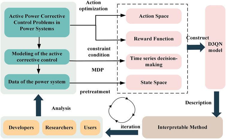
Figure 1. Machine learning model for active corrective control in power systems and its interpretable human-machine collaboration process.

3.2 D3QN model

Within the D3QN model, the reinforcement learning algorithm associates the present state with actions and rewards, guided by the anticipated return. The agent engages with the environment persistently, utilizing states, actions, and rewards to acquire knowledge through exploration and exploitation, culminating in the formulation of optimal decisions. The specific details are illustrated in Figure 2.

Figure 2

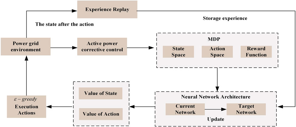
Figure 2. Logical framework of D3QN model for active power correction control in power systems.

In the D3QN model, states are no longer solely dependent on the value of actions for evaluation but can also undergo separate value predictions. The model can learn both the value of a particular state and the value of different actions in that state. It can independently and closely observe and learn the states and actions in the environment, allowing for more flexible handling.

$Q\left(s,a;\theta ,\alpha ,\beta \right)=V\left(s;\theta ,\beta \right)+A\left(s,a;\theta ,\alpha \right)(11)$

The D3QN network architecture incorporates two distinct branches following the convolutional network. V(s; θ, β) is employed to forecast the state’s value, while A(s, a; θ, α) is utilized to predict the value of actions associated with the state. Here, θ signifies the shared part of the network structure, and α and β represent the distinct parameters corresponding to these two branches. The outcomes from these two branches are subsequently combined to produce the Q-values.

In the overall D3QN algorithm workflow, the first step is to define the state space and action space. Then, two deep neural networks with essentially the same structure are established, including the current network θ_i and the target network ${{\theta }_i}^{\prime }$. These two networks consist of a shared convolutional layer and two branches: one for outputting state values V(s; θ, β) and the other for outputting advantage values for each action A(s, a; θ, α). Based on the present state and the Q-values output by the neural network, an action is chosen using a ɛ − greedy policy to maintain a certain level of algorithm exploration. The selected action is then executed, resulting in the next state and the corresponding reward. The states, actions, rewards, and next states [s_t, a_t, r_t, s_t+1] obtained during execution are stored in an experience pool for future training. Next, a batch of data is randomly selected from the experience pool for training the neural network. During the training process, mean squared error is used as the loss function to gradually approach the target Q-values with the network’s output Q-values.

3.3 The Deep-SHAP method

In current research, there are also studies that mention the adoption of feature importance interpretation methods for deep reinforcement learning (DRL) models Heuillet et al. (2022) Schreiber et al. (2022) Syavasya and Muddana (2022). In DRL, the aim of feature importance interpretation methods is to determine which input features are crucial for the model when making specific decisions. These methods typically calculate the importance of each input feature based on gradient information or changes in other model weights. For example, this paper mentions using backpropagation of gradients to compute the contribution of each input feature to the output, which aids in understanding which input features the model’s decisions are based on.

This paper proposes an interpretable feature importance method called Deep-SHAP, which combines traditional SHAP interpretable methods with backpropagation techniques. The specific algorithm framework is illustrated in Figure 3.

Figure 3

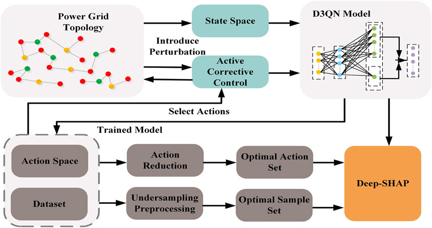
Figure 3. The Deep-SHAP algorithm framework for the D3QN model based on active corrective control.

Considering the long-tail effect in power grid data, where most of the time the system remains safe and stable, with only a few fault states, this paper preprocesses the state space S of the DRL model for active corrective control. The paper employs under-sampling techniques to randomly remove a portion of normal power grid state samples, with the objective of maximizing the purity of fault state samples, this paper introduces an objective function based on S to assess the information purity within the sample set. In particular, a smaller value of H corresponds to a higher purity level of S.

$\min H\left(S\right)=-{\displaystyle \sum _{d=1}^D}{p}_d{\log }_2{p}_d(12)$

where d represents the category of S, with d ∈ D, where D denotes the overall number of categories. The probability p_d denotes the likelihood that a sample belongs to the class d.

$\left\{\begin{array}{c}{s}_t\left[k\right]\in S_{f}failure\hfill \\ s_t\left[k\right]\in S_{n}else\hfill \end{array}\right.(13)$

where s_t[k] signifies the kth sample in the power grid state at the time instant t. The sets S_f and S_n respectively denote the sample sets containing faulty and normal power grid states. Following the binary classification of the samples, the objective is to obtain a sample set with the highest purity, specifically for the faulty samples of the power grid state.

$\begin{array}{ll}\hfill \min H\left(S\right)& =-\left(\left(P\left(S_f|S;\delta \right){\log }_2\left(P\left(S_f|S;\delta \right)+\left(P\left(S_n|S;\phi \right){\log }_2\right.\right.\right.\right.\hfill \\ \hfill & \times \left(P\left(S_n|S;\phi \right)\right)\hfill \end{array}(14)$

where δ and φ are the weights of S_f and S_n. Using the balanced sample set S′, the DEEP-SHAP explainability algorithm is employed to calculate the contribution values of model input features relative to the model’s output results.

$\begin{array}{ll}\hfill {\mathbf{x}}_i& =\left[x{\left(P_G,P_L,P_{TL},P_B,\rho \right)}_i^1,\cdots x{\left(P_G,P_L,P_{TL},P_B,\rho \right)}_i^k,\right.\hfill \\ \hfill & {\left.\cdots x{\left(P_G,P_L,P_{TL},P_B,\rho \right)}_i^K\right]}^T\hfill \end{array}(15)$

where xi denotes the set of features x_i across all input samples of the DRL model. The feature set in the state space encompasses the active power of generators, loads, transmission lines, buses, and the transmission line load ratios. $x{(P_G,P_L,PTL,P_B,\rho )}_i^k$ represents the ith feature in the kth sample, where i ∈ N_f, N_f denotes the total number of features, and K represents the sample count, where k is an element of the set K. The difference value $\mathrm{\Delta }{\mathbf{x}}_i^k$ between the load rate features $x_i^k$ and x_i in the sample space can be articulated as:

$\begin{array}{ll}\hfill \mathrm{\Delta }{\mathbf{x}}_i^k& =x_i^k-{\mathbf{x}}_i\hfill \\ \hfill & =\left[x{\left(P_G,P_L,P_{TL},P_B,\rho \right)}_i^k-x{\left(P_G,P_L,P_{TL},P_B,\rho \right)}_i^1,\cdots 0,\right.\hfill \\ \hfill & {\left.\cdots x{\left(P_G,P_L,P_{TL},P_B,\rho \right)}_i^k-x{\left(P_G,P_L,P_{TL},P_B,\rho \right)}_i^K\right]}^T\hfill \end{array}(16)$

Based on the DRL model, the action space includes actions for adjusting active power generator output and load shedding actions. The predicted output matrix of the model for the kth sample can be represented as follows:

${\mathbf{Y}}_k={\left[\begin{array}{ccccc}\hfill {\left(a_G,a_L\right)}_k^1\hfill & \hfill \cdots \hfill & \hfill {\left(a_G,a_L\right)}_k^h\hfill & \hfill \cdots \hfill & \hfill {\left(a_G,a_L\right)}_k^H\hfill \end{array}\right]}^T(17)$

where h stands for the hth action within the kth output action, where H denotes the total number of actions and h ∈ H.

Reinforcement learning models typically have large action spaces A. Therefore, for the DEEP-SHAP algorithm recommended in this manuscript, only the best output action $a_k^{h_{\mathit{opt}}}$ in the action space A specific to that sample is selected when calculating. By computing the reverse gradient of the model’s output, the optimal action decision $x_i^k$ with respect to any input feature can be obtained, resulting in the output differences under that input feature.

$\nabla f\left({\mathbf{x}}_i^k\right)=\frac{\partial a_k^{h_{\mathit{opt}}}}{\partial x{\left(P_G,P_L,P_{TL},P_B,\rho \right)}_i^k}(18)$

Leveraging reverse gradient calculation denotes the depiction of the influence of input features on the model’s output actions. This methodology facilitates the assessment of the marginal contribution value of features ${\mathbf{x}}_i^k$ to the optimal output action $a_k^{h_{\mathit{opt}}}$ for the kth sample.

$\begin{array}{ll}{C}_{\mathrm{\Delta }{x}_i^k\mathrm{\Delta }{a}_k^{h_{\mathit{opt}}}}\hfill & =\nabla f\left({\mathbf{x}}_i^k\right)\odot \mathrm{\Delta }{\mathbf{x}}_i^k\hfill \\ \hfill & =\frac{\partial a_k^{h_{\mathit{opt}}}}{\partial x{\left(P_G,P_L,P_{TL},P_B,\rho \right)}_i^k}\hfill & \odot \mathrm{\Delta }x{\left(P_G,P_L,P_{TL},P_B,\rho \right)}_i^k\hfill \end{array}(19)$

Through the Deep-SHAP interpretable algorithm, we can obtain a ranking of the contributions of input features to the model’s decision outcomes. The algorithmic logic of the DEEP-SHAP method is described in a more clear and intuitive manner in Algorithm 1.

Algorithm 1

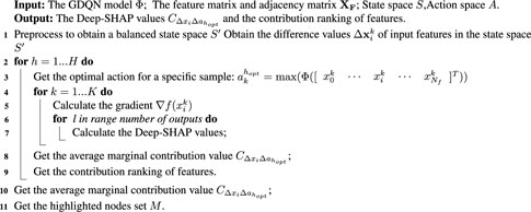
Algorithm 1. The distributed deep SHAP value method.

4 Cases study

4.1 A revised 36-bus system

In this study, we opted for an enhanced 36-bus system derived from the IEEE 118-bus system as our research setting. The schematic details of the power grid topology can be observed in Figure 4. This particular power grid system encompasses 36 substations, 59 transmission lines, 37 loads, 22 generators and 177 elements linked to the substations. The 36-bus system features various generator units, such as thermal, hydro, wind, solar, and nuclear power, with a substantial proportion dedicated to renewable energy installations. Our training environment is established using the Grid2Op open-source power system testing platform. Spanning 48 years of power grid data, the dataset for this power grid system accommodates scenarios over 28 consecutive days, accounting for fluctuations in supply and demand along with seasonal characteristics. Notably, all scenarios have been pre-scheduled to ensure power balance. Additionally, considering random disturbances in the system, each scenario experiences daily “N-1” line faults occurring at random times and locations. At the same time, planned outages for maintenance are also introduced in the test system. The goal of the agent is to perform time-based active corrective control in the 36-bus test system, eliminating and mitigating line overloads under “N-1” faults and supply-demand fluctuations to maintain stable system operation. The power flow calculation tool used in this case is LightSim2Grid.

Figure 4

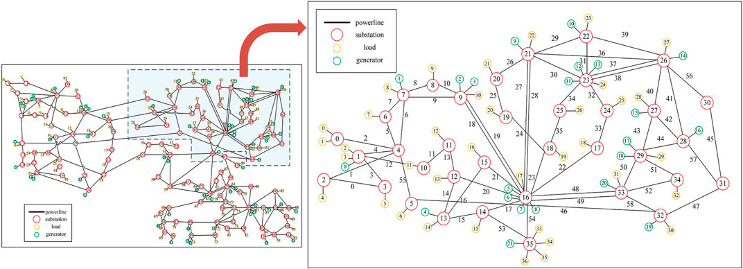
Figure 4. A revised 36-bus system derived from the IEEE 118-bus system.

In this case, the D3QN model is established based on the active corrective control objective. It considers using actions for adjusting generator active power output to eliminate and mitigate line overloads under “N-1” faults and supply-demand fluctuations. The decision cycle of the agent is 1 day, with a time interval of 5 min between t and t + 1 within a day. Therefore, under active corrective control, each scenario, in coordination with the scheduling plan, involves a sequential decision process comprising 288 decision steps within a day.

In the target power grid, there are a total of 177 components, including generators, loads, and the start and end points of transmission lines. In this paper, it is defined that each observable feature of each component falls into two types, including the transmission line load ratios and the active power of various components. The state space S characterizes the states observed by the agent within the power system, encompassing 354-dimensional features. The observed state of the components can be represented as:

${\mathbf{S}}_t={\left[\begin{array}{cccc}\hfill {\mathbf{X}}_1\left(P,\rho \right)\hfill & \hfill {\mathbf{X}}_2\left(P,\rho \right)\hfill & \hfill \cdots \hfill & \hfill {\mathbf{X}}_N\left(P,\rho \right)\hfill \end{array}\right]}^T(20)$

where X represents the observed feature vector on the components, and N is the number of components in the target power grid.

The action space A used in this paper consists of generator rescheduling actions. In this case, there are a total of 22 generators, including thermal, hydro, wind, solar, and nuclear power types. Among these, 10 generators are available for rescheduling adjustments. To simplify the action space, this paper stipulates that the action of generator rescheduling should consider a maximum of two simultaneously adjustable generators. Under the condition of considering only generator rescheduling actions, it is necessary to meet the power balance constraint. According to the reverse equal amount pairing principle, which means that the total sum of active power rescheduling of all generators is zero. This paper selects 1.4 MW, 2.8 MW, 4.3 MW, 8.5 MW, 9.9 MW, and 10.5 MW as various adjustment levels for generator rescheduling. For example, increasing the output of generator A by 2.8 MW while decreasing the output of generator B by 2.8 MW. Under this rule for adjusting active power of generators, there are a total of 153 possible actions to choose from, including the “do nothing” option.

4.2 Training and deployment of the D3QN model

Throughout the training of the D3QN model, significant attention is dedicated to addressing fluctuations in supply and demand as well as the inherent uncertainty associated with renewable energy sources. The training process encompasses 2,000 diverse scenarios, emulating a spectrum of operational conditions encountered in real power systems, including sudden shifts in load, generator failures, and faults in transmission lines. In each scenario, “N-1” line faults occur randomly, varying in both time and location. The agent’s task involves employing decision actions to regulate the active power output of generators within the power system to sustain stable operation. An assessment of the agent’s control effectiveness is based on the rewards garnered during the training process and the duration of time steps that the agent successfully navigates in each scenario. This evaluation is depicted in Figure 5.

Figure 5

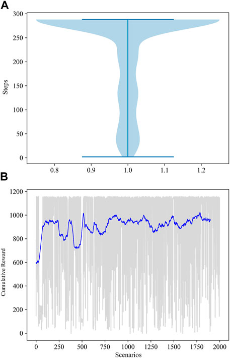
Figure 5. The reward accumulation trend throughout the agent’s training process, relative to the power system’s time progression. (A) Cumulative reward curve of the agent training process; (B) Distribution of system time step in different scenarios.

Figure 5B displays the cumulative reward curves associated with the agent throughout the training involving 2,000 scenarios, using a sliding average cumulative reward to facilitate better analysis. From Figure 5B, it can be observed that within the initial 750 training scenarios, the agent’s reward values were initially low and not very stable, exhibiting a trending but turbulent rise. However, after continuous training in the first 750 scenarios, the average cumulative reward curve becomes relatively stable. Figure 5B demonstrates the duration of time steps in which the D3QN agent is able to sustain system operation after encountering overload faults in the 2,000 training scenarios. Specifically, in a given scenario, when a random “N-1” event leads to overload faults in the system, if the agent’s decision actions cannot maintain the system’s continuous stable operation within three consecutive time steps, that scenario crashes, and the corresponding system operation steps stop. Figure 5A reveals that in the 2,000 training scenarios, after training in the initial 750 scenarios, the agent can run for more than 200 steps in 100% of the scenarios, and in 80% of the scenarios, it can achieve a complete operation duration of over 230 steps. The findings from this investigation suggest that the D3QN model is capable of guaranteeing the stability of the power system throughout a wide range of training scenarios, ensuring the sustained and uninterrupted normal functioning of the system.

After the agent completes its training, to further validate the deployment performance of the D3QN model, this section constructs a set of 500 test scenarios for the deployment and evaluation of the D3QN agent. To intuitively compare and verify that the D3QN model presented in this chapter can effectively address the issue of line overloads in active corrective control scenarios in the power system through generator rescheduling measures, this section provides two specific test scenarios for detailed analysis. Please refer to Table 1 for more details.

Table 1

Table 1. Details of the example scenario.

Figure 6A displays the line load rates before and after generator rescheduling in scenario 1. The blue and red lines represent the load rates before and after the adjustments, while the black line represents the load rate limit that the transmission lines can withstand. The horizontal axis represents the 59 transmission lines in the 36-bus system’s state space, and the vertical axis represents the load rate values on the transmission lines. It can be observed that, after the generator rescheduling actions proposed by the D3QN agent, the load rates on all transmission lines in the system are reduced to below 0.71. Figure 6B shows the load rate on the overloaded line during a complete cycle of 288 operating time steps. A random fault occurs at step 202, and after the agent takes decision actions, the overload issue on the 25th transmission line is resolved, and no further overload issues occur throughout the entire cycle. This indicates that the agent’s decision actions can reasonably address the system’s line overload issue, maintaining the system’s operational stability.

Figure 6

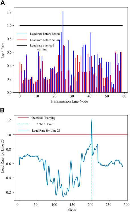
Figure 6. Transmission line load rate in test scenario 1. (A) Line load rates before and after generator rescheduling; (B) Line load rate within the system operation time step.

The specific details of scenario 2 are shown in Figure 7. Figure 7A displays the load rates on transmission lines before and after generator rescheduling. It can be observed that after the generator rescheduling, the load rates on all transmission lines in the system are reduced to below 0.8. In Figure 7B, the fault occurs at the 13th time step, and when the agent takes decision actions, the load rate on the 13th transmission line remains within a normal range throughout the entire cycle, and no further overloading issues occur. This indicates that the agent’s active corrective control decisions can effectively handle overloading fault situations.

Figure 7

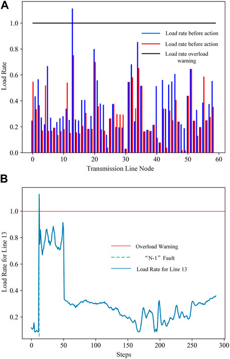
Figure 7. Transmission line load rate in test scenario 2. (A) Line load rates before and after generator rescheduling; (B) Line load rate within the system operation time step.

4.3 The Deep-SHAP method validation

To further validate the DEEP-SHAP method recommended in this manuscript in explaining the decision outcomes of DRL models in different scenarios, Figure 8 displays the sorting of the interpretable method’s impact on the agent model results by the significance of components. The vertical axis represents various equipment components in the power grid, arranged from top to bottom based on their contribution to the model’s output results. The horizontal axis represents the corresponding component’s SHAP value, which reflects the degree of contribution of the component to the model’s output results. The red area in the figure indicates a positive contribution to the decision outcomes of the model, while the blue area indicates a negative contribution to the decision outcomes of the DRL model.

Figure 8

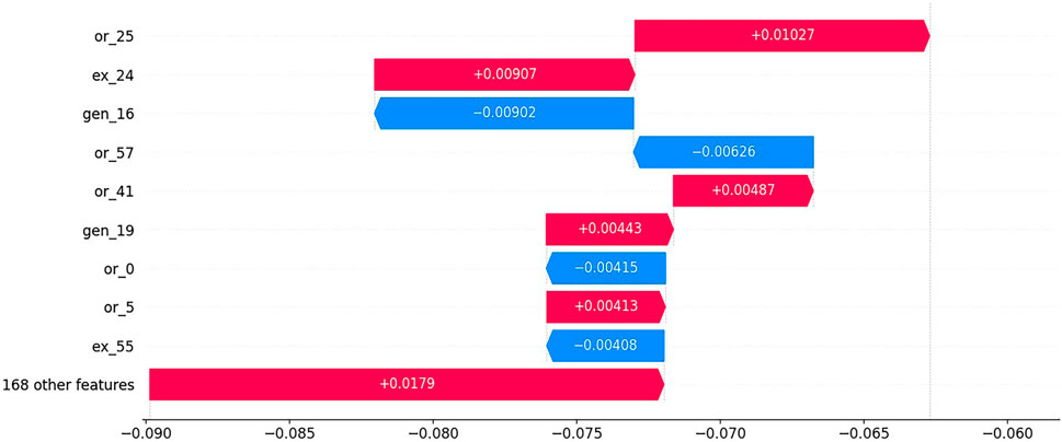
Figure 8. The explanation results of the DEEP-SHAP method in example scenario 1.

From Figure 8, it can be seen that the component with the most significant impact on the decision results of the D3QN model is transmission line 25. Following closely is transmission line 24. The results from the DEEP-SHAP interpretable method indicate that transmission line 24 has an important positive influence on the model’s output results. The load rate on transmission line 24 reaches 90%, indicating that it is overloaded. Similarly, component 41, which has a positive contribution, has a load rate of 89% on transmission line 41, indicating it is also overloaded. When dealing with overloaded lines, it is important to carefully consider the actions of adjacent generators. Increasing the active power output of generators adjacent to overloaded lines can significantly increase the load rate, potentially leading to the risk of overloading the line. Therefore, generator 16, which is connected to transmission line 41, needs special attention. At this time, generator 16 is in a standby state and, as shown in Figure 8, is having an inhibitory effect on the current decision results.

From Figure 8, it is evident that the factors significantly impacting the decision-making results of the intelligent agent are mainly concentrated on heavily loaded or overloaded transmission lines, as well as generators with abnormal output states. Model interpretation methods, such as feature importance, are usually helpful for grid dispatchers to better understand the current status of the power system. For reinforcement learning agents, decision-making results are directly reflected in the reward function. In the active power correction control task proposed for our 36-node system, the reward function mainly involves penalties for overloaded and heavily loaded transmission lines. Therefore, the performance of feature importance is more reflected in the transmission lines that are overloaded or heavily loaded. To better understand the relationship between the active power output states of components that significantly contribute to the system and the line load ratio states, Table 2 provides detailed information on the top 5 components with higher contributions as shown in Figure 8 by the Deep-SHAP method, including their SHAP values and probability representations.

Table 2

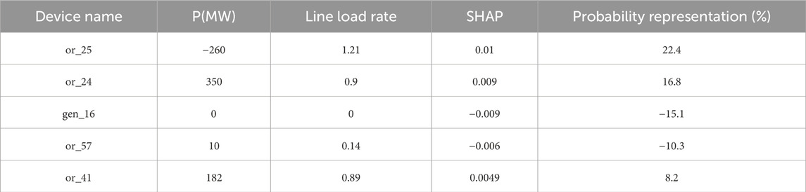
Table 2. The value about the top five important components in example scenario 1

In the case of example scenario 2, Figure 9 provides a ranking of components with a relatively larger influence on the intelligent agent’s model results, as obtained through the DEEP-SHAP method. Among the components shown in Figure 9, transmission lines 13 and 11 have a significant positive impact. Transmission line 13 is overloaded, and line 11 has a load rate of 97%, indicating it is heavily loaded. Information about these overloaded lines is crucial for decision-making by the grid operator. Additionally, generator 16 and generator 19 are identified as components that require special attention. Generator 16 currently has an active power output of 0, indicating it is in standby mode and may need to be considered for increasing its active power output. Generator 19 has an active power output of 400 MW, which is at its upper limit, making it another key element for the grid operator to monitor closely. Figure 9 also highlights the positive contribution of load 27 to decision-making actions. You can observe that load 27 currently consumes 122 MW of active power, making it one of the larger consumers of active power in the target network.

Figure 9

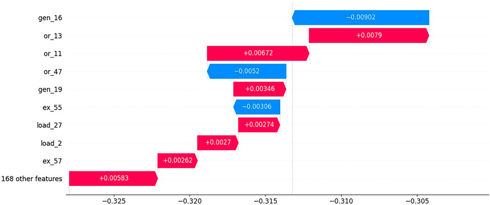
Figure 9. The explanation results of the DEEP-SHAP method in example scenario 2.

In the context of Scenario 2, as clearly observed from Figure 9, the factors significantly impacting the decision outcomes of the intelligent agent are primarily concentrated in the overloaded and overburdened transmission lines, as well as the abnormal output states of the generator. Table 3 provides detailed information on the top five components, obtained through the Deep-SHAP method, that exert a greater influence on the intelligent agent model results. This information includes their SHAP values and probability representations.

Table 3

Table 3. The value about the top five important components in example scenario 2

Through the specific sample analysis of these two test scenarios, it can be observed that the interpretable results of the D3QN model’s decisions help operators understand the reasons behind the intelligent agent’s decision-making. It is crucial to emphasize that SHAP values can reveal relationships between input features and output outcomes learned from the data, they do not inherently signify or mirror causality. Consequently, operators or domain experts should undertake additional verification using domain knowledge or alternative causal reasoning methods to ascertain the causal effects of the interpretable approach Hamilton and Papadopoulos (2023).

This article supplements the comparison between the proposed Deep-SHAP method and the traditional SHAP value method. The specific content is as follows:

To validate the superiority of the Deep-SHAP interpretable method proposed in this paper over the initial SHAP method in terms of computational efficiency, a comparison of the two methods is presented, as shown in Table 4.

Table 4

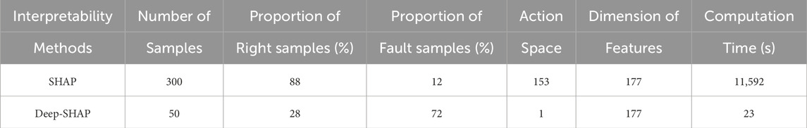
Table 4. Comparison between Deep-SHAP and SHAP methods.

Considering the issue of computational complexity, this study randomly selected 300 scenarios from a 36-node system to construct the initial sample set. Table 4 shows that the fault samples account for 12% of the initial sample set, the action space contains 153 actions, and the dimension of the model input features is 177. In this scenario, the SHAP method requires 11,592 s of computation time, which is impractical for power system correction control. Therefore, the SHAP interpretable method cannot be applied to the decision explanation of the correction control deep reinforcement learning model. In the Deep-SHAP interpretable method, sample selection is performed from the initial sample set through undersampling techniques to increase the proportion of fault samples. At this point, the sample set contains 50 samples, with fault samples accounting for 72% of the total sample set. By selecting actions, only the most likely predicted actions are retained. In this case, the computational time cost of the Deep-SHAP interpretable method is 23 s, which is 504 times more efficient compared to the SHAP method. This validates the superiority of the Deep-SHAP method proposed in this paper in terms of computational efficiency.

This paper further considers the accuracy of the interpretability of the two methods on a single sample and conducts a comparative analysis. For the SHAP and Deep-SHAP interpretable methods computed in Table 4, this study randomly selects 100 samples to compare the features that are significantly contributing to the model results according to the two methods, and performs an accuracy analysis, as shown in Figure 10 and Figure 11, and Table 5. Using the output feature importance results of the SHAP method as the baseline, this paper compares the accuracy of the output feature importance under the Deep-SHAP method in Figure 10 and reveals the distribution range of feature importance accuracy in Figure 11.

Figure 10

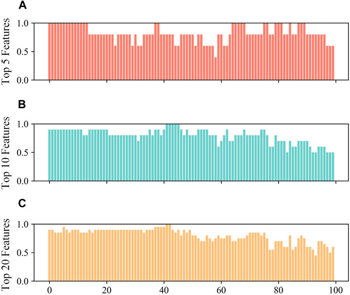
Figure 10. The comparison of the accuracy of the Deep-SHAP method and the SHAP method on a single sample. (A): accuracy of top 5 features. (B): accuracy of top 10 features. (C): accuracy of top 20 features.

Figure 11

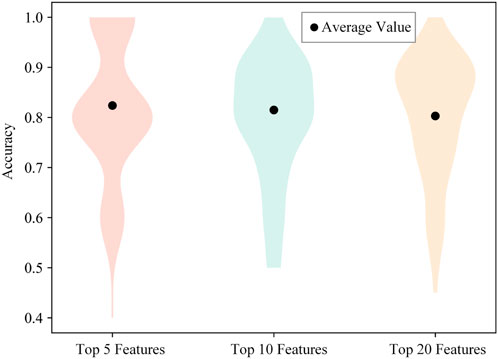
Figure 11. The accuracy distribution of the Deep-SHAP method compared to the SHAP method on a single sample.

Table 5

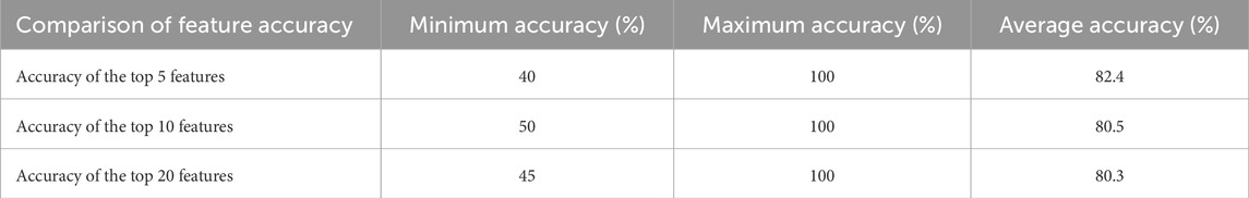
Table 5. Comparison of accuracy between the Deep-SHAP and SHAP methods on individual samples.

Figure 10A shows the accuracy percentages of the top 5 features for 100 samples under the Deep-SHAP method, with a minimum of 40% and a maximum of 100%, and an average accuracy of 82.4%. Figure 10B displays the accuracy percentages of the top 10 features for 100 samples under the Deep-SHAP method, with a minimum of 50%, a maximum of 100%, and an average accuracy of 80.5%. Figure 10C presents the accuracy percentages of the top 20 features for 100 samples under the Deep-SHAP method, with a minimum of 45%, a maximum of 100%, and an average accuracy of 80.3%. Figure 2 indicates that, compared to the SHAP method, the Deep-SHAP method maintains an average accuracy of over 80%. These results, which show highly similar outcomes between the two methods, demonstrate that the Deep-SHAP method proposed in this paper can effectively replace the interpretability results of the SHAP method while significantly improving computational efficiency.

5 Conclusion

This paper proposes the use of an improved 36-bus system as a representative task scenario, completing the training and deployment tasks for the D3QN agent. Through the analysis of the agent’s reward curve during the training process and the duration of system survival, the effectiveness of the D3QN agent in active corrective control is verified. Additionally, this paper validates the proposed DEEP-SHAP interpretable method on the improved 36-bus system, which enhances the transparency and reliability of the active corrective D3QN model. Through the analysis of specific scenario examples, operators can understand the contribution of model input features to output decisions, and by combining experience and domain knowledge, operators can grasp causality relationships. This improves the trust and acceptance of operators in the DRL model for active corrective control presented in this paper.

Data availability statement

The original contributions presented in the study are included in the article/Supplementary material, further inquiries can be directed to the corresponding author.

Author contributions

BL: Writing–original draft, Writing–review and editing, Conceptualization, Formal Analysis, Methodology, Project administration, Resources, Validation. QL: Methodology, Project administration, Supervision, Funding acquisition, Investigation, Resources, Validation, Visualization, Writing–review and editing. YH: Conceptualization, Data curation, Formal Analysis, Investigation, Methodology, Project administration, Supervision, Writing–review and editing. YH: Conceptualization, Data curation, Formal Analysis, Investigation, Methodology, Writing–review and editing. LZ: Conceptualization, Data curation, Formal Analysis, Investigation, Methodology, Visualization, Writing–original draft. ZH: Data curation, Formal Analysis, Methodology, Project administration, Resources, Visualization, Writing–original draft. XF: Data curation, Formal Analysis, Investigation, Methodology, Project administration, Resources, Writing–review and editing. TG: Conceptualization, Formal Analysis, Methodology, Project administration, Resources, Supervision, Validation, Visualization, Writing–original draft. LY: Conceptualization, Data curation, Investigation, Methodology, Project administration, Resources, Writing–review and editing.

Funding

The author(s) declare that no financial support was received for the research, authorship, and/or publication of this article.

Conflict of interest

Authors BL, QL, YH, YH, LZ, ZH, XF, and LY were employed by State Grid Hubei Electric Power Company.

The remaining authors declare that the research was conducted in the absence of any commercial or financial relationships that could be construed as a potential conflict of interest.

Publisher’s note

All claims expressed in this article are solely those of the authors and do not necessarily represent those of their affiliated organizations, or those of the publisher, the editors and the reviewers. Any product that may be evaluated in this article, or claim that may be made by its manufacturer, is not guaranteed or endorsed by the publisher.

References

Fitzmaurice, R., Keane, A., and O’Malley, M. (2010). Effect of short-term risk-aversive dispatch on a complex system model for power systems. IEEE Trans. Power Syst. 26, 460–469. doi:10.1109/tpwrs.2010.2050079

CrossRef Full Text | Google Scholar

Hamilton, R. I., and Papadopoulos, P. N. (2023). Using shap values and machine learning to understand trends in the transient stability limit. IEEE Trans. Power Syst. 39, 1384–1397. doi:10.1109/tpwrs.2023.3248941

CrossRef Full Text | Google Scholar

Heuillet, A., Couthouis, F., and Diaz-Rodriguez, N. (2022). Collective eXplainable AI: explaining cooperative strategies and agent contribution in multiagent reinforcement learning with shapley values. IEEE Comput. Intell. Mag. 17, 59–71. doi:10.1109/mci.2021.3129959

CrossRef Full Text | Google Scholar

Hossain, R. R., Huang, Q., and Huang, R. (2021). Graph convolutional network-based topology embedded deep reinforcement learning for voltage stability control. IEEE Trans. Power Syst. 36, 4848–4851. doi:10.1109/tpwrs.2021.3084469

CrossRef Full Text | Google Scholar

Kim, B., Khanna, R., and Koyejo, O. (2016). Examples are not enough, learn to criticize! Criticism for interpretability. Adv. Neural Inf. Process. Syst. (Barcelona, Spain), 2288–2296.

Google Scholar

Liu, F., Wang, X., Li, T., Huang, M., Hu, T., Wen, Y., et al. (2023). An automated and interpretable machine learning scheme for power system transient stability assessment. Energies 16, 1956. doi:10.3390/en16041956

CrossRef Full Text | Google Scholar

Mitrentsis, G., and Lens, H. (2022). An interpretable probabilistic model for short-term solar power forecasting using natural gradient boosting. Appl. Energy 309, 118473. doi:10.1016/j.apenergy.2021.118473

CrossRef Full Text | Google Scholar

Molnar, C. (2020). Interpretable machine learning. North Carolina, United States: lulu.com.

Google Scholar

Ren, J., Li, B., Zhao, M., Shi, H., You, H., and Chen, J. (2021). Optimization for data-driven preventive control using model interpretation and augmented dataset. Energies 14, 3430. doi:10.3390/en14123430

CrossRef Full Text | Google Scholar

Schreiber, L. V., Alegre, L. N., Bazzan, A. L., De, O., and Ramos, G. (2022). “On the explainability and expressiveness of function approximation methods in RL-based traffic signal control,” in Proceedings of the international joint Conference on neural networks (padua, Italy), 2022. doi:10.1109/ijcnn55064.2022.9892422

CrossRef Full Text | Google Scholar

Shrikumar, A., Greenside, P., and Kundaje, A. (2017). “Learning important features through propagating activation differences,” in International conference on machine learning (PMLR), 3145–3153.

Google Scholar

Syavasya, C., and Muddana, A. L. (2022). Optimization of autonomous vehicle speed control mechanisms using hybrid DDPG-SHAP-DRL-stochastic algorithm. Adv. Eng. Softw. 173, 103245. doi:10.1016/j.advengsoft.2022.103245

CrossRef Full Text | Google Scholar

Wang, Z., Liu, F., Low, S. H., Zhao, C., and Mei, S. (2019). Distributed frequency control with operational constraints, Part I: per-node power balance. IEEE Trans. Smart Grid 10, 40–52. doi:10.1109/tsg.2017.2731810

CrossRef Full Text | Google Scholar

Wu, B., Wang, L., and Zeng, Y.-R. (2022). Interpretable wind speed prediction with multivariate time series and temporal fusion transformers. Energy 252, 123990. doi:10.1016/j.energy.2022.123990

CrossRef Full Text | Google Scholar

Xu, H., Yu, Z., Zheng, Q., Hou, J., Wei, Y., and Zhang, Z. (2019). Deep reinforcement learning-based tie-line power adjustment method for power system operation state calculation. IEEE Access 7, 156160–156174. doi:10.1109/access.2019.2949480

CrossRef Full Text | Google Scholar

Xu, P., Duan, J., Zhang, J., Pei, Y., Shi, D., Wang, Z., et al. (2021). Active power correction strategies based on deep reinforcement learning—part i: a simulation-driven solution for robustness. CSEE J. Power Energy Syst. 8, 1122–1133. doi:10.17775/CSEEJPES.2020.07090

CrossRef Full Text | Google Scholar

Yang, Y., Huang, Q., and Li, P. (2022). Online prediction and correction control of static voltage stability index based on Broad Learning System. Expert Syst. Appl. 199, 117184. doi:10.1016/j.eswa.2022.117184

CrossRef Full Text | Google Scholar

Zhang, C., Liu, Q., Zhou, B., Chung, C. Y., Li, J., Zhu, L., et al. (2023a). A central limit theorem-based method for DC and AC power flow analysis under interval uncertainty of renewable power generation. IEEE Trans. Sustain. Energy 14, 563–575. doi:10.1109/tste.2022.3220567

CrossRef Full Text | Google Scholar

Zhang, K., Xu, P., Gao, T., and Zhang, J. (2021). “A trustworthy framework of artificial intelligence for power grid dispatching systems,” in 2021 IEEE 1st international conference on digital twins and parallel intelligence (DTPI) (IEEE), 418–421.

CrossRef Full Text | Google Scholar

Zhang, K., Zhang, J., Xu, P., Gao, T., and Gao, W. (2023b). A multi-hierarchical interpretable method for drl-based dispatching control in power systems. Int. J. Electr. Power & Energy Syst. 152, 109240. doi:10.1016/j.ijepes.2023.109240

CrossRef Full Text | Google Scholar

Zhang, R., Yao, W., Shi, Z., Zeng, L., Tang, Y., and Wen, J. (2022). A graph attention networks-based model to distinguish the transient rotor angle instability and short-term voltage instability in power systems. Int. J. Electr. Power & Energy Syst. 137, 107783. doi:10.1016/j.ijepes.2021.107783

CrossRef Full Text | Google Scholar

Zhang, Z., Zhang, D., and Qiu, R. C. (2019). Deep reinforcement learning for power system applications: an overview. CSEE J. Power Energy Syst. 6, 213–225. doi:10.17775/CSEEJPES.2019.00920

CrossRef Full Text | Google Scholar

Zheng, X., Khodayar, M. E., Wang, J., Yue, M., and Zhou, A. (2024). Distributionally robust multistage dispatch with discrete recourse of energy storage systems. IEEE Trans. Power Syst., 1–14. doi:10.1109/tpwrs.2024.3369664

CrossRef Full Text | Google Scholar