Coordinated energy storage and network expansion planning considering the trustworthiness of demand-side response

The enhancement of economic sustainability and the reduction of greenhouse gas (GHG) emissions are becoming more relevant in power system planning. Thus, renewable energy sources (RESs) have been widely used as clean energy for their lower generation costs and environmentally friendly characteristics. However, the strong random uncertainties from both the demand and generation sides make planning an economic, reliable, and ecological power system more complicated. Thus, this paper considers a variety of resources and technologies and presents a coordinated planning model including energy storage systems (ESSs) and grid network expansion, considering the trustworthiness of demand-side response (DR). First, the size of a single ESS was considered as its size has a close effect on maintenance costs and ultimately affects the total operating cost of the system. Second, it evaluates the influence of the trustworthiness of DR. Third, multiple resources and technologies were included in this high-penetration renewable energy integrated power system, such as ESSs, networks, DR technology, and GHG reduction technology. Finally, this model optimizes the decision variables such as the single size and location of ESSs and the operation parameters such as thermal generation costs, loss load costs, renewable energy curtailment costs, and GHG emission costs. Since the problem scale is very large not only due to the presence of various devices but also both binary and continuous variables considered simultaneously, we reformulate this model by decomposition. Then, we transform it into a master problem (MP) and a dual sub-problem (SP). Finally, the proposed method is applied to a modified IEEE 24-bus test system. The results show computational effectiveness and provide a helpful method in planning low-carbon electricity power systems.

1 Introduction

The fuels used to power conventional power plants cause unsustainable and environmentally unfriendly impacts, especially during peak load-carrying hours and critical weather conditions. Therefore, the global common goal is to mitigate dependence on fossil fuels and reduce greenhouse gas (GHG) emissions. Renewable energy sources (RESs) (wind and photovoltaic power are the leading alternatives) have become the main focus of many recent energy policies (Paris agreement, 2015; Summary for policymakers, 2021). According to the Energy Roadmap 2050 (European Commission and Energy Roadmap, 2050, 2011), the European Commission is moving toward a low GHG emission economic entity. Under this blueprint, the de-carbonization target will be possible with an even higher RES penetration level (Zappa et al., 2019). However, higher RES penetration faces greater volatility, resulting in the power grids having more fragile, less flexible, and low reliable characteristics. Then, under the circumstance of multiple resources and technologies, how to get a more flexible, reliable, environmentally friendly, and cost-efficient power system has gained increasing attention (Al-Shetwi, 2022). This paper presents a coordinated planning model for a high-penetration renewable energy integrated power system including energy storage systems (ESSs) and network expansion, considering the trustworthiness of DR).

To cope with fundamental challenges, a vast range of literature focuses on DR and its effects on the optimal performance of power grids. Qi et al. (2021) proposed a smart energy hub in which an analytical framework containing several DR programs is adopted. Results show that DR has a positive impact on long-term resource planning. Mansouri et al. (2022) showed a two-stage stochastic model based on DR and integrated DR programs. Many uncertainties are included in this model, such as electrical, heating, cooling loads, and the wind turbine’s output power. According to Aghajani et al. (2017), with the consideration of suitable DR, the uncertainties caused by wind and photovoltaic power can be handled appropriately. Thus, optimal operation optimization to decrease costs and minimize GHG emissions has been presented. In a word, appropriate DR in a smart grid helps resist volatility. However, the trustworthiness of DR has a deep internal influence on power system planning, which is seldom included and needs to be further studied in the future.

Previous studies (Liu et al., 2018; Zhang et al., 2020; Jafari et al., 2022; Liu et al., 2022) focused on optimally utilizing novel resources or technologies to respond to any uncertain variation (it usually comes from RESs, demand, and equipment failures). It is well known that installing ESSs may enhance power system flexibility by providing higher ramp rates or ramp ranges for power grids. Therefore, fast-response ESSs are considered promising resources. Li Z. et al. (2021) applied a bilayer model with heterogeneous ESSs to alleviate the adverse effects of diverse uncertainties and obtain the economic multi-energy building microgrid operation. Ramos-Real et al. (2018) followed another approach to obtain a promising alternative from an economic and environmental perspective through a high deployment of RESs and ESSs in the Canary Islands. Shi et al. (2022) proposed a hierarchical optimization planning model, with its objective function including the cost of ESSs and renewable energy. To minimize the system’s total expected cost, voltage deviation, and power loss mitigation, ALAhmad (2023) proposed a novel probabilistic optimization model by optimally placing and sizing ESSs to alleviate the negative impact of the high penetration of RESs and enhance grid stability.

Based on the above literature, the flexibility and reliability that ESSs brought to the system were expounded. However, how to effectively incorporate these ESSs into the power grids still needs to be investigated. Li et al. (2023) proposed a bi-level optimization model to minimize net load fluctuation, voltage deviation, and total costs by determining the optimal location, power rating, capacity, and hourly charging/discharging profile in a multiple-ESS-containing system. Jiang et al. (2020) simultaneously considered the location, capacity, and power rating of ESSs. The optimal deployment of ESSs provided benefits such as power curtailment reduction, power loss mitigation, and arbitrage profit maximization. Li J. et al. (2021) proposed a bi-level optimization problem that was decomposed by the decomposition–coordination algorithm into two sub-systems. The model determines the optimal location, power rating, and capacity of ESSs to maximize the system’s net profit and minimize the system’s total operation cost. Li Z. et al. (2020) presented a risk-averse method for heterogeneous ESS deployment in a residential multi-energy microgrid where a multistage adaptive stochastic optimization approach is utilized to deal with various uncertainties. However, these existing research studies have not fully addressed the single size, location, and degradation of ESSs simultaneously, all of which have a true existence in practical applications. Moreover, because of the geographical and labor management issues, the size of a single ESS will closely affect its maintenance costs and ultimately affect the total operating cost of the system. Thus, the optimal single size, location, and operation of ESSs to enhance system flexibility and reduce GHG emissions in power grids is an important ongoing research area that is worthy of further study.

Although there have been many researchers working on investigating the influence of multiple resources and technologies in photovoltaic or wind-integrated power systems, the need for comprehensive research considering not only ESSs and DR but also further CO₂ reduction still remains. Many carbon financing policies (e.g., carbon emission tax and building committed carbon emission operation regions) have been proven to be exceedingly effective methods to encourage participators toward emission reduction. For instance, carbon emission tax is utilized in Olsen et al. (2018) for achieving emission targets in the electricity market. Jiang et al. (2024) proposed the committed carbon emission operation region to characterize the low-carbon feasible space. Results show that it can achieve integrated energy system decarbonization. Hu et al. (2024) presented a bi-level carbon-oriented planning method containing shared ESSs for integrated energy systems. Simulation results show that it is more environmentally friendly and economical compared to the model without shared ESSs. Cheng et al. (2019) proposed a bi-level multi-energy system planning model, in which carbon emission flow was included. These decentralized approaches are employed to calculate the emission amount but fail to involve active DR simultaneously.

According to all the above, countries all around the world are pursuing a low-carbon power system to achieve sustainable development. Achieving this requires the coordination of a variety of electricity technologies. First, the vast emergence of RESs provides alternative generations, while traditional coal-fired generations are being phased out. However, high RES penetration causes huge challenges in the stability of voltage, frequency, and the balance between supply and demand. Second, various forms of ESSs, including electrochemical ESSs, are regarded as important sources that cut the peaks and fill the valleys to provide flexibility effectively. However, their size, location, and inherent degradation should be considered in the planning stage. Third, DR, as an active response on the demand side, helps resist system volatility. However, few researchers consider the trustworthiness of DR and reveal their deep internal impact on the system. Moreover, these latest technologies are usually expensive and eco-friendly in the early stages, which is contrary to the goal of minimizing total costs. However, the control of carbon emissions is the basis of sustainable development. Thus, this contradictory factor needs to be considered in the planning stage. In a word, this paper aims to provide a more practical method for power system planning under the background of a high proportion of renewable energy by comprehensively utilizing various types of latest technologies and taking carbon reduction into account. The comparison with related studies is presented in Table 1.

Table 1

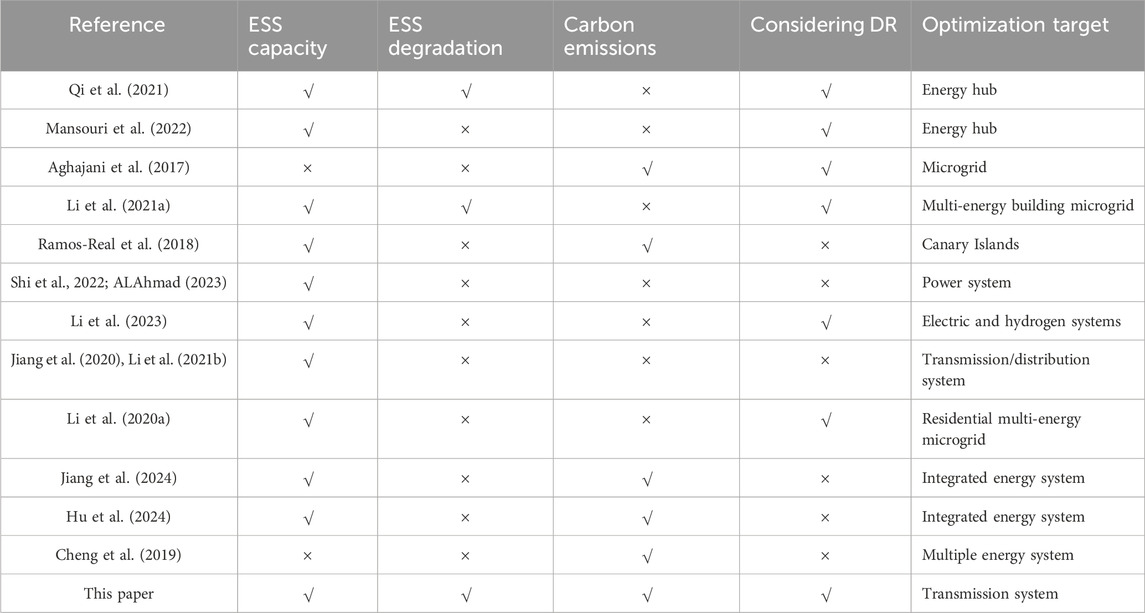
Table 1. Comparison between the proposed model of this work and previous studies.

In response, we aim to bridge the gaps mentioned above and propose a novel model that optimizes local network reinforcement along with investment decisions on ESSs. The size, location, and degradation of ESSs and the trustworthiness of DR technology are included because they represent some promising options to provide flexibility in power grids. In addition, the presented expansion approach takes conventional generation costs, investment costs (including ESSs and transmission lines), loss load costs, energy curtailment costs, and GHG emission costs into account. However, the problem scale is very large not only due to various devices but also both binary and continuous variables considered simultaneously. To deal with this, we reformulate this model by decomposition and transform it into an MP and a dual SP. Then, it can be solved efficiently without falling into a poor, sub-optimal solution. Using this new framework, power systems can take a comprehensive methodology to better handle the inherent resources to get a more flexible, reliable, environmentally friendly, and cost-efficient power system. The proposed solution technique is tested in a modified 24-bus system. The results show the superiority of this method in terms of solution optimality and computational efficiency. To sum up, this model can help all agents who participate in power grids make their cost-effective plans in a carbon-constrained environment.

The main contributions of this paper are as follows:

1. To evaluate what the influences of multiple resources and technologies that act on power system planning are, we proposed a coordinated planning model that considers not only the effects of ESSs but also the trustworthiness of DR and CO₂ emissions.

2. Moreover, the size, location, and degradation of ESSs are included in this model and reveal how the deep internal influence of different trustworthiness of DR acts on power grids.

3. Our model can comprehensively investigate the goals between environmental benefits and cost-effectiveness. Thus, it can provide guidance for policymakers on how to formulate policy interventions for participants to achieve emission targets.

4. This framework was decomposed by the dual theory to reduce the computational burden without falling into a poor, sub-optimal solution.

The remainder of this paper is organized as follows: the detailed mathematical model is formulated in Section 2. Its compact vector form and its dual decomposition are presented in Section 3. Section 4 introduces the overall solution structure. The performance of the presented method is evaluated on a modified IEEE 24-bus test system, which is shown in Section 5. Finally, the main conclusions are summarized in Section 6.

2 Problem formulation

This section introduces the research framework and modeling process of this article. As shown in Figure 1, to consider the environmental, economic, and reliability factors simultaneously during the planning phase, we conducted a planning study on a power system with a high penetration rate of renewable energy. First, coal-fired power plants emit GHGs, which may be advantageous for maximizing economic benefits but detrimental to the current sustainable development purport. This contradictory factor needs to be considered in the planning stage. Second, ESSs can perform peak shaving and valley filling and provide flexibility to the system. However, their size, location, and inherent degradation should be considered in the planning stage. Finally, DR, as an active response on the demand side, helps resist system volatility. However, the trustworthiness of DR is influenced by various factors and can ultimately affect the planning results of this system. Thus, this article presents a more practical method for power system planning from ecological, economic, and reliability perspectives with a high penetration rate of renewable energy.

Figure 1

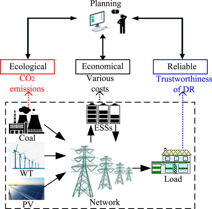
Figure 1. Framework of this article

2.1 Objective function

The objective function shown in Equation 1 (which contains four parts) seeks to make a tradeoff between minimizing the costs and CO₂ emissions. The first part refers to the total investment costs of new transmission lines and ESSs, which is indicated in Equation 2; the second part refers to the total operation costs, including conventional generation costs ($P{G}^{ope}$), ESSs maintenance costs ($P{S}^{ope}$), DR costs ($D{R}^{ope}$), and renewable energy curtailment costs ($QW{V}^{ope}$). The details of these compact forms are shown in Equations 4–7. It should be noted that the maintenance costs of per-unit ESSs decrease as their node-installed capacity increases. The third part ($C^{reli}$), as indicated in Equation 8, refers to the total costs of loss of demands. The last part ($C^{em}$) that is shown in Equation 9 is GHG emission costs for every time point in every representative day. If environmental considerations are not taken into account, the objective function only contains the first three costs. Note that GHG emission cost is closely related to traditional generations, which is shown in Equation 10 in detail.

$\min C^{inv}+C^{ope}+C^{reli}+C^{em},(1)$

$C^{inv}=\frac{r{\left(1+r\right)}^y}{{\left(1+r\right)}^y-1}\left[{\displaystyle \sum _i}C{L}_i\cdot x{l}_i+{\displaystyle \sum _s}C{S}_s\cdot x{s}_s\right],(2)$

$C^{ope}={\displaystyle \sum _k}{\rho }_k\cdot {\displaystyle \sum _{y,h}}\cdot \left[P{G}^{ope}+P{S}^{ope}+D{R}^{ope}+QW{V}^{ope}\right],(3)$

$P{G}^{ope}={\displaystyle \sum _g}{\alpha }_{g,y,h}\cdot P{G}_{g,y,h,k},(4)$

$P{S}^{ope}={\displaystyle \sum _s}\left({\beta }_{y,h}-\frac{E_{y,h}-{E_0}_{,y,h}}{E_{y,h}}*\hslash \right)\cdot E_{y,h},(5)$

$D{R}^{ope}=-{\displaystyle \sum _l}{\gamma }_{y,h}\cdot D{R}_{l,y,h,k},(6)$

$QW{V}^{ope}={\displaystyle \sum _w}C{W}_{w,h}\cdot Q{W}_{w,y,h,k}+{\displaystyle \sum _v}C{V}_{v,h}\cdot Q{V}_{v,y,h,k},(7)$

$C^{reli}=VOLL\cdot {\displaystyle \sum _{i,y,h,k}}{\rho }_k\cdot L{P}_{i,y,h,k},(8)$

$C^{em}={\displaystyle \sum _k}{\rho }_k\cdot {\displaystyle \sum _{g,y,h}}E{M}_{g,y,h}\cdot C{G}_{g,y,h}^{em}\cdot e_{g,y,h,k},(9)$

$e_{g,y,h,k}=P{G}_{g,y,h,k}·h,\forall g,y,h,k.(10)$

2.2 Constraints

Various expansion and operation constraints are presented as follows:

The constraints of Equations 11–15 are introduced for conventional generators’ operation limits. Considering the upward and downward reserve, constraints of Equations 11, 12 limit the active power production of each conventional generator between its minimum and maximum capacities. The ramp-up and ramp-down limits of traditional generator units are shown in Equations 13, 14. In Equation 15, the reactive power production was limited.

$P{G}_{g,y,h,k}+R{U}_{g,y,h,k}\le P{G}_g^{\max },\forall g,y,h,k,(11)$

$R{D}_{g,y,h,k}\le P{G}_g^{\min },\forall g,y,h,k,(12)$

$P{G}_{g,y,h,k}-P{G}_{g,y,h-1,k}+R{U}_{g,y,h,k}\le RU{W}_g,\forall g,y,h,k,(13)$

$P{G}_{g,y,h-1,k}-P{G}_{g,y,h,k}+R{D}_{g,y,h,k}\le RD{W}_g,\forall g,y,h,k,(14)$

$Q{G}_g^{\min }\le Q{G}_{g,y,h,k}\le Q{G}_g^{\max },\forall g,y,h,k.(15)$

The upward and downward spinning reserves are modeled to resist the inevitable uncertainties due to renewable energy and demand, which are bounded from Equations 16–19. $W{f}_h$ and $V{f}_h$ are the hourly representative factors of the wind and photovoltaic farms' output. It affects the final output of these generations. Load forecasting is almost patterned, and its prediction is relatively easy. However, the trustworthiness of DR is complicated because it is affected by several factors. Moreover, as RESs are highly penetrated, their outputs are affected by the weather, causing larger forecast errors. Thus, we assume the lower bound for the upward and downward spinning reserves at every time resolution as 3% for the load and 5% for renewable energy (see in Equations 16, 17). The hourly total upper bounds of the upward and downward reserves are presented in Equations 18, 19.

$3\%\cdot {\left(1+L{G}_k\right)}^k\cdot {\displaystyle \sum _h}L{f}_h\cdot P{D}_{i,k}^{PK}+5\%\cdot \left({\displaystyle \sum _h}W{f}_h\cdot {\displaystyle \sum _{w,k}}P{W}_{w,k}+{\displaystyle \sum _h}V{f}_h\cdot {\displaystyle \sum _{v,k}}P{V}_{v,k}\right)\le {\displaystyle \sum _{g,h}}R{U}_{g,y,h,k},\forall y,k,(16)$

$3\%\cdot {\left(1+L{G}_k\right)}^k\cdot {\displaystyle \sum _h}L{f}_h\cdot P{D}_{i,k}^{PK}+5\%\cdot \left({\displaystyle \sum _h}W{f}_h\cdot {\displaystyle \sum _{w,k}}P{W}_{w,k}+{\displaystyle \sum _h}V{f}_h\cdot {\displaystyle \sum _{v,k}}P{V}_{v,k}\right)\le {\displaystyle \sum _{g,h}}R{D}_{g,y,h,k},\forall y,k,(17)$

${\displaystyle \sum _{g,h}}R{U}_{g,y,h,k}\le RU{W}_g,\forall g,y,h,k,(18)$

${\displaystyle \sum _{g,h}}R{D}_{g,y,h,k}\le RD{W}_g,\forall g,y,h,k.(19)$

Constraints related to renewable energy are presented in Equations 20–22. Constraints of Equations 20, 21 limit the power production of RESs (including wind farms and photovoltaic generations) from zero to their maximum capacity. The constraint of Equation 22 ensures the penetration of renewable energy; in other words, it guarantees the percentage of the total load supplied by renewable energy. The parameter $\chi$ represents the expected contributions of RESs in supplying the total demand.

$0\le P{W}_{w,y,h,k}\le P{W}_{w,y,h}^{\max },\forall w,y,h,k,(20)$

$0\le P{V}_{v,y,h,k}\le P{V}_{v,y,h}^{\max },\forall v,y,h,k,(21)$

$x{w}_{w,y-1,h,k}\le x{w}_{w,y,h,k},\forall w,y,h,k,(22)$

$x{v}_{v,y-1,h,k}\le x{v}_{v,y,h,k},\forall v,y,h,k,(23)$

$\chi \cdot {\left(1+L{G}_k\right)}^k\cdot {\displaystyle \sum _h}L{f}_h\cdot P{D}_{i,y,h,k}^{PK}\le {\displaystyle \sum _h}W{f}_h\cdot {\displaystyle \sum _{w,k}}\left(P{W}_{w,k}-Q{W}_{w,k}\right)+{\displaystyle \sum _h}V{f}_h\cdot {\displaystyle \sum _{v,k}}\left(P{V}_{v,k}-Q{V}_{v,k}\right),\forall k.(24)$

Due to wind and photovoltaic power intermittency and transmission line congestion, renewable energy spillage occurs. Wind and photovoltaic power curtailment constraints were bounded by Equations 25, 26. Based on Equation 27, the load shedding in each bus is specified. $\kappa$ is the maximum allowable load shedding at each stage.

$0\le Q{W}_{w,h,k}\le W{f}_h\cdot P{W}_{w,k},\forall w,h,k,(25)$

$0\le Q{V}_{v,h,k}\le V{f}_h\cdot P{V}_{v,k},\forall v,h,k,(26)$

$0\le L{P}_{i,h,k}\le \kappa \cdot {\left(1+L{G}_k\right)}^k\cdot L{f}_h\cdot P{D}_{i,k}^{PK},\forall i,h,k.(27)$

Constraints related to DR are proposed from Equations 28–30. The first equation denotes the actual proportion of the available load participating in DR. The latter shows the relationship between the actual participating DR and its trustworthiness. Equation 30 guarantees that total energy consumption remains constant. In other words, the effect of DR is cutting the peak and filling the valley.

$-CF\left(H\right)\cdot P{D}_{i,y,h,k}\le D{R}_{i,y,h,k}\le CF\left(H\right)\cdot P{D}_{i,y,h,k},\forall i,y,h,k,(28)$

$CF\left(H\right)=CF\left(H,E\right)*\max \left\{0,CF\left(E\right)\right\},(29)$

${\displaystyle \sum _h}D{R}_{i,y,h,k}=0,\forall i,y,h,k.(30)$

Constraints related to ESSs are presented in Equations 31–40. Constraints of Equation 31 and Equation 32 guarantee the charging and discharging rates, respectively. The constraint of Eq. 33 limits the storage energy of each ESS. The stored energy value at the beginning is set to be the same as that at the end, which is shown in the former part of Equation 34. Moreover, the second half of this equation is to prevent the model from choosing the maximum state of charge (SOC) at the initial time and fully discharging at the end to increase revenue. The constraint of Equation 35 is used to avoid simultaneous charging and discharging of constructed ESSs. The minimum and maximum allowable changes are limited by Equation 36. The constraint of Equation 37 states that the maximum allowable change in SOC is a fraction of $E_{s,y,h,k}$. Taking batteries for example, the theoretical degradation function of ESSs is proposed in Equations 38, 39. Constraints of Equation 40 guarantee that the installed ESSs at each stage will remain at the next stages.

$0\le P{S}_{s,y,h,k}^{ch}\le B{S}_{s,y,h,k}^{ch}\cdot P{S}_s^{\max },\forall s,y,h,k,(31)$

$0\le P{S}_{s,y,h,\mathrm{k}}^{dch}\le B{S}_{s,y,h,k}^{dch}\cdot P{S}_s^{\max },\forall s,y,h,k,(32)$

$x{s}_s\cdot E_{s,y,h,k}^{\min }\le SO{C}_{\mathrm{s},y,h-1,k}+{\displaystyle \sum _{h=1}^t}\left({\eta }_{ch}\cdot P{S}_{s,y,h,k}^{ch}-\frac{1}{{\eta }_{dch}}\cdot P{S}_{s,y,h,k}^{dch}\right)\le x{s}_s\cdot E_{s,y,h,k}^{\max },\forall s,y,h,k,(33)$

$SO{C}_{s,y,1,k}=SO{C}_{s,y,48,k}=0.14\cdot E_{s,y,h,k},\forall s,y,h,k,(34)$

$B{S}_{s,y,h,k}^{ch}+B{S}_{s,y,h,k}^{dch}\le x{s}_s,\forall s,y,h,k,(35)$

$-{\overline{\Delta SOC}}_{s,y,h,k}\le SO{C}_{s,y,h,k}-SO{C}_{s,y,h-1,k}\le {\overline{\Delta SOC}}_{s,y,h,k},\forall s,y,h,k,(36)$

${\overline{\Delta SOC}}_{s,y,h,k}=\pi \cdot E_{s,y,h,k},\forall s,y,h,k,(37)$

$E_{s,y,h,k}=So{H}_{s,y,h,k}\cdot E_{s,y,h,k}^{Rate},\forall s,y,h,k,(38)$

$So{H}_{s,y,h,k}=1-{\alpha }_{sei}{e}^{-f_{sei}}-\left(1-{\alpha }_{sei}\right)e^{-f_d},(39)$

$x{s}_{s,y-1,h,k}\le x{s}_{s,y,h,k},\forall s,y,h,k.(40)$

The hourly power flow limits of the transmission lines are modeled in Equations 41–44. In Equations 41, 42, the active and reactive power flow from node $i$ to node $j$ is guaranteed. Constraints of Equation 43 enforce line nominal capacity at an hour $h$ for every scenario $s$ in one representative year $y$. The constraint of Equation 44 confirms that the constructed line at a certain stage will remain until the end of the planning horizon.

$P{L}_{i,j,y,h,k}=V_{i,y,h,k}^2\cdot G_i-V_{i,y,h,k}\cdot V_{j,y,h,k}\cdot \left[\stackrel{A_{i,\mathrm{y},h,\mathrm{k}}}{\overbrace{{\mathrm{G}}_i\cos \left({\theta }_{i,y,h,k}-{\theta }_{j,y,h,k}\right)+B_i\sin \left({\theta }_{i,y,h,k}-{\theta }_{j,y,h,k}\right)}}\right]\cdot x{l}_i,\forall i,y,h,k,(41)$

$Q{L}_{i,j,y,h,k}=-V_{i,y,h,k}^2\cdot \left(B_i+\frac{B_i^c}{2}\right)-V_{i,y,h,k}\cdot V_{j,y,h,k}\cdot \left[\stackrel{B_{i,\mathrm{y},h,\mathrm{k}}}{\overbrace{B_i\cos \left({\theta }_{i,y,h,k}-{\theta }_{j,y,h,k}\right)-G_i\sin \left({\theta }_{i,y,h,k}-{\theta }_{j,y,h,k}\right)}}\right]\cdot x{l}_i,\forall i,y,h,k,(42)$

${\left(P{L}_{i,j,y,h,k}\right)}^2+{\left(Q{L}_{i,j,y,h,k}\right)}^2\le {\left(S{L}_{i,j}^{\max }\right)}^2,\forall i,j,y,h,k.(43)$

$x{l}_{i,y-1,h,k}\le x{l}_{i,y,h,k},\forall i,y,h,k.(44)$

The voltage magnitude deviation must be kept between the operation limits shown in the constraint of Equation 45. The constraint of Equation 46 bounds the variation ranges of the phase angle.

$V_i^{\min }\le V_{i,y,h,k}\le V_i^{\max },\forall i,y,h,k,(45)$

$-{\theta }_i^{\min }\le {\theta }_{i,y,h,k}\le {\theta }_i^{\max },\forall i,y,h,k.(46)$

In Equations 47, 48, the hourly nodal active and reactive power production–consumption balance including conventional generation units, renewable energy sources, ESS devices, DR, renewable energy curtailment, and load shedding is formulated.

$\begin{array}{l}{\displaystyle \sum _g}A{G}_{i,g}\cdot P{G}_{g,y,h,k}+{\displaystyle \sum _w}A{W}_{i,w}\cdot P{W}_{w,y,h,k}+{\displaystyle \sum _v}A{V}_{i,v}\cdot P{V}_{v,y,h,k}-{\displaystyle \sum _s}A{S}_{i,s}\cdot \left(P{S}_{s,y,h,k}^{ch}-P{S}_{s,y,h,k}^{dch}\right)+{\displaystyle \sum _{i\in {\mathrm{\Omega }}_l^{\mathrm{e}}}}P{L}_{i,y,h,k}-{\displaystyle \sum _{j\in {\mathrm{\Omega }}_l^s}}P{L}_{j,y,h,k}\\ ={\displaystyle \sum _l}A{D}_{i,l}\cdot P{D}_{i,y,h,k}-{\displaystyle \sum _l}A{D}_{i,l}\cdot D{R}_{i,y,h,k}-{\displaystyle \sum _i}L{P}_{i,y,h,k},\forall i,y,h,k,\end{array}.(47)$

${\displaystyle \sum _g}A{G}_{i,g}\cdot Q{G}_{g,y,h,k}+{\displaystyle \sum _{i\in {\mathrm{\Omega }}_l^{\mathrm{e}}}}Q{L}_{i,y,h,k}-{\displaystyle \sum _{j\in {\mathrm{\Omega }}_l^s}}Q{L}_{j,y,h,k}={\displaystyle \sum _l}A{D}_{i,l}\cdot Q{D}_{i,y,h,k}-{\displaystyle \sum _i}L{Q}_{i,y,h,k},\forall i,y,h,k.(48)$

2.3 Uncertainties

The load and renewable energy (including wind and photovoltaic power) are subject to uncertainties shown in Equation 49 (i.e., $P{D}_{i,y,h,k}$; $P{W}_{w,y,h,k}$; $P{V}_{v,y,h,k}$). Polyhedral uncertainty sets shown in Equations 50–52 are used in this paper to deal with this inherent uncertainty (Dehghan et al., 2017; Li et al., 2018; Dehghan et al., 2020; Velloso et al., 2020; Hamzehkolaei et al., 2021; Zheng et al., 2021).

${\mathrm{\Omega }}^{\mathrm{\Gamma }}=\left\{{\mathrm{\Omega }}_D,{\mathrm{\Omega }}_W,{\mathrm{\Omega }}_V\right\}.(49)$

Here,

${\mathrm{\Omega }}_D=\left\{\stackrel{\sim }{P}{D}_{i,y,h,k}-{\mathrm{\Gamma }}_D\widehat{P}{D}_{i,y,h,k}\le P{D}_{i,y,h,k}\le \stackrel{\sim }{P}{D}_{i,y,h,k}+{\mathrm{\Gamma }}_D\widehat{P}{D}_{i,y,h,k}\right\},(50)$

${\mathrm{\Omega }}_W=\left\{\stackrel{\sim }{P}{W}_{w,y,h,k}-{\mathrm{\Gamma }}_W\widehat{P}{W}_{w,y,h,k}\le P{W}_{w,y,h,k}\le \stackrel{\sim }{P}{W}_{w,y,h,k}+{\mathrm{\Gamma }}_W\widehat{P}{W}_{w,y,h,k}\right\},(51)$

${\mathrm{\Omega }}_V=\left\{\stackrel{\sim }{P}{V}_{v,y,h,k}-{\mathrm{\Gamma }}_V\widehat{P}{V}_{v,y,h,k}\le P{V}_{v,y,h,k}\le \stackrel{\sim }{P}{V}_{v,y,h,k}+{\mathrm{\Gamma }}_V\widehat{P}{V}_{v,y,h,k}\right\}.(52)$

Here, ${\mathrm{\Gamma }}_D$ controls the conservativeness of DR, $\stackrel{\sim }{P}{D}_{i,y,h,k}$ is the nominal value of DR, $\widehat{P}{D}_{i,y,h,k}$ is the variability of DR, and $P{D}_{i,y,h,k}$ is the probable value for DR. Accordingly, symbols $P{W}_{w,y,h,k}$, $\widehat{P}{W}_{w,y,h,k}$, and $\stackrel{\sim }{P}{W}_{w,y,h,k}$ stand for wind generation and $P{V}_{v,y,h,k}$, $\widehat{P}{V}_{v,y,h,k}$, and $\stackrel{\sim }{P}{V}_{v,y,h,k}$ relate to photovoltaic power.

2.4 Linearization

The model presented above is a MINLP optimization problem because of non-linear constraints of Equations 39, 41–43. It takes more time to solve this model without guaranteeing its global optimality. According to Xu et al. (2018), ESS’ aging consists of calendar aging and cycle aging. Assuming that the average temperature $T_c$ and the average SOC $\partial$ of all cycles are the same, then, these are linear degradation processes concerning the number of cycles. Equation 39 can be rewritten as accumulated cycling life, as shown in Equation 53. According to the literature (Pirouzi et al., 2018; Pirouzi and Aghaei, 2019), constraints of Equations 41, 42 can be recast into Equations 54, 55 through the big-M linearization technique without reducing the solution accuracy. Constraints of Equation 43 can be transformed into Equation 56 through piecewise linearization. According to Pirouzi et al. (2017), the constraints of Equation 56 can be seen as expressions for the circles centered at (0,0). The circle is divided into n equal parts, and when n is large enough, that is, $\Delta \alpha$ is small enough, the inner regular polygon of a circle approximates the circle infinitely. In other words, Equation 56 is transformed into Equation 57 approximately. Thus, the MILP optimization model was obtained (see Eqs 1–38, 40, 44–48, 53–55, 57).

$So{H}_{s,y,h,k}=N\cdot f_d\left(t,\varsigma ,\partial ,T_c,1\right),(53)$

$-M\left(1-x{l}_i\right)\le P{L}_{i,j,m,y,h,k}-\left[\left(2V_{i,y,h,k}-1\right)\cdot G_i-\frac{\partial A_{i,m,y,h,k}}{\partial \delta }\left({\delta }_{i,y,h,k}-{\overline{\delta }}_{i,m,y,h,k}\right)-\frac{A_{i,m,y,h,k}}{\delta }\left(V_{i,y,h,k}+V_{j,y,h,k}-1\right)\right]\le M\left(1-x{l}_i\right),\forall i,m,y,h,k,(54)$

$-M\left(1-x{l}_i\right)\le Q{L}_{i,j,m,y,h,k}-\left[-\left(2V_{i,y,h,k}-1\right)\cdot \left(B_i+\frac{B_i^c}{2}\right)-\frac{\partial B_{i,m,y,h,k}}{\partial \delta }\left({\delta }_{i,y,h,k}-{\overline{\delta }}_{i,m,y,h,k}\right)-\frac{B_{i,m,y,h,k}}{\delta }\left(V_{i,y,h,k}+V_{j,y,h,k}-1\right)\right]\le M\left(1-x{l}_i\right),\forall i,m,y,h,k,(55)$

${\left({\displaystyle \sum _m}P{L}_{i,j,m,y,h,k}\right)}^2+{\left({\displaystyle \sum _m}Q{L}_{i,j,m,y,h,k}\right)}^2\le x{l}_i\cdot {\left(S{L}_{i,j}^{\max }\right)}^2,\forall i,j,m,y,h,k.(56)$

$\cos \left(n\Delta \alpha \right)\cdot {\displaystyle \sum _m}P{L}_{i,j,m,y,h,k}+\sin \left(n\Delta \alpha \right)\cdot {\displaystyle \sum _m}Q{L}_{i,j,m,y,h,k}\le x{l}_i\cdot S{L}_{i,j}^{\max },\forall i,j,n,m,y,h,k.(57)$

3 Compact form and dual decomposition

3.1 Compact form

For brevity’s sake, the above MILP model can be compactly rewritten in an epigraph form. Specifically, the objective functions of Equations 1–10 are compacted by Equation 58. Constraints only related to binary variables (i.e., Eqs 22, 23, 40, 44) are recast by Equation 59. Equality constraints related to not only binary variables but also continuous variables (i.e., Eqs 29, 30, 34, 37, 38, 53) are presented in Equation 60. The inequality constraint of Equation 61 corresponds to Equations 11–21, 24–28, 31–33, 35, 36, 45, 46, 54, 55, 57. The constraint of Equation 62 represents the equality that was independent of continuous variables (i.e., Eqs 47, 48).

$\min I^{T}Y+H^{T}P+J^T\xi ,(58)$

$s.t.$

$AY\ge B,(59)$

$C_{1}Y+E_{1}P+F_1\cdot Z+D_1\cdot \xi =G_1:\lambda ,(60)$

$C_{2}Y+E_{2}P+F_2\cdot Z+D_2\cdot \xi \ge G_2:\mu ,(61)$

$KP+LZ+N\xi =M:\sigma ,(62)$

$P\ge 0,Y\in \left\{0,1\right\}.(63)$

Here, vector $Y$ stands for binary variables such as $x{s}_s$, $x{l}_i$, $B{S}_{s,y,\mathrm{h},\mathrm{k}}^{ch}$, and $B{S}_{s,y,\mathrm{h},\mathrm{k}}^{dch}$. Vector $P$ stands for positive continuous operational variables (i.e., $P{G}_{g,y,h,k}$; $R{U}_{g,y,h,k}$; $R{D}_{g,y,h,k}$; $P{S}_{s,y,h,k}^{ch}$; $P{S}_{s,y,h,k}^{dch}$; $Q{W}_{w,y,h,k}$; $Q{V}_{v,y,h,k}$; and $L{P}_{i,y,h,k}$). $Z$ represents free continuous variables (i.e., $P{L}_{i,j,y,h,k}$; $Q{L}_{i,j,y,h,k}$; $V_{i,y,h,k}$; and ${\theta }_{i,y,h,k}$). The letter $\xi$ represents uncertain vectors (i.e., $P{D}_{i,y,h,k}$; $P{W}_{w,y,h,k}$; and $P{V}_{v,y,h,k}$). The compact dual variables $\lambda ,\mu ,\text{and\hspace{0.17em}}\sigma$ are introduced for Equations 60–62, respectively. Letters $A,C_1,C_2,E_1,E_2,F_1,F_2,D_1,D_2,K,L,\text{and\hspace{0.17em}}N$ are the coefficient matrices of the power network. $B,G_1,G_2,\text{and\hspace{0.17em}}M$ are the constant matrices.

3.2 Dual decomposition in compact form

Since the binary variables (i.e., new lines and ESSs) and the continuous variables (i.e., conventional generation units, renewable energy spillage, and loss of load) are optimized simultaneously, the above robust MILP optimization model has higher computation complexity. To improve the computation efficiency, we reformulate this model by decomposition. Then, it can be transformed into a master problem (MP) and a dual sub-problem (SP). In the MP, the binary investment variables are optimized, and then, they are fixed in the SP. On the contrary, the continuous variables are optimized in the SP, and the feasibility of its MP solution is also examined. Then, the feasibility cuts are generated and returns to MP. By introducing an auxiliary constraint $I_{SP}{Y}_{SP}=\overline{Y}:\eta$ ($\eta$ is the compact dual variable), the formulation of the MP is presented in Equations 59, 64–67. The lower bound (LB) value of the MP is presented in Equation 65. Constraints of Equations 66, 67 define the optimality and feasibility cuts. The superscript $\widehat{•}$ shows that the variables are obtained and fixed in the SP. The letter $p$ is the number of iterations.

$\min LB,(64)$

$s.t.$

$LB\ge I^T\cdot Y,(65)$

$LB\ge I^{T}Y+{\left[G_1^T\widehat{\lambda }+G_2^T\widehat{\mu }+M^T\widehat{\sigma }\right]}^{\left(P\right)}+{\widehat{\eta }}^{\left(p\right)}\left(Y-{\widehat{Y}}^{\left(\mathrm{P}-1\right)}\right),(66)$

${\left[G_1^T\widehat{\lambda }+G_2^T\widehat{\mu }+M^T\widehat{\sigma }\right]}^{\left(P\right)}+{\widehat{\eta }}^{\left(p\right)}\left(Y-{\widehat{Y}}^{\left(P-1\right)}\right)\le 0.(67)$

After the optimization of the MP, the binary variables are obtained and assumed as constant parameters in the SP. Then, the SP is introduced from Equations 68–72.

$\max G_1^T\lambda +G_2^T\mu +M^T\sigma +{\widehat{Y}}^T\eta .(68)$

$s.t.$

$C_1^T\lambda +C_2^T\mu +{I_{SP}}^T\eta \le 0,(69)$

$E_1^T\lambda +E_2^T\mu +K^T\sigma \le H,(70)$

$F_1^T\lambda +F_2^T\mu +L^T\sigma =0,(71)$

$D_1^T\lambda +D_2^T\mu +N^T\sigma \le J.(72)$

If the solution is bounded, after solving the SP, the upper bound (UB) value can be obtained through the function $\text{UB}=G_1^T\lambda +G_2^T\mu +M^T\sigma +{\widehat{Y}}^{\mathrm{T}}\eta +I^T\widehat{Y}$, which then generates the optimality cut. Otherwise, if the solution is unbounded, then we generate the feasibility cut and go to the MP. Finally, if the formulation (see in Eq. 73) is satisfied, the iteration ends; otherwise, the next iteration starts.

$\frac{\left(UB-LB\right)}{UB}\le \tau .(73)$

4 Overall solution structure

According to the above, the decomposed optimization model can be solved effectively. This section proposes the holistic solution structure (Tan et al., 2021; Velloso and Van Hentenryck, 2021) See Figure 2.

Figure 2

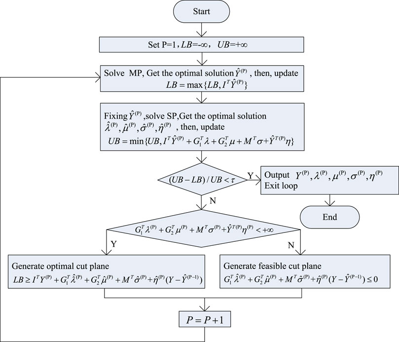
Figure 2. Solution flowchart.

Step 1. Set the loop parameter p = 1 and the initial value of the parameters.

Step 2. Solve the MP and get the optimal solution of binary variables ${\widehat{Y}}^{\left(\mathrm{P}\right)}$. Update the lower bound through $LB=\max \left\{LB,I^T{\widehat{Y}}^{\left(P\right)}\right\}$.

Step 3. Solve the robust dual SP by fixing the condition $Y={\widehat{Y}}^{\left(\mathrm{P}\right)}$ and obtaining the optimal solution ${\widehat{\lambda }}^{\left(\mathrm{P}\right)},{\widehat{\mu }}^{\left(\mathrm{P}\right)},{\widehat{\sigma }}^{\left(\mathrm{P}\right)},{\widehat{\eta }}^{\left(\mathrm{P}\right)}$. Then, update $UB=\min \left\{UB,I^T{\widehat{Y}}^{\left(\mathrm{P}\right)}+G_1^T\lambda +G_2^T\mu +M^T\sigma +{\widehat{Y}}^{T\left(\mathrm{P}\right)}\eta \right\}$, and $UB$ is the upper bound of the solution.

Step 4. Check $\left(UB-LB\right)/UB\le \tau$. If satisfied, output $Y^{\left(\mathrm{P}\right)},{\lambda }^{\left(\mathrm{P}\right)},{\mu }^{\left(\mathrm{P}\right)},{\sigma }^{\left(\mathrm{P}\right)},{\eta }^{\left(\mathrm{P}\right)}$ and exit the loop. Otherwise, go to Step 5.

Step 5. Check the optimal solution of the dual SP; in other words, $G_1^T{\lambda }^{\left(\mathrm{P}\right)}+G_2^T{\mu }^{\left(\mathrm{P}\right)}+M^T{\sigma }^{\left(\mathrm{P}\right)}+{\widehat{Y}}^{T\left(\mathrm{P}\right)}{\eta }^{\left(\mathrm{P}\right)}<+\infty$. If satisfied, go to Step 6. Otherwise, go to Step 7.

Step 6. Generate the optimal cut plane $LB\ge I^T{Y}^{\left(\mathrm{P}\right)}+G_1^T{\widehat{\lambda }}^{\left(\mathrm{P}\right)}+G_2^T{\widehat{\mu }}^{\left(\mathrm{P}\right)}+M^T{\widehat{\sigma }}^{\left(\mathrm{P}\right)}+{\widehat{\eta }}^{\left(\mathrm{P}\right)}\left(Y-{\widehat{Y}}^{\left(\mathrm{P}-1\right)}\right)$ and P = P + 1, and then, go to Step 2.

Step 7. Generate the feasible cut plane $G_1^T{\widehat{\lambda }}^{\left(\mathrm{P}\right)}+G_2^T{\widehat{\mu }}^{\left(\mathrm{P}\right)}+M^T{\widehat{\sigma }}^{\left(\mathrm{P}\right)}+{\widehat{\eta }}^{\left(\mathrm{P}\right)}\left(Y-{\widehat{Y}}^{\left(\mathrm{P}-1\right)}\right)\le 0$ and P = P + 1, and then, go to Step 2.

5 Case study

5.1 Description of the test system

The modified IEEE 24-node system (Probability Methods Subcommittee, 1979) includes 38 existing lines, 9 traditional generator units, 6 wind farms, and 3 photovoltaic power stations, as seen in Figure 3. Compared to the standard IEEE 24-bus system, its grid structure is the same. The difference is that we added photovoltaic and wind farms, with their specific location shown in Figure 3. To reveal how the deep internal influence acts on power grids with different trustworthiness of DR, we set it to vary from 0.0 to 1.0. The value 0.0 means no trust, and 1.0 represents full trust. In other words, as the value increases, the level of trust increases. The time series (e.g., wind, photovoltaic power output, and electricity loads) were extracted from the practical cases obtained in Li H. et al. (2020). In addition, the penetration level of RESs is assumed to be 60% of their installed capacity. The decreased rate of ESS maintenance costs $\hslash$ is set to 5%. To make a trade-off between computational efficiency and accuracy, the k-medoids clustering technique (Park and Jun, 2009) is used instead of solving 8,760 h for the whole year. Each representative period is considered as one scenario, and the scenario probability is obtained from the clustering process. It should be noted that besides several special days, natural days during 1 year can be mainly clustered into working days splicing weekends. Therefore, it is more conducive to the system solution based on the week consisting of two consecutive days. Moreover, ensuring the consideration of the data’s sequential nature and making the benefits of ESSs more obvious, we showed the state for 48 consecutive periods. During these 48 consecutive periods, there is a difference in renewable energy and load.

Figure 3

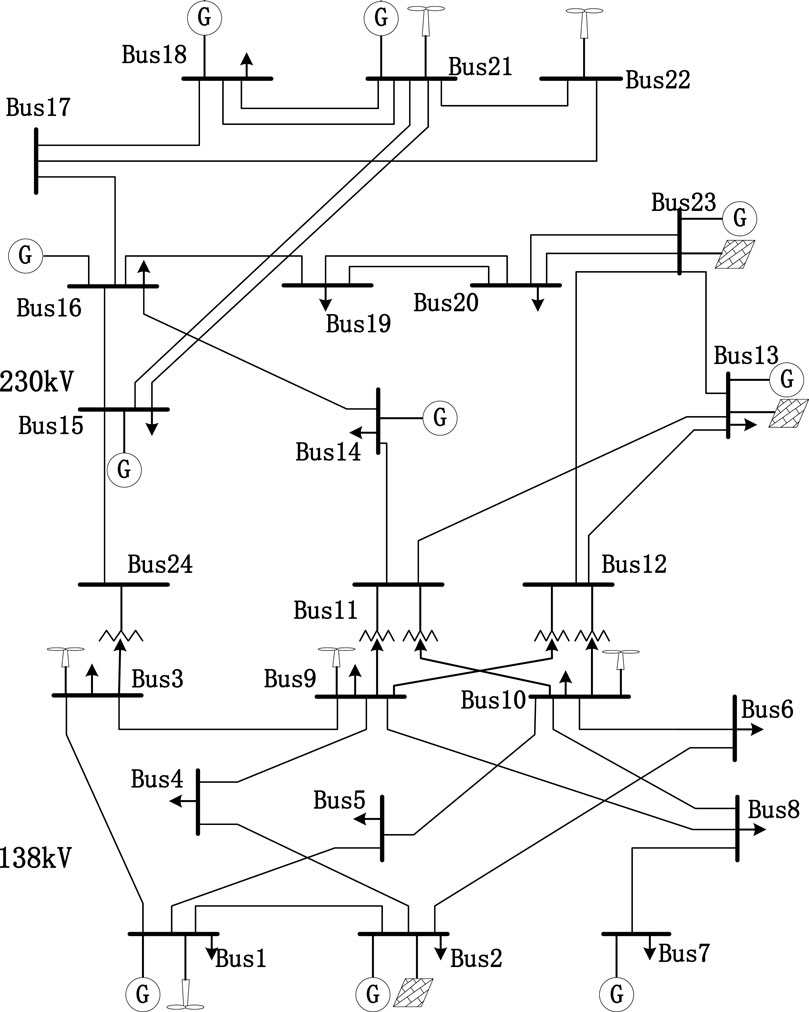
Figure 3. Modified IEEE 24-node system.

On the other hand, the economic data, namely, investment cost, operation cost (i.e., fuel costs, O&M costs, renewable energy spillage costs, and loss load costs, ), and environmental parameters (i.e., CO₂ emission costs), are presented in Table 2. Note that linear generation-cost functions were used for traditional generation units due to their acceptable accuracy and the already complex nature of the optimization problem.

Table 2

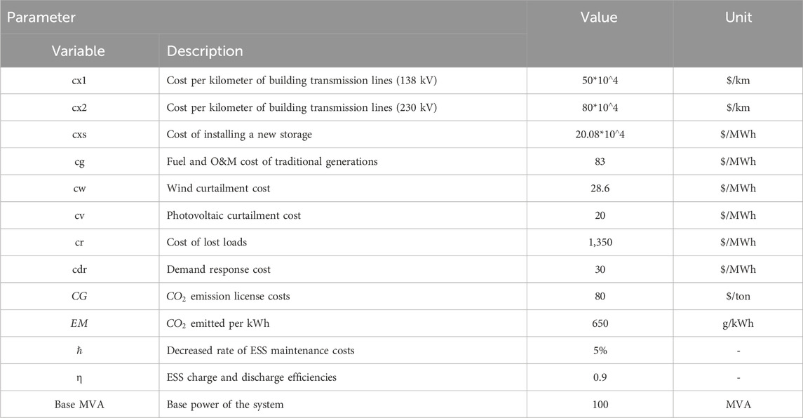
Table 2. Values of several parameters used in the optimization problem.

The simulations have been solved by using Gurobi9.1.1 as the solver. We considered a convergence tolerance of 0.01%. All studies were operated on an Intel-Core i7 (64-bit) 3.4-GHz individual laptop with 16GB RAM.

5.2 Simulation results and discussions

To understand what the impact of varied resources and technologies on power system planning is, three different experiments were conducted: 1) case 1 ignores the trustworthiness of DR, that is, all available DR responses, only considering the difference of one single ESS capacity, in which whether to install and where to construct are both considered. In this case, we find a suitable size for one single ESS capacity because it affects the maintenance costs in this system. 2) It is fixed according to the suitable size of each single ESS. Case 2 only considers the impact of different trustworthiness of DR. It should be noted that in this case, the objective function does not contain Equations 9, 10. 3) Based on case 2, besides minimizing total costs, CO₂ emissions are considered simultaneously, and a trade-off is made between them. Here, cost-savings and reducing CO₂ emissions are of equal importance.

5.2.1 Ignoring the trustworthiness of DR

In this experiment, to select an appropriate size of ESSs, we only consider single-size changes, which includes all available DR responses. Table 3 demonstrates the expansion planning results of this optimization model. The location, degradation of ESSs, and whole-system CO₂ emission costs were included. In addition, the decreased amount of ESS maintenance costs has been contained in operation costs. It is clear that with different sizes of each ESS, their optimal location changes. The new energy storage stations need to be installed more when their single size is small because the investment cost is proportional to its capacity, and the system needs more storage to improve its flexibility.

Table 3

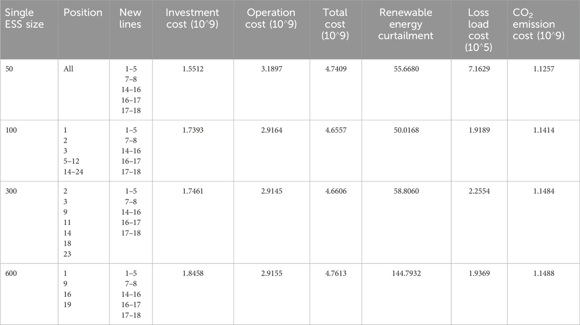
Table 3. Simulation results of the power system with different ESS sizes.

Specifically, first of all, we compared the first two rows. Although the single capacity of the first row is small and its investment cost is low, however, its operation cost is higher. This is partly due to the surge of renewable energy curtailment, loss of load, and ESS maintenance costs. Moreover, the high flexibility requirements of some nodes are not fully met. Afterward, the last three lines are compared. As the individual ESS capacity increases, the investment cost increases, but the operation cost changes slightly. This is because renewable energy curtailment and loss of load increases, while ESS maintenance costs decrease. In other words, the number of ESSs is lessened so that the labor cost is reduced, which is related to the maintenance cost. Overall, the total cost increases as the individual ESS capacity increases. In other words, the capacity of ESSs has a close impact on power system expansion planning.

What needs to be illustrated is that when the single ESS capacity is larger, CO₂ emission costs change very slightly. This is because the penetration of renewable energy is not very high. So when the individual size is larger, the number that should be newly installed will be reduced. It is worth mentioning that the degradation of ESSs was taken into account, so the storage investment cost was more grounded in reality. In addition, renewable energy curtailment and loss load were the lowest when the single storage capacity was 100 MWh. Finally, taking renewable energy curtailment, loss of load, and total costs into account, individual ESS capacity will be appropriate at 100 MWh in this system.

Figure 4 shows the details of charge–discharge energy and the SOC of a newly installed ESS connected to bus 9 in a representative period. The initial value of ESSs is 0.14 p.u., and it needs to stay the same at the beginning and at the end of one period. As can be seen, the charging time always appears at low load hours and vice versa on the contrary. Because the RES output changed significantly in two consecutive periods, the charging and discharging behavior changed as well. Note that the experiments we performed in this section with available DR are fixed at 0.02, and their trustworthiness is 1.0.

Figure 4

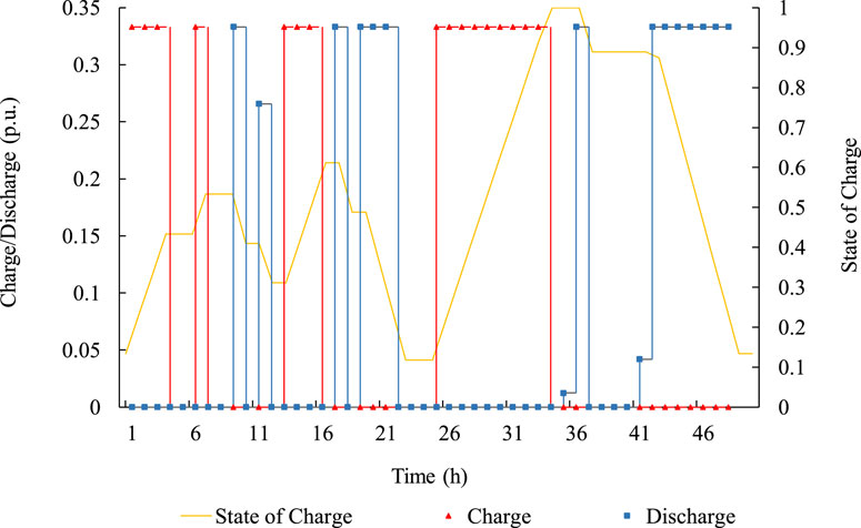
Figure 4. Details of a newly installed ESS in one representative period.

Figure 5 shows the operating points of the source and demand status under the condition that the ESS capacity is 100 MWh and its actual DR is set at 0.02 in one representative period. As can be seen, at the beginning of 1–6 h, its load is relatively small, and charging occurs (see the yellow bar below the x-axis). When time goes to 8–11, due to load increases, the system preferentially discharges from ESSs to meet the demand (see the blue bars in this figure). In 13–16 h, the whole output of renewable energy surges. On one hand, the output of traditional generations is reduced because of their high operating costs and emissions costs. On the other hand, the power system charges ESSs in preparation for evening peak load hours (also see the yellow bar below the x-axis). Then, the system enters the night charging period. The next day is much the same, except for the decrease in photovoltaic power output, and there is a slight loss of load in 41–45. This is in line with the discussion presented above.

Figure 5

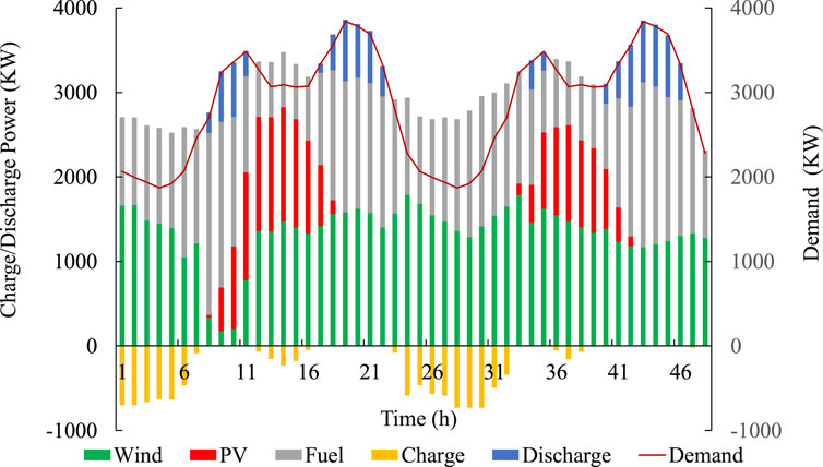
Figure 5. Sources and demand status in one representative period.

5.2.2 Different trustworthiness of DR

To compare what impacts act on the expansion planning optimization problem with different trustworthiness of DR, we performed the following experiments. In this section, the individual ESS capacity is set at 100 MWh, as discussed before. Simulation results are shown in Table 4. It should be noted that the second row in Table 4 should be the same as in Table 3. This is because the available DR is fixed at 0.2 with its trustworthiness setting at 0.1, which equals the actual DR being set at 0.02. As shown in each column, the expanded transmission line changes slightly with different trustworthiness of DR. However, the number of newly installed ESSs decreases when the trustworthiness of DR increases. It also causes little change in CO₂ emission costs when the actual DR increases. This is because DR plays the role of peak cutting and valley filling, and the total load remains constant.

Table 4

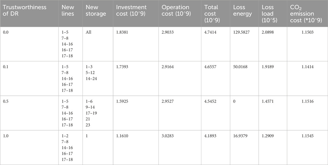
Table 4. Simulation results of the system with different DR without considering the impact of CO₂ emissions.

The investment cost narrows down due to new ESSs that need to be installed being reduced when the trustworthiness of DR increases. So, even though the unavoidable DR subsidy cost grows, the value of both loss energy and loss load decreases, which leads to the operation cost increasing slightly. Thus, in a word, the total cost of this expansion-planning problem is reduced because of the higher trustworthiness of DR. In other words, the appropriate application of DR can help reduce expansion costs and lessen loss load and RES curtailment. Note that the experiments we performed in this section with available DR are fixed at 0.2.

Figure 6 shows the participation situation of different trustworthiness of the available DR at bus18. In general, the higher the trustworthiness of DR, the more actual DR participates in the system. As can be seen, the positive value of participating DR equals the negative one in 48 h. Moreover, when the electricity demand is high, DR is mostly positive. While the electricity demand is low, and vice on the contrary. However, the symbol of DR is not always positive in peak load hours due to its abundant flexibility resources and renewable energy volatility. See hours 13, 14, 15, and 16. Therefore, DR can improve the flexibility of the system. In hours 18 and 21, the actual participating DR is not at its maximum. This illustrates the need for precise control of DR rather than crude subsidies.

Figure 6

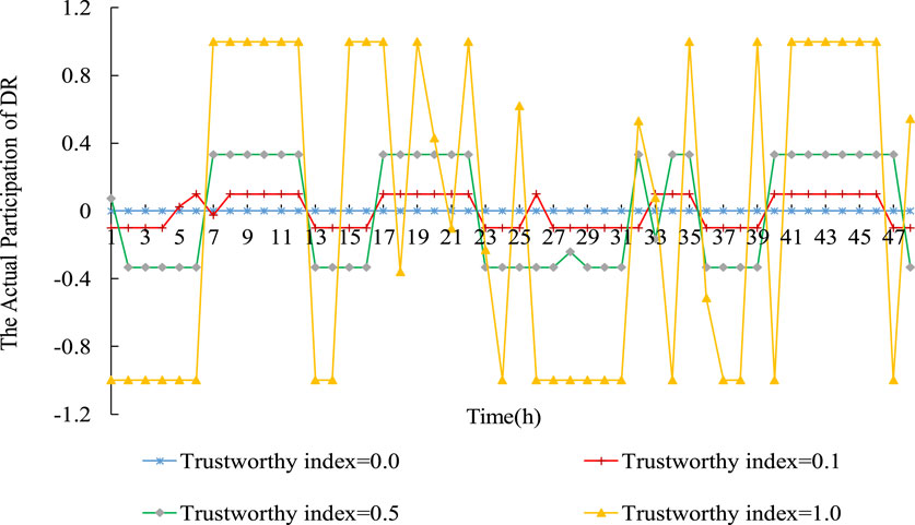
Figure 6. Different trustworthiness of DR at bus18.

5.2.3 A trade-off between minimizing total costs and reducing CO₂ emissions

Since GHG emissions have a heavy influence on our environment, obtaining a sustainable and environmentally friendly power system became the global common goal. It is not appropriate to aim only at cost minimization because new technology is generally expensive at the beginning stage but are environmentally friendly. Therefore, this study makes a trade-off between minimizing total costs and reducing CO₂ emissions. We assume these two goals are of equal importance in this paper. In other words, Equations 9, 10 are included in the objective function. As shown in each column of Table 5, the number of newly installed ESSs also decreases as the trustworthiness of DR increases. However, the newly installed number should be more compared with that of the previous experiment (case 2), which only focuses on cost minimization (shown in Table 4). The most important factor is that CO₂ emission costs decreased with each different trustworthiness of DR, as compared to the cost minimization experiment. Specifically, the data on CO₂ emission cost reduced from 1.1545$ to 1.1312$, which reduced by 2.1%, when the trustworthiness of DR was 1.0.

Table 5

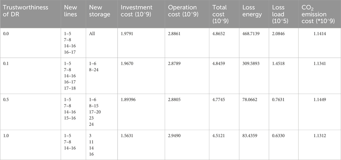
Table 5. Simulation results with different trustworthiness of DR considering the impact of CO₂ emissions.

Figure 7 presents an intuitive comparison of case 2 (only considering cost minimization) and case 3 (a trade-off between minimizing total costs and reducing CO₂ emissions). On equal terms compared to the previous case, although fewer new lines need to be constructed to strengthen the transmission network, however, more ESSs need to be installed. Thus, the investment cost increased considerably as it went up from 1.7393*10^9$ (the second row and fourth column in Table 4) to 1.9670*10^9$ (the second row and fourth column in Table 5). Moreover, the operation cost decreased slightly in case 3, with its value decreasing from 2.9164*10^9$ to 2.8789*10^9$. Thus, in a word, the total cost is larger than the condition without considering CO₂ emissions. Specifically, statistics of total cost rose from 4.6557*10^9$ to 4.8459*10^9$, an increase of 3.9%, when the trustworthiness of DR was 0.1. To maximize renewable energy consumption, the system takes priority utilization of all newly installed ESSs rather than conventional generations. In case 3, the loss load costs were reduced for each different trustworthiness of the DR condition. It indicated that the power supply reliability was improved.

Figure 7

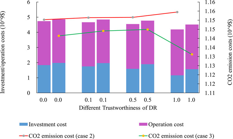
Figure 7. Comparison of considering only cost minimization and considering both minimizing costs and reducing CO₂ emissions.

To sum up, case 3 is a more appropriate strategy for the following reasons: 1) it can help reduce GHG emissions, which is consistent with the current environmental protection concept; 2) it improves power system reliability because it uses flexible resources preferentially and lessens the value of loss load; 3) it defers transmission expansion due to abundant flexible resources. Thus, it alleviated the bottleneck of unbalanced development of the short-term renewable energy expansion period and the long-term transmission expansion period.

5.2.4 Analysis of the effectiveness of the dual-decomposition method

To verify the effectiveness of the dual-decomposition algorithm, we compared the simulation results of case 3, where the trustworthiness of DR is set to 1.0, using both the centralized algorithm and the dual-decomposition algorithm. As shown in Table 6, it can be observed that regardless of the solving algorithm, the newly constructed lines and ESSs are identical, resulting in the same investment cost for both algorithms. Moreover, the two algorithms yield the same cost for GHG emissions. Additionally, the centralized algorithm produces slightly different RES curtailment and loss-load costs compared to the decomposition algorithm. This leads to a small difference in total costs. This discrepancy is due to the convergence tolerance being set at 0.01% during program design, but it does not affect the final results.

Table 6

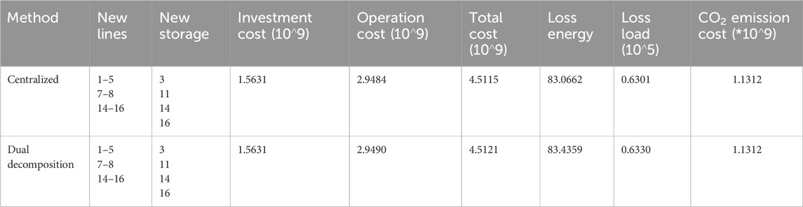
Table 6. Simulation results using different solving methods when the trustworthiness of DR is 1.0

6 Conclusion

This paper proposed a robust coordinated planning model for power systems, in which large shares of variable renewable energy are integrated. For the sake of accuracy and efficiency, piecewise linearization, big-M method, and dual decomposition were introduced due to the already complex nature of the optimization problem. The inevitable uncertainty (variable RESs and demand) is described by polyhedral sets. To understand the impact of varied resources and technologies (such as wind power, photovoltaic resources, ESSs, and the trustworthiness of DR) on the development of power system planning, several computational experiments are presented. First, the capacity, location, and degradation of ESSs have a close impact on power system expansion planning. It is necessary to select an appropriate capacity and location for every single energy storage station in the planning stage. Second, higher trustworthiness of DR can help reduce the total expansion costs. However, it has little impact on GHG emissions if we consider cost minimization only. The last study makes a trade-off between minimizing total costs and reducing CO₂ emissions. According to this, a more sustainable and environmentally friendly power system was obtained. Moreover, it improves power system reliability and alleviates the unbalanced development of the short-term renewable energy expansion period and the long-term transmission expansion period.

Data availability statement

The raw data supporting the conclusions of this article will be made available by the authors, without undue reservation.

Author contributions

PF: data curation, software, validation, writing–original draft, and writing–review and editing. CC: methodology, supervision, and writing–review and editing. LW: supervision, visualization, and writing–review and editing.

Funding

The author(s) declare that financial support was received for the research, authorship, and/or publication of this article. This work was supported by the Yancheng Fundamental Research Program. Paper no. YCBK2023010.

Conflict of interest

The authors declare that the research was conducted in the absence of any commercial or financial relationships that could be construed as a potential conflict of interest.

Publisher’s note

All claims expressed in this article are solely those of the authors and do not necessarily represent those of their affiliated organizations, or those of the publisher, the editors, and the reviewers. Any product that may be evaluated in this article, or claim that may be made by its manufacturer, is not guaranteed or endorsed by the publisher.

Supplementary material

The Supplementary Material for this article can be found online at: https://www.frontiersin.org/articles/10.3389/fenrg.2024.1384760/full#supplementary-material

References

Aghajani, G. R., Shayanfar, H. A., and Shayeghi, H. (2017). Demand side management in a smart micro-grid in the presence of renewable generation and demand response. Energy 126, 622–637. doi:10.1016/j.energy.2017.03.051

CrossRef Full Text | Google Scholar

Alahmad, A. K. (2023). Voltage regulation and power loss mitigation by optimal allocation of energy storage systems in distribution systems considering wind power uncertainty. J. Energy Storage 59, 106467. doi:10.1016/j.est.2022.106467

CrossRef Full Text | Google Scholar

Al-Shetwi, A. Q. (2022). Sustainable development of renewable energy integrated power sector: trends, environmental impacts, and recent challenges. Sci. Total Environ. 822, 153645. doi:10.1016/j.scitotenv.2022.153645

PubMed Abstract | CrossRef Full Text | Google Scholar

Cheng, Y., Zhang, N., Lu, Z., and Kang, C. (2019). Planning multiple energy systems toward low-carbon society: a decentralized approach. IEEE Trans. Smart Grid 10 (5), 4859–4869. doi:10.1109/TSG.2018.2870323

CrossRef Full Text | Google Scholar

Dehghan, S., Amjady, N., and Aristidou, P. (2020). A robust coordinated expansion planning model for wind farm-integrated power systems with flexibility sources using affine policies. IEEE Syst. J. 14 (3), 4110–4118. doi:10.1109/JSYST.2019.2957045

CrossRef Full Text | Google Scholar

Dehghan, S., Amjady, N., and Conejo, A. J. (2017). Adaptive robust transmission expansion planning using linear decision rules. IEEE Trans. Power Syst. 32 (5), 4024–4034. doi:10.1109/TPWRS.2017.2652618

CrossRef Full Text | Google Scholar

European Commission, Energy Roadmap 2050 (2011). Brussels, Belgium, EU COM (2011) 885 final, 2011. Available at: http://ec.europa.eu/energy/energy2020/roadmap/index_en.htm.

Google Scholar

Hamzehkolaei, F. T., Amjady, N., and Bagheri, B. (2021). A two-stage adaptive robust model for residential micro-CHP expansion planning. J. Mod. Power Syst. Clean Energy 9 (4), 826–836. doi:10.35833/MPCE.2021.000001

CrossRef Full Text | Google Scholar

Hu, J., Wang, Y., and Dong, L. (2024). Low carbon-oriented planning of shared energy storage station for multiple integrated energy systems considering energy-carbon flow and carbon emission reduction. Energy 290, 130139. doi:10.1016/j.energy.2023.130139

CrossRef Full Text | Google Scholar

Jafari, M., Botterud, A., and Sakti, A. (2022). Decarbonizing power systems: a critical review of the role of energy storage. Energy Rev. 158, 112077. doi:10.1016/j.rser.2022.112077

CrossRef Full Text | Google Scholar

Jiang, X., Jin, Y., Zheng, X., Hu, G., and Zeng, Q. (2020). Optimal configuration of grid-side battery energy storage system under power marketization. Appl. Energy 272, 115242. doi:10.1016/j.apenergy.2020.115242

CrossRef Full Text | Google Scholar

Jiang, Y., Ren, Z., and Li, W. (2024). Committed carbon emission operation region for integrated energy systems: concepts and analyses. IEEE Trans. Sustain. Energy 15 (2), 1194–1209. doi:10.1109/TSTE.2023.3330857

CrossRef Full Text | Google Scholar

Li, H., Lu, Z., Qiao, Y., and Zhang, B. (2020b). Flexibility test system. Available at: https://github.com/HaoLi9401/DatasetofflexibilitytestsystemFTS-213.

Google Scholar

Li, J., Li, Z., Liu, F., Ye, H., Zhang, X., Mei, S., et al. (2018). Robust coordinated transmission and generation expansion planning considering ramping requirements and construction periods. IEEE Trans. Power Syst. 3 (1), 268–280. doi:10.1109/TPWRS.2017.2687318

CrossRef Full Text | Google Scholar

Li, J., Lu, B., Wang, Z., and Zhu, M. (2021b). Bi-level optimal planning model for energy storage systems in a virtual power plant. Renew. Energy 165, 77–95. doi:10.1016/j.renene.2020.11.082

CrossRef Full Text | Google Scholar

Li, J., Yang, B., Huang, J., Guo, Z., Wang, J., Zhang, R., et al. (2023). Optimal planning of electricity–hydrogen hybrid energy storage system considering demand response in active distribution network. Energy 273, 127142. doi:10.1016/j.energy.2023.127142

CrossRef Full Text | Google Scholar

Li, Z., Wu, L., Xu, Y., and Zheng, X. (2021a). Stochastic-weighted robust optimization based bilayer operation of a multi-energy building microgrid considering practical thermal loads and battery degradation. IEEE Trans. Sustain. Energy 13 (2), 668–682. doi:10.1109/TSTE.2021.3126776

CrossRef Full Text | Google Scholar

Li, Z., Xu, Y., Feng, X., and Wu, Q. (2020a). Optimal stochastic deployment of heterogeneous energy storage in a residential multienergy microgrid with demand-side management. IEEE Trans. Industrial Inf. 17 (2), 991–1004. doi:10.1109/TII.2020.2971227

CrossRef Full Text | Google Scholar

Liu, J., Cheng, H., Zeng, P., and Yao, L. (2018). Rapid assessment of maximum distributed generation output based on security distance for interconnected distribution networks. Int. J. Electr. Power Energy Syst. 101, 13–24. doi:10.1016/j.ijepes.2018.03.018

CrossRef Full Text | Google Scholar

Liu, J., Tang, Z., Zeng, P. P., Li, Y., and Wu, Q. (2022). Distributed adaptive expansion approach for transmission and distribution networks incorporating source-contingency-load uncertainties. Int. J. Electr. Power Energy Syst. 136, 107711. doi:10.1016/j.ijepes.2021.107711

CrossRef Full Text | Google Scholar

Mansouri, S. A., Ahmarinejad, A., Sheidaei, F., Javadi, M. S., Jordehi, A. R., Nezhad, A. E., et al. (2022). A multi-stage joint planning and operation model for energy hubs considering integrated demand response programs. Int. J. Electr. Power Energy Syst. 140, 108103. doi:10.1016/j.ijepes.2022.108103

CrossRef Full Text | Google Scholar

Olsen, D. J., Dvorkin, Y., Fernandez-Blanco, R., and Ortega-Vazquez, M. A. (2018). Optimal carbon taxes for emissions targets in the electricity sector. IEEE Trans. Power Syst. 33 (6), 5892–5901. doi:10.1109/TPWRS.2018.2827333

CrossRef Full Text | Google Scholar

Paris agreement (2015). United nations framework convention on climate change, UN. Available at: https://unfccc.int/sites/default/files/english_paris_agreement.pdf.

Google Scholar

Park, H.-S., and Jun, C.-H. (2009). A simple and fast algorithm for K-Medoids clustering. Expert Syst. Appl. 36 (2), 3336–3341. doi:10.1016/j.eswa.2008.01.039

CrossRef Full Text | Google Scholar

Pirouzi, S., and Aghaei, J. (2019). Mathematical modeling of electric vehicles contributions in voltage security of smart distribution networks. Simul. Trans. Soc. Model. Simul. Int. 95 (5), 429–439. doi:10.1177/0037549718778766

CrossRef Full Text | Google Scholar

Pirouzi, S., Aghaei, J., Latify, M. A., Yousefi, G. R., and Mokryani, G. (2018). A robust optimization approach for active and reactive power management in smart distribution networks using electric vehicles. IEEE Syst. J. 12 (3), 2699–2710. doi:10.1109/JSYST.2017.2716980

CrossRef Full Text | Google Scholar

Pirouzi, S., Aghaei, J., Niknam, T., Shafie-Khah, M., Vahidinasab, V., and Catalao, J. P. S. (2017). Two alternative robust optimization models for flexible power management of electric vehicles in distribution networks. Energy 141, 635–651. doi:10.1016/j.energy.2017.09.109

CrossRef Full Text | Google Scholar

Probability Methods Subcommittee (1979). IEEE reliability test system. IEEE Trans. Power App. Syst. 98 (6), 2047–2054. doi:10.1109/TPAS.1979.319398

CrossRef Full Text | Google Scholar

Qi, H. J., Yue, H., Zhang, J. F., and Lo, K. L. (2021). Optimisation of a smart energy hub with integration of combined heat and power, demand side response and energy storage. Energy 234, 121268. doi:10.1016/j.energy.2021.121268

CrossRef Full Text | Google Scholar

Ramos-Real, F. J., Barrera-Santana, J., Ramírez-Díaz, A., and Perez, Y. (2018). Interconnecting isolated electrical systems. The case of Canary Islands. Energy Strategy Rev. 22, 37–46. doi:10.1016/j.esr.2018.08.004

CrossRef Full Text | Google Scholar

Shi, Z., Wang, W., Huang, Y., Li, P., and Dong, L. (2022). Simultaneous optimization of renewable energy and energy storage capacity with the hierarchical control. CSEE J. Power Energy Syst. 8 (1), 95–104. doi:10.17775/CSEEJPES.2019.01470

CrossRef Full Text | Google Scholar

Summary for policymakers (2021). In: climate Change 2021: the physical science basis. contribution of working group I to the sixth assessment report of the inter-governmental panel on climate change. IPCC, 3–32. doi:10.1017/9781009157896.001

CrossRef Full Text | Google Scholar

Tan, H., Ren, Z., Yan, W., Wang, Q., and Mohamed, M. A. (2021). A wind power accommodation capability assessment method for multi-energy microgrids. IEEE Trans. Sustain. Energy 12 (4), 2482–2492. doi:10.1109/TSTE.2021.3103910

CrossRef Full Text | Google Scholar

Velloso, A., Street, A., Pozo, D., Arroyo, J. M., and Cobos, N. G. (2020). Two-stage robust unit commitment for co-optimized electricity markets: an adaptive data-driven approach for scenario-based uncertainty sets. IEEE Trans. Sustain. Energy 11 (2), 958–969. doi:10.1109/TSTE.2019.2915049

CrossRef Full Text | Google Scholar

Velloso, A., and Van Hentenryck, P. (2021). Combining deep learning and optimization for preventive security-constrained DC optimal power flow. IEEE Trans. Power App. Syst. 36 (4), 3618–3628. doi:10.1109/TPWRS.2021.3054341

CrossRef Full Text | Google Scholar

Xu, B., Oudalov, A., Ulbig, A., Andersson, G., and Kirschen, D. S. (2018). Modeling of lithium-ion battery degradation for cell life assessment. IEEE Trans. Smart Grid 9 (2), 1131–1140. doi:10.1109/TSG.2016.2578950

CrossRef Full Text | Google Scholar

Zappa, W., Junginger, M., and van den Broek, M. (2019). Is a 100% renewable European power system feasible by 2050? Appl. Energy 233–234, 1027–1050. doi:10.1016/j.apenergy.2018.08.109

PubMed Abstract | CrossRef Full Text | Google Scholar

Zhang, M., Fang, J., Ai, X., Shuai, H., Yao, W., He, H., et al. (2020). Feasibility identification and computational efficiency improvement for two-stage RUC with multiple wind farms. IEEE Trans. Sustain. Energy 11 (3), 1669–1678. doi:10.1109/TSTE.2019.2936581

CrossRef Full Text | Google Scholar

Zheng, X., Qu, K., Lv, J., Li, Z., and Zeng, B. (2021). Addressing the conditional and correlated wind power forecast errors in unit commitment by distributionally robust optimization. IEEE Trans. Sustain. Energy 12 (2), 944–954. doi:10.1109/TSTE.2020.3026370

CrossRef Full Text | Google Scholar

Nomenclature