A two-stage optimization configuration model for multi-type flexible resource considering spatiotemporal response characteristics

As China gradually transitions towards a low-carbon energy structure, the proportion of grid-connected new energy sources like wind and solar power continues to increase. To ensure the safe and reliable operation of the power system while meeting the capacity planning for future new energy installations, there is a need for flexible resources with corresponding adjustment capabilities in the power system. In response to this situation, this paper presents an optimization model for the allocation of multiple types of flexible resources that takes into account spatiotemporal response characteristics. Firstly, a flexibility evaluation model is developed based on spatial and temporal response characteristics. Flexibility evaluation indices, such as flexibility average deficit and flexibility coverage index, are constructed. These indices are used for screening nodes with inadequate flexibility in the power system and analyzing the flexibility adequacy at various nodes. Next, the adjustment characteristics of multiple types of flexible resources are analyzed, and a model for their adjustment capabilities is established. Finally, by considering constraints based on time flexibility evaluation indices, a two-stage optimization model for flexible resource allocation is constructed. This model leverages the multiscale matching characteristics between flexibility resources and the fluctuation patterns of new energy sources to guide the allocation of flexible resources at nodes with insufficient flexibility. The effectiveness and applicability of the proposed flexible resource allocation method are validated using the IEEE 9-node system.

1 Introduction

With the rise of the green and low-carbon concept and the continuous deepening of energy transition, to reduce dependence on traditional fossil fuels and decrease carbon emissions (Huang et al., 2023), and in response to the challenges of climate change, the grid integration ratio of new energy sources such as wind and solar will continue to expand, posing higher demands on the flexibility of the power system due to their randomness and uncertainty (Turk et al., 2020).

Currently, there have been numerous studies on the assessment of flexibility in power systems with a high proportion of renewable energy. Existing evaluation indicators and methods on flexibility can be broadly categorized as deterministic and probabilistic. Yan et al. conducted a practical framework study on the flexibility evaluation of power systems at different time scales, considering the uncertainty of renewable energy through the Monte Carlo method (Yan et al., 2020). Lu et al. proposed a novel assessment method based on the probability distribution of flexibility abundance, capable of linearly reflecting the relationship between flexibility shortage and renewable energy reduction (Lu et al., 2018). Tang et al. proposed flexibility evaluation indicators from three perspectives: intra-area supply-demand balance, intra-area power flow distribution, and inter-area transmission capacity (Tang et al., 2020). Stephen et al. introduced a novel metric using the concept of inter-layer pipe bundling to assess the integrated flexibility of natural gas and electricity (Clegg and Mancarella, 2016). Guo et al. introduced a production simulation method using an improved generalized generating function as a flexibility evaluation tool and proposed a flexibility measurement method based on the definition of flexibility and physical mechanisms (Guo et al., 2020). The aforementioned literature collectively indicates that the application of flexibility evaluation methods and indicators can assist power system planners and operators in gaining a better understanding of system flexibility. It enables them to formulate corresponding strategies to cope with the fluctuations in renewable energy output and load. Simultaneously, the assessment of power system flexibility is a multi-layered, multidimensional issue that requires comprehensive consideration of spatial, temporal, and resource-related factors. The traditional flexibility evaluation only analyzes from a single dimension of time or space, without considering the temporal and spatial coupling characteristics of the system, and the evaluation results deviate from the reality. Therefore, it is necessary to conduct a refined evaluation starting from the spatiotemporal characteristics of flexibility resources, providing new insights for enhancing system flexibility and optimizing resource allocation.

In terms of the optimization of flexibility resource allocation, due to the large variability of flexibility resource regulation characteristics at different scales, it is often necessary to consider how to complement the allocation of different types of flexibility resources to meet the different dimensions of the flexibility needs of the new power system. Zhang et al. proposed a multi-flexibility resource collaborative configuration optimization model, considering the Stackelberg game relationship between the flexibility adjustment demands and capabilities of different segments of the power system under various fluctuation scenarios (Ting and Yunna, 2024). Ren et al. comprehensively considered the economic, security, and flexibility aspects of the system, establishing a dual-layer operational planning joint optimization model for flexibility resources (Ren et al., 2020). Ji et al. developed a mixed-integer linear programming model to optimize the design and scheduling of hybrid energy systems, utilizing rooftop photovoltaics and solid waste biomass to meet electricity demands (Ji et al., 2022). Li et al. proposed a new perspective on modeling and planning the flexibility resources at multiple time scales in power systems with high penetration of variable renewable energy. This approach transforms the operational boundaries of flexibility resources into characteristic domains (Li et al., 2022). Zhang et al. proposed a two-dimensional mixed energy storage optimization configuration model for a novel power system with the coupling of multiple flexible resources, aiming to meet the diverse flexibility adjustment requirements at various stages of the novel power system (Zhang et al., 2023). The models in the aforementioned literature often comprehensively consider the coupling of planning and operational aspects, leading to a complex computational process. Existing literature typically plans operations on a single time scale and does not consider grid flexibility at finer time scales. At the same time, existing studies have not fully explored how to optimize power system configuration while simultaneously considering the economic and flexibility resource characteristics. This optimization aims to maximize the potential of flexible resources such as solar-thermal power stations and energy storage.

In response to the aforementioned limitations, this paper proposes a multi-type flexibility resource configuration optimization model that takes into account spatiotemporal response characteristics. Firstly, starting from the net load demand and resource allocation status quo of each node, the flexibility evaluation model based on spatial response characteristics screens the flexibility-deficient nodes and determines the specific location of the allocated flexibility resources. Secondly, considering the multi-timescale fluctuation characteristics of renewable energy/load, the flexibility evaluation constraints based on the time response characteristics, and with the objective of minimizing the investment and construction cost and operation cost of flexibility resources, the optimization model for the allocation of multiple types of flexibility resources is established. Finally, the effectiveness of the configuration optimization model proposed in this paper is verified by IEEE 9-node system simulation.

2 Spatiotemporal flexibility evaluation model for power systems

2.1 Flexibility evaluation model based on spatial response characteristics

To determine the optimal spatial locations for the configuration of flexible resources, it is necessary to construct a flexibility assessment model based on spatial response characteristics, considering the net load demands and resource allocation status at each node. Firstly, setting the evaluation time scale to 1 h, the power system network structure, resource allocation status, and predicted values of node net load are obtained. With the objective of minimizing the total flexibility deficit in the system, an optimization model for unit combination based on spatial response characteristics is formulated, resulting in the baseline output scheme. The objective function is shown in Formula (1).

$minf={\displaystyle \sum _{t=1}^{T_1}}{\displaystyle \sum _m^{N_m}}\left|P_{lack,t}^m\right|(1)$

Where, $P_{lack,t}^m$ represents the flexibility deficit at node $m$ at time $t$, with a positive value indicating insufficient downward ramping capability and a negative value indicating insufficient upward ramping capability.

Next, the average flexibility deficit within the time period is calculated as the evaluation indicator to reflect the flexibility deficiency at each node. This provides a reference for screening nodes with insufficient flexibility. The function is shown in Formula (2).

$P_{lack}^m=\frac{1}{T_1}{\displaystyle \sum _{t=1}^{T_1}}\left|P_{lack,t}^m\right|(2)$

Where, $P_{lack}^m$ represents the average flexibility deficit at node $m$.

The constraint conditions are as follows:

1) This paper assume that network losses are ignored and only power balance is considered. The unit output scheduling at each node in the region must meet the predicted net load demand. The function is shown in Formula (3).

${\displaystyle \sum _{k=1}^{N_k}}{P}_{k,t}^m+{\displaystyle \sum _{n\in N_m}}{P}_{mn,t}=P_{net,t}^m+P_{lack,t}^m+P_{ex,t}^m(3)$

Where, $P_{k,t}^m$ represents the planned output of unit $k$ at node $m$ at time $t$, the unit types include all power generation resources and flexibility resources within the system; $P_{net,t}^m$ represents the net load forecast value for node $m$ at time $t$. $P_{mn,t}$ represents the power interaction between nodes $m$ and $n$ at time $t$. $P_{lack,t}^m$ is the difference between the load forecast and the wind power forecast; $P_{ex,t}^m$ is the outgoing power demand of node $m$ at time $t$.

2) To prevent all units’ reserve output from concentrating on meeting the flexibility requirements of a specific node, the flexibility deficit at each node must satisfy an upper limit constraint. The function is shown in Formula (4).

$\left\{\begin{array}{c}-P_{lack,t}^m\le P_{lack,\mathit{max}}^{up},P_{lack,t}^m\le 0\\ P_{lack,t}^m\le P_{lack,\mathit{max}}^{dn},P_{lack,t}^m>0\end{array}\right.(4)$

Where, $P_{lack,\mathit{max}}^{up}$ and $P_{lack,\mathit{max}}^{dn}$ are the upper limit values of the upward and downward flexibility deficits at each node.

3) The reserve output provided by each unit must satisfy an upper limit constraint. The function is shown in Formula (5).

$\left\{\begin{array}{c}0\le R_{k,t}^{m,up}\le ∆P_{k,m}\\ 0\le R_{k,t}^{m,dn}\le ∆P_{k,m}\end{array}\right.(5)$

Where, $R_{k,t}^{m,up}$ and $R_{k,t}^{m,dn}$ represent the upward and downward reserve output that unit $k$ under node $m$ can provide at time t; $∆P_{k,m}$ denotes the ramping rate of unit k under nod $m$.

4) The output of each unit needs to satisfy the constraints of output upper and lower limits and ramping constraints. The function is shown in Formula (6).

$\left\{\begin{array}{l}{s}_k^m{P}_{k,\mathit{min}}^m\le P_{k,t}^m+R_{k,t}^{m,up}\le s_k^m{P}_{k,\mathit{max}}^m\\ s_k^m{P}_{k,\mathit{min}}^m\le P_{k,t}^m-R_{k,t}^{m,dn}\le s_k^m{P}_{k,\mathit{max}}^m\\ -∆P_k^m\le \left(P_{k,t}^m+R_{k,t}^{m,up}\right)-\left(P_{k,t-1}^m-R_{k,t-1}^{m,dn}\right)\le ∆P_k^m\end{array}\right.(6)$

Where, $P_{k,\mathit{max}}^m$ and $P_{k,\mathit{min}}^m$ represent the upper and lower limits of the output of unit $k$ under node $m$; $s_k^m$ represents the operating state of unit $k$ under node $m$.

5) Power interaction between nodes is subject to network constraints. The function is shown in Formula (7).

$\left\{\begin{array}{c}-P_{mn,\mathit{max}}<P_{mn,t}+R_{mn,t}^{up}<P_{mn,\mathit{max}}\\ -P_{mn,\mathit{max}}<P_{mn,t}+R_{mn,t}^{down}<P_{mn,\mathit{max}}\end{array}\right.(7)$

Where, $P_{mn,\mathit{max}}$ represents the upper limit of power interaction between node $m$ and node $n$; $R_{mn,t}^{up}$ and $R_{mn,t}^{down}$ represent the upward and downward reserves that nodes $m$ and $n$ can interact with at time $t$.

6) Each node needs to satisfy the spinning reserve constraint at a 1-h time scale. The function is shown in Formula (8).

$\left\{\begin{array}{c}{R}_{up,t}^m={\displaystyle \sum _{k=1}^{N_k}}{R}_{k,t}^{m,up}+{\displaystyle \sum _{n\in N_m}}{R}_{mn,t}^{up}\ge {\alpha }_{wpp}^{up}{P}_{wpp,t}^m+{\alpha }_{pv}^{up}{P}_{pv,t}^m+{\alpha }_{load}^{up}{P}_{load,t}^m\\ R_{dn,t}^m={\displaystyle \sum _{k=1}^{N_k}}{R}_{k,t}^{m,dn}+{\displaystyle \sum _{n\in N_m}}{R}_{mn,t}^{dn}\ge {\alpha }_{wpp}^{dn}{P}_{wpp,t}^m+{\alpha }_{pv}^{dn}{P}_{pv,t}^m+{\alpha }_{load}^{dn}{P}_{load,t}^m\end{array}\right.(8)$

Where, $R_{up,t}^m$ and $R_{dn,t}^m$ are the total upward/downward spinning reserve output of node $m$ at time $t$; ${\alpha }_{wpp}^{up}$, ${\alpha }_{wpp}^{dn}$, ${\alpha }_{pv}^{up}$, ${\alpha }_{pv}^{dn}$, ${\alpha }_{load}^{up}$, ${\alpha }_{load}^{dn}$ are the upward/downward spinning reserve coefficients for wind power, photovoltaic, and load.

2.2 Flexibility evaluation model based on temporal response characteristics

To determine the capacity of flexibility resources with different response characteristics, it is necessary to build a flexibility assessment model based on time response characteristics. This model should consider the multi-time scale fluctuation characteristics of new energy/load and the benchmark output schemes obtained in Section 2.2. The evaluation time scales are set at 1 h and 15 min.

Assuming the flexibility demand generated by the fluctuation of new energy/load (upward or downward) in the scheduling period for node $m$ is represented by $F{R}_{m,t}$, which can be obtained from the stochastic fluctuation characteristics of new energy/load. Then, based on the existing flexibility resources at node $m$ and the benchmark output scheme of the thermal power unit, considering the short-time scale response characteristics of flexibility resources, the ability of node $m$ to provide (upward or downward) flexibility regulation within the scheduling period, denoted as $F{S}_{m,t}$, is calculated. The details are as follows: The function is shown in Formula (9).

$\left\{\begin{array}{l}F{R}_{m,t}^{up}=F{R}_{m,t}^{dn}={\xi }_{load}{P}_{load,t}^m+{\xi }_{wpp}{P}_{wpp,t}^m+{\xi }_{pv}{P}_{pv,t}^m\\ F{S}_{m,t}^{up}=\mathit{min}\left(P_{\mathit{max}}^m-P_t^m,∆P_t^m,\frac{\left(E_{\mathit{max}}^m-E_{\mathit{min}}^m\right)/{\eta }_{dis}-P_t^m∆t}{∆t}\right)\\ F{S}_{m,t}^{dn}=\mathit{min}\left(P_t^m-P_{\mathit{min}}^m,∆P_t^m,\frac{\left(E_t^m-E_{\mathit{min}}^m\right)/{\eta }_{ch}+P_t^m∆t}{∆t}\right)\end{array}\right.(9)$

Where, ${\xi }_{load}$, ${\xi }_{wpp}$, and ${\xi }_{pv}$ are the random fluctuation error coefficients for load, wind power, and photovoltaic; $P_{\mathit{max}}^m$ and $P_{\mathit{min}}^m$ are the maximum and minimum values of the operating power; $E_{\mathit{max}}^m$ and $E_{\mathit{min}}^m$ are the maximum and minimum values of the energy storage capacity; ${\eta }_{dis}$ and ${\eta }_{ch}$ are the charge and discharge efficiency; The third term in the calculation formula of $F{S}_{m,t}^{up}$ and $F{S}_{m,t}^{dn}$ only considers energy storage flexibility resources.

Then, define the Flexibility Coverage Index (FCI), which is the ratio of the flexibility regulation capacity to the flexibility demand of the power system during the scheduling period. This index is used to reflect the flexibility abundance of each flexibility-deficient node at different time levels. The specific calculation method for the Flexibility Coverage Index is shown in Figure 1. The specific calculation method for the Flexibility Coverage Index is the area formed by the envelope of the system’s flexibility regulation capacity divided by the area formed by the envelope of the system’s flexibility demand, as shown in Formula (10).

${FCI}_m=\frac{\underset{t-1}{\overset{t}{\int }}{FS}_{m,t}}{{\displaystyle \underset{t-1}{\overset{t}{\int }}}{FR}_{m,t}}(10)$

Figure 1

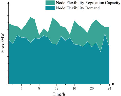
Figure 1. Illustration of flexibility coverage index

Where, ${FCI}_m$ represents the Flexibility Coverage Index.

Finally, the minimum value of the appropriate flexibility coverage index according to different risk preferences will be selected as the evaluation index of temporal flexibility, and it will be added as a constraint to the flexibility resource allocation optimization model.

3 Modeling of multi-type flexibility resource adjustment capacity

The considered flexibility resources in this study include thermal power units, solar-thermal power stations, and energy storage devices such as hydrogen storage, electrochemical storage, and pumped storage.

3.1 Thermal power units

Conventional thermal power units typically exhibit stable operating characteristics, providing continuous power output and meeting power demand over long time scales. Their advantages become more apparent, especially when dealing with significant fluctuations or long-term demands within the system. However, conventional thermal power units cannot achieve frequent charging and discharging in a short time, resulting in a slower response speed and insufficient flexibility when handling high-frequency but low-amplitude random fluctuations. The ramping performance, as well as the upper and lower limits of instantaneous output and output power, of conventional thermal power units affect their flexibility regulation capacity. Therefore, the flexibility of conventional thermal power plants on a time scale of $\Delta \mathrm{t}$ is as follows. The function is shown in Formula (11), (12).

$F_{G,∆t}^{+}=\mathit{min}\left(P_{G,\mathit{max}}-P_{G,t},R\bullet ∆t\right)(11)$

$F_{G,∆t}^{-}=\mathit{min}\left(P_{G,t}-P_{G,\mathit{min}},R\bullet ∆t\right)(12)$

Where, $P_{G,\mathit{max}}$, $P_{G,\mathit{min}}$, and $P_{G,t}$ represent the maximum, minimum, and current output of the unit at time t, respectively; $R$ is the ramping rate of the unit.

3.2 Solar-thermal power station

Solar-Thermal Power Stations typically have controllable thermal energy release characteristics, allowing adjustment of the energy release rate and duration according to the power system’s needs. This controllability enables them to flexibly participate in the power system’s response scheduling, providing power according to demand. Their flexibility for upward and downward adjustments on a time scale is shown in formula (13), (14).

$F_{csp,∆t}^{+}=\mathit{min}\left(P_{csp,\mathit{max}}^{+},\frac{\left(E_t-E_{\mathit{min}}+P_{SF-HTF}\bullet ∆t\right){\eta }_{RC}}{∆t}\right)(13)$

$F_{csp,∆t}^{-}=\mathit{min}\left(P_{csp,\mathit{max}}^{-},\frac{\left(E_{\mathit{max}}-E_t-P_{SF-HTF}\bullet ∆t\right){\eta }_{EH}}{∆t}\right)(14)$

Where, $P_{csp,\mathit{max}}^{+}$ and $P_{csp,\mathit{max}}^{-}$ are the maximum power generation and heat storage power of the solar-thermal power station, respectively; $E_t$, $E_{\mathit{max}}$, and $E_{\mathit{min}}$ are the upper and lower limits of the thermal storage capacity of the solar-thermal power station at time $t$; $P_{SF-HTF}$ is the thermal power collected by the solar field.

3.3 Energy storage devices

Energy storage devices not only serve as responsive power sources with excellent performance to meet large-scale, system-level applications on the grid side, but also provide bidirectional regulation flexibility by frequently converting electrical energy in a short time. This effectively handles high-frequency but low-amplitude random fluctuations.

Its upward and downward flexibility at time scale $\Delta \mathrm{t}$ is shown in formula (15), (16):

$\left.F_{es,∆t}^{+}=\mathit{min}\left(P_{es,\mathit{max}}^d-P_{es,t},\frac{\left.\left({SOC}_t-{SOC}_{\mathit{min}}\right){\eta }_{dis}-P_{es,t}∆t\right)}{∆t}\right.\right)(15)$

$\left.F_{es,∆t}^{+}=\mathit{min}\left(P_{es,\mathit{max}}^c+P_{es,t},\frac{\left.\left({SOC}_{\mathit{max}}-{SOC}_t\right)/{\eta }_{ch}+P_{es,t}∆t\right)}{∆t}\right.\right)(16)$

Where, $P_{es,\mathit{max}}^d$ and $P_{es,\mathit{max}}^c$ are the maximum discharge and charge power of the energy storage device, respectively; $P_{es,t}$ is the power at time t, positive for discharge and negative for charge; ${SOC}_t$, ${SOC}_{\mathit{max}}$, and ${SOC}_{\mathit{min}}$ are the upper and lower limits of the stored equivalent energy and device capacity at time t, respectively; ${\eta }_{dis}$ and ${\eta }_{ch}$ are the efficiency of discharge and charge.

The paper considers pumped storage power stations, hydrogen energy storage systems, and electrochemical energy storage as the main components for configuring energy storage devices. Among them, pumped storage units have strong capacity benefits, fast response rates, and deep response capabilities, effectively addressing peak shaving and valley filling of the net load; hydrogen energy storage systems store electrical energy on a large scale using hydrogen as a medium, which can also achieve peak shaving and valley filling of the net load. At the same time, they can respond rapidly to fluctuations in the net load. However, the current stage has a relatively low energy conversion efficiency. Electrochemical energy storage has an extremely high response rate, can smooth out high-frequency random fluctuations in the net load, but its installed capacity is limited by technical characteristics and cost factors, leading to limited response depth.

4 Two-stage optimization model for flexible resource configuration

4.1 Two-stage configuration optimization framework system

The paper first filters out nodes with insufficient flexibility based on spatial flexibility assessment indicators. Secondly, considering the constraints of temporal flexibility assessment indicators and the adjustment characteristics of flexibility resources at different time scales, different types of flexibility resources are phased in to meet the flexibility requirements of the power system at both long and short time scales. In the first phase, the focus is on configuring flexibility resources such as pumped storage power stations, solar-thermal power stations, and hydrogen energy storage systems with high adjustment depth and long duration to meet the requirements of long-time scale climbing or peak shaving and valley filling. In the second phase, the emphasis is on flexibility resources with extremely fast response rates, such as electrochemical energy storage, to cope with real-time high-frequency fluctuations in new energy and load. The two-stage framework for flexible resource allocation is shown in Figure 2.

Figure 2

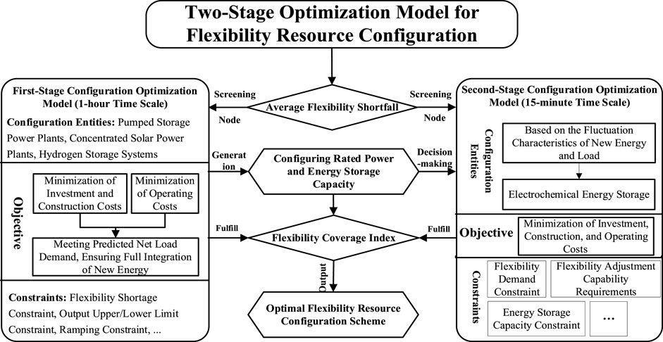
Figure 2. Two-stage framework for flexible resource allocation.

4.2 Two-stage configuration optimization model for flexibility resource

4.2.1 First stage configuration optimization model

In Stage 1, with a time scale of 1 h, it is mainly used to meet the forecast net load demand of each node, ensuring the full consumption of new energy. The objective function is to minimize the investment construction cost and operating cost. The function is shown in Formula (17).

$\begin{array}{c}\mathit{min}{C}_{cb,total}^m=C_{cb,inv}^m+C_{cb,cpe}^m\\ \left\{\begin{array}{c}{C}_{cb,inv}^m={\displaystyle \sum _{i\in N_{cb}}}\frac{r{\left(1+r\right)}^{y_i}}{{\left(1+r\right)}^{y_i}-1}\left(c_{cb,i}^P{P}_{cb,i,\mathit{max}}^m+c_{cb,i}^e{E}_{cb,i,\mathit{max}}^m\right)\\ C_{cb,cpe}^m={\displaystyle \sum _{i=1}^{T_1}}\left({\displaystyle \sum _{i\in N_{cb}}}{c}_{cb,i}^{ope}{P}_{cb,i,t}^m+{\displaystyle \sum _{k\in N_g}}{C}_{g,k,t}^m\right)\end{array}\right.\end{array}(17)$

Where, $C_{cb,total}^m$ is the total cost of flexibility resources for node $m$; $C_{cb,inv}^m$ and $C_{cb,cpe}^m$ are the investment construction cost and operating cost of flexibility resources for node $m$; $N_{cb}$ and $N_g$ are the sets of flexibility resources and conventional thermal power units configured in Stage 1; r is the discount rate; $y_i$ is the lifespan of the ith resource; $c_{cb,i}^P$ and $c_{cb,i}^e$ are the investment construction costs per unit rated power and unit storage capacity of the ith resource; $P_{cb,i,\mathit{max}}^m$ and $E_{cb,i,\mathit{max}}^m$ are the rated power and storage capacity of the ith resource at node $m$; $c_{cb,i}^{ope}$ is the cost of per unit operating power for the ith resource; $P_{cb,i,t}^m$ is the operating power of the ith resource at node $m$ in the timeslot $t$; $C_{g,k,t}^m$ is the operating cost of the ith conventional thermal power unit at node $m$ in the timeslot $k$.

Constraint conditions are as follows.

1) After configuring flexibility resources, it is necessary to meet the net load demands of nodes and ensure that no flexibility shortfall occurs. The function is shown in Formula (18).

${\displaystyle \sum _{i\in N_{cb}}}{P}_{cb,i,t}^m+{\displaystyle \sum _{k\in N_g}}{P}_{g,k,t}^m+{\displaystyle \sum _{n\in N_m}}{P}_{mn,t}=P_{net,t}^m+P_{ex,t}^m(18)$

Where, $P_{cb,i,t}^m$ and $P_{g,k,t}^m$ are the operating powers of the flexibility resource $i$ and conventional thermal power unit $k$ at node $m$ in timeslot $t$ during the first stage of configuration.

2) Pumped storage power stations and hydrogen energy storage systems, as energy storage devices, also need to satisfy the energy storage capacity constraints. The function is shown in Formula (19).

$\left\{\begin{array}{l}{E}_{cb,i,t}^m=E_{cb,i,t-1}^m+{\eta }_{cb,i}^{ch}{P}_{cb,i,t}^{m,ch}∆t-\frac{P_{cb,i,t}^{m,dis}∆t}{{\eta }_{cb,i}^{dis}}\\ 0\le E_{cb,i,t}^m\le E_{cb,i,\mathit{max}}^m\end{array}\right.(19)$

Where, $E_{cb,i,t}^m$ is the equivalent energy stored by the flexibility resource $i$ at node $m$ at timeslot $t$; ${\eta }_{cb,i}^{ch}$ and ${\eta }_{cb,i}^{dis}$ are the charging and discharging efficiencies of the flexibility resource $i$; $P_{cb,i,t}^{m,ch}$ and $P_{cb,i,t}^{m,dis}$ are the charging and discharging powers of the flexibility resource $i$ at node $m$ at timeslot $t$. The function is shown in Formula (20).

$\left\{\begin{array}{c}{P}_{cb,i,t}^{m,ch}=-\mathit{min}\left(P_{cb,i,t}^m,0\right)\\ P_{cb,i,t}^{m,dis}=\mathit{max}\left(P_{cb,i,t}^m,0\right)\end{array}\right.(20)$

Additionally, it is necessary to consider the output upper and lower limits, reserve output upper limits, ramping constraints, and rotating reserve constraints of flexibility resources and existing resources, which are not further elaborated here. The transmission power and reserve output between nodes $P_{mn,t}$, $R_{mn,t}^{up}$, $R_{mn,t}^{down}$ are the result values obtained from the optimized base output scenario in Section 2.2. Finally, $E_{cb,i,\mathit{max}}^m$ represents the configuration results of various types of flexibility resources obtained through optimization, and $P_{cb,i,t}^m$ will be passed as a parameter to the second-stage configuration optimization model.

4.2.2 Second stage configuration optimization model

The short-time scale configuration optimization model for stage 2, based on the initial output plan, generates a baseline output plan for a 15-min time scale. Subsequently, it optimizes the configuration of units with fast regulation rates according to the fluctuation characteristics of new energy and load. The objective function is to minimize the total investment and operating costs, and it is represented in formula (21).

$\begin{array}{c}\mathit{min}{C}_{fm,total}^m=C_{fm,inv}^m+C_{fm,ope}^m\\ \left\{\begin{array}{l}{C}_{fm,inv}^m={\displaystyle \sum _{i\in N_{fm}}}\frac{r{\left(1+r\right)}^{y_j}}{{\left(1+r\right)}^{y_j}-1}\left(c_{fm,j}^P{P}_{fm,j,\mathit{max}}^m+c_{fm,j}^e{E}_{fm,j,\mathit{max}}^m\right)\\ C_{fm,ope}^m={\displaystyle \sum _{t=1}^{T_2}}\left({\displaystyle \sum _{j\in N_{fm}}}{c}_{fm,j}^{ope}{P}_{fm,j,t}^m+{\displaystyle \sum _{i\in N_{cb}}}{c}_{cb,i}^{ope}∆P_{cb,i,t}^m\right)\end{array}\right.\end{array}(21)$

Where, $C_{fm,total}^m$ is the total cost of flexibility resources for node $m$; $C_{fm,inv}^m$ and $C_{fm,ope}^m$ are the investment construction cost and operating cost of flexibility resources for node $m$; $N_{fm}$ is the set of electrochemical energy storage units; other variables are consistent with the flexibility resource configuration optimization model in Stage 1, which is not repeated here. $P_{fm,j,\mathit{max}}^m$ and $E_{fm,j,\mathit{max}}^m$ are the optimized configuration results of electrochemical energy storage units.

Constraint conditions are as follows.

1) Some of the flexibility resources configured in Stage 1 can also provide a certain degree of regulation capability, and both need to meet the flexibility requirements at a 15-min time scale, it is represented in formula (22).

$\left\{\begin{array}{l}{\displaystyle \sum _{j\in N_{fm}}}{P}_{fm,j,t}^m+{\displaystyle \sum _{i\in N_{cb}}}∆P_{cb,i,t}^m={\delta }_{m,t}^{net}\\ ∆P_{cb,i,t}^m=P_{cb,i,t}^m-P_{cb,i,t-1}^m\end{array}\right.(22)$

Where, $P_{fm,j,t}^m$ represents the operating power of the flexibility resource $j$ configured at node $m$ in Stage 2 at time $t$; $∆P_{cb,i,t}^m$ represents the power variation of the flexibility resource i configured at node $m$ in Stage 1 at time $t$, which still needs to satisfy the output upper limit constraint and ramping constraint of the flexibility resource. Pumped storage and hydrogen storage systems also need to meet the energy storage capacity constraint, which is not elaborated here; ${\delta }_{m,t}^{net}$ represents the fluctuation characteristics of the net load at a 15-min time scale, which can be derived from historical data for convenience.

2) The flexibility adjustment capability of each node at a 15-min time scale needs to be greater than the stochastic fluctuations of wind power, photovoltaics, and load at the same time scale. The function is shown in Formula (23).

$\left\{\begin{array}{c}{F}_{up,t}^m={\displaystyle \sum _{j\in N_{fm}}}{F}_{fm,j,t}^{m,up}+{\displaystyle \sum _{i\in N_{cb}}}{F}_{cb,i,t}^{m,up}\ge {\beta }_{wpp}{P}_{wpp,t}^m+{\beta }_{pv}{P}_{pv,t}^m+{\beta }_{load}{P}_{load,t}^m\\ F_{dn,t}^m={\displaystyle \sum _{j\in N_{fm}}}{F}_{fm,j,t}^{m,dn}+{\displaystyle \sum _{i\in N_{cb}}}{F}_{cb,i,t}^{m,dn}\ge {\beta }_{wpp}{P}_{wpp,t}^m+{\beta }_{pv}{P}_{pv,t}^m+{\beta }_{load}{P}_{load,t}^m\end{array}\right.(23)$

Where, $F_{up,t}^m$ and $F_{dn,t}^m$ represent the upward/downward flexibility adjustment capabilities of node $m$ at time $t$; $F_{fm,j,t}^{m,up}$ and $F_{fm,j,t}^{m,dn}$ represent the upward/downward flexibility adjustment capabilities of flexibility resource $j$ configured in Stage 2 at time $t$; $F_{cb,i,t}^{m,up}$ and $F_{cb,i,t}^{m,dn}$ represent the upward/downward flexibility adjustment capabilities of flexibility resource i configured in Stage 1 at time t; ${\beta }_{wpp}$, ${\beta }_{pv}$ and ${\beta }_{load}$ are the random fluctuation coefficients of wind power, photovoltaics, and load at a 15-min time scale, respectively.

3) Flexibility resources need to satisfy output upper and lower limits, ramping constraints, and electrochemical energy storage also needs to consider energy storage capacity constraints; this is not reiterated here.

4) In order to enhance the system’s ability to cope with the random fluctuations of new energy/load, the optimization models for flexibility resource configuration in both stages need to satisfy flexibility indicator constraints. The function is shown in Formula (24).

$\left\{\begin{array}{c}{FCI}_{m,s}^{up}\ge {\epsilon }_{FIC,s}^{up}\\ {FCI}_{m,s}^{down}\ge {\epsilon }_{FIC,s}^{down}\end{array}\right.,s\in S(24)$

Where, $S$ represents the set of considered time scales, including the 1-h time scale and the 15-min time scale; ${\epsilon }_{FIC,s}^{up}$ and ${\epsilon }_{FIC,s}^{down}$ are the thresholds set for the flexibility coverage index at scale s, which is typically chosen between one and 1.2. The specific values of the time flexibility indicator thresholds depend on the decision-maker’s requirements for system reliability and flexibility.

4.3 Solution procedure

The method for configuring multiple types of flexibility resources, considering spatiotemporal response characteristics, is illustrated in Figure 3. The steps for solving are as follows:

1) Obtain information about the system’s network structure, current resource configuration, node net load forecasts, resource technical parameters, etc.

2) Utilize the flexibility evaluation model based on spatial response characteristics to generate baseline output plans for each node. Calculate the spatial flexibility indicators for each node to determine the node type. If the indicator value for a node is less than the threshold, it is classified as a node with sufficient flexibility; otherwise, it is classified as a node with insufficient flexibility.

3) Based on the multiscale matching characteristics of multiple types of flexibility resources and the fluctuation characteristics of new energy sources, construct an optimization model for flexibility resource capacity configuration. Use the flexibility evaluation model based on temporal response characteristics to guide the formation of flexibility resource configuration schemes that consider time flexibility constraints.

Figure 3

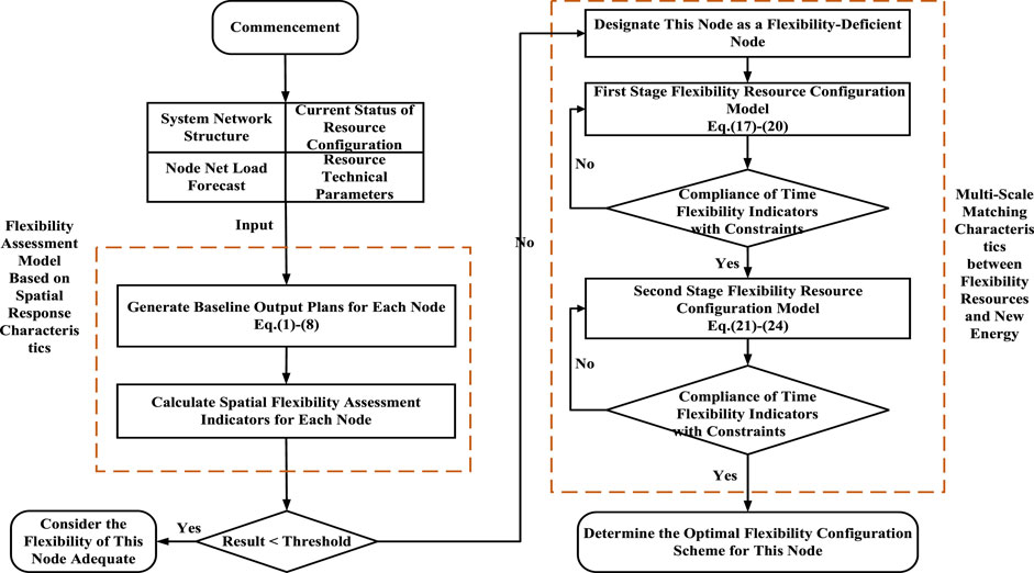
Figure 3. Flowchart of flexible resource configuration steps.

5 Example analysis

5.1 Example data

In order to simplify the computational complexity and save the simulation computation time, this paper adopts the IEEE 9-node network system shown in Figure 4 for the simulation analysis, and performs the arithmetic simulation on matlab R2022a, and calls the cplex solver through the yalmip toolbox to solve the model, so as to validate the validity and applicability of the flexibility resource allocation method proposed in this paper. Theoretically, the number of nodes can be expanded as needed to accommodate larger systems. In this case, the data for the whole year is scaled by a suitable ratio to obtain the data of wind power output, photovoltaic output and load level at each node for the whole year of 365 × 24 h. Due to the extremely uneven distribution of energy resources and energy demand market in China, the system considers the situation of power transmission. In order to give full play to the renewable energy supply potential in the region, a larger regional power outflow demand is set. The power outgoing demand in one dispatching cycle is shown in Figure 5.

Figure 4

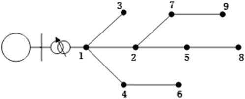
Figure 4. IEEE 9-node network diagram.

Figure 5

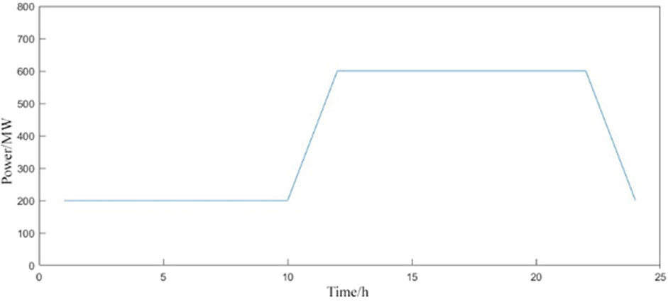
Figure 5. Electricity export demand chart.

In addition, the current installed capacity of new energy sources and the configuration status of flexibility resources for each node are presented in Table 1. Currently, only thermal power units and hydropower units are used for flexibility adjustment. Since Nodes 4, 8, and 9 do not have hydropower units, it is assumed in this paper that these nodes have relatively scarce water resources and cannot configure pumped storage units. The cost parameters for different types of flexibility resources are outlined in Table 2.

Table 1

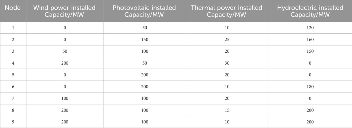
Table 1. Current status of new energy installations and flexible resource allocation at each node.

Table 2

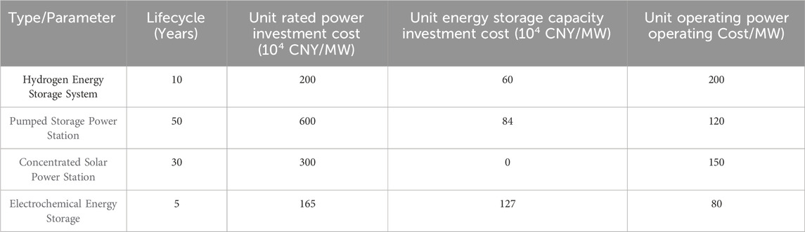
Table 2. Cost parameters for various types of flexible resources.

5.2 Example result

This paper mainly considers four types of flexibility resources: solar-thermal, pumped storage, hydrogen storage systems, and electrochemical energy storage. Solar-thermal, pumped storage, and hydrogen storage systems are considered as the initial stage configuration flexibility resources, while electrochemical energy storage is considered as the adjustment stage configuration flexibility resource.

Firstly, using the flexibility assessment model based on spatial response characteristics in Section 1.2, the current flexibility deficits for each node are obtained, and nodes with insufficient flexibility are identified. The flexibility deficits in each time period of the scheduling cycle are shown in Figure 5. The mutual support of electrical energy and flexibility between nodes is illustrated in Figure 6.

Figure 6

Figure 6. Flexibility deficit chart for each node within the scheduling period.

Combining Figure 6 and Figure 7, it is evident that there is no upward flexibility deficit in the system. However, all nodes except Node four experience downward flexibility deficits, concentrated in the time period from 10 to 14. Nodes such as 3, 8, and 9 have abundant hydroelectric resources, resulting in surplus flexibility adjustment capabilities. These nodes will provide some upward and downward reserves through regional power grid support for other nodes. Based on this, the average flexibility deficit and spatial flexibility index for each node are calculated, with results presented in Table 3.

Figure 7

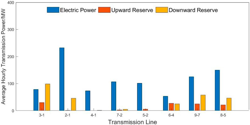
Figure 7. Electricity and flexibility transfer diagram among nodes.

Table 3

Table 3. Average flexibility deficit across nodes.

Assuming the threshold for the average flexibility deficit at each node is set to 2 MW/h, nodes with insufficient flexibility, namely, 2, 5, 6, 7, 8, and 9, are filtered. Subsequently, a two-stage configuration optimization model is employed to allocate the required types of flexibility resources for each node. The flexibility coverage index thresholds for Stage 1 and Stage 2 of the flexibility resource allocation optimization model are set to 1.05 and 1.1, respectively. The optimized flexibility resource allocation results for each node are presented in Figure 8, and the corresponding investment and construction costs as well as operating costs are detailed in Table 4.

Figure 8

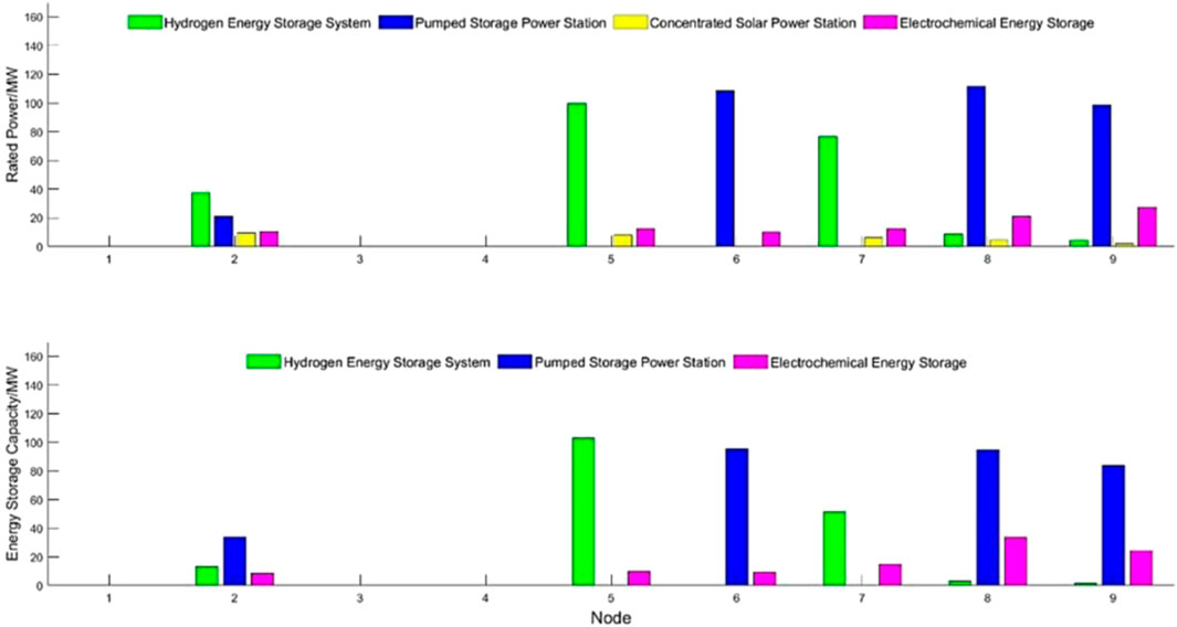
Figure 8. Optimization results for flexible resource allocation at each node.

Table 4

Table 4. Investment and operating costs for each node.

From Figure 8, it can be observed that due to the ability of hydrogen storage systems and pumped storage power stations to store a large amount of electrical energy while also considering economic factors, when the flexibility deficit is significant, nodes will prioritize the configuration of pumped storage power stations. Nodes that cannot configure pumped storage power stations will choose to configure hydrogen storage systems. Although solar-thermal power stations have a certain degree of flexibility, they are still limited by sunlight conditions. Therefore, their regulation capabilities are affected during nighttime or cloudy weather, making them somewhat limited, with smaller configuration capacities at each node. Additionally, to mitigate the stochastic fluctuations of net load on shorter time scales, nodes will configure a certain capacity of electrochemical energy storage, and the configuration capacity will increase with the increase in the installed capacity of renewable energy sources in the region where the node is located.

Next, the flexibility coverage index threshold is set to 1, 1.05, 1.1, 1.15, and 1.2, respectively. The total investment and construction costs, as well as operating costs, for configuring electrochemical energy storage at each node in Phase 2 are calculated and presented in Table 5, and the configuration optimization results are shown in Figure 9. The configuration results are analyzed based on the threshold of 1.1, and the relative changes in the configured node energy storage capacity are depicted in Figure 10.

Table 5

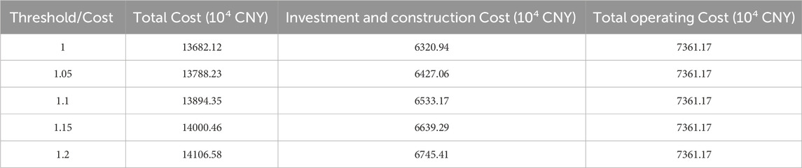
Table 5. Total investment and operating costs for node system in stage 2.

Figure 9

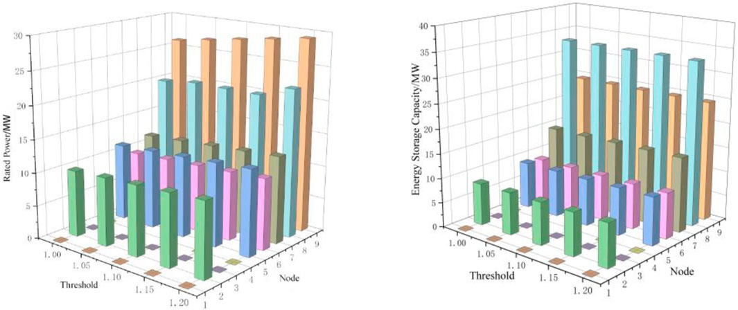
Figure 9. Optimization results for flexible resource allocation at each node in stage 2 under different thresholds.

Figure 10

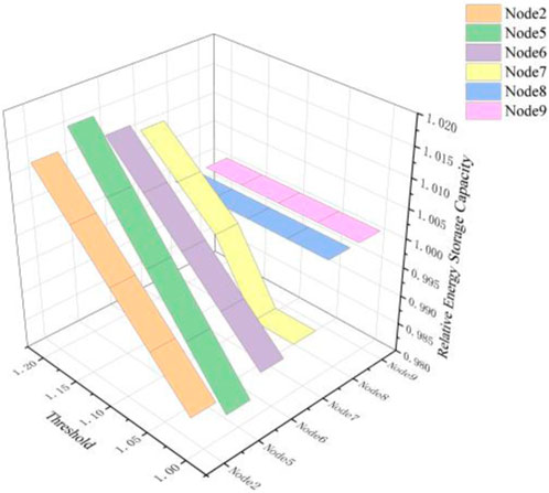
Figure 10. The relative energy storage capacity of flexibility resources allocated to nodes in stage 2 at different thresholds.

From Table 5, it can be observed that with the increase in the flexibility coverage index threshold, the total investment and construction costs continuously increase, while the total operating costs remain constant. This is because, with the increase in the threshold, the requirement for reserve resources to better cope with the uncertainty of load and wind-solar output increases, necessitating the expansion of reserve capacity, thus increasing the overall construction costs. As for operating costs, they are only related to the operating power of resources and the unit operating cost, independent of changes in the configuration of reserve capacity. Therefore, regardless of how the configuration is altered, operating costs remain constant.

6 Conclusion

To enhance the safety and reliability of future renewable energy power systems, this paper proposes a spatiotemporal response-aware multi-type flexibility resource configuration optimization model. Considering the regulating characteristics of various flexibility resources, the paper optimizes the configuration of flexibility resources in the power system to obtain an optimal planning solution. Simulation results indicate:

1) Based on the set average flexibility deficit indicator method, this paper conducts a spatial flexibility assessment, allowing system operators or planners to concentrate resources and attention on nodes that most require additional flexibility resources. This targeted approach facilitates the allocation of appropriate types of flexibility resources to specific nodes.

2) The two-stage configuration optimization model for flexibility resource capacity proposed in this paper, by considering the different regulation characteristics and mutual cooperation of multiple types of flexibility resources, enables flexible decision-making. This phased configuration of flexibility resources helps the power system better accommodate and integrate new energy, reducing dependence on traditional fossil fuels.

3) The proposed flexibility coverage index threshold in this paper can effectively guide the flexibility resource allocation schemes for nodes with insufficient flexibility. Additionally, as the flexibility coverage index threshold increases, the requirements for the capacity of flexibility resource allocation increase, leading to an overall increase in investment and construction costs.

Data availability statement

The original contributions presented in the study are included in the article/Supplementary materials, further inquiries can be directed to the corresponding author.

Author contributions

YL: Conceptualization, Methodology, Validation, Writing–original draft, Conceptualization, Methodology, Validation, Writing–original draft, MZ: Visualization, Writing–review and editing, Visualization, Writing–review and editing.

Funding

The author(s) declare that financial support was received for the research, authorship, and/or publication of this article. This work is supported by Science and Technology Project of Shanxi Electric Power Company (520533230006).

Acknowledgments

We would like to thank Shanxi Electric Power Company for their help in the design of our study.

Conflict of interest

Author YL was employed by Economic and Technical Research Institute of Shanxi Electrical Power Company of SGCC.

The remaining authors declare that the research was conducted in the absence of any commercial or financial relationships that could be construed as a potential conflict of interest.

The authors declare that this study received funding from Science and Technology Project of Shanxi Electric Power Company. The funder had the following involvement in the study: design of our study.

Publisher’s note

All claims expressed in this article are solely those of the authors and do not necessarily represent those of their affiliated organizations, or those of the publisher, the editors and the reviewers. Any product that may be evaluated in this article, or claim that may be made by its manufacturer, is not guaranteed or endorsed by the publisher.

References

Clegg, S., and Mancarella, P. (2016). Integrated electrical and gas network flexibility assessment in low-carbon multi-energy systems. IEEE Trans. Sustain. Energy 7 (2), 718–731. doi:10.1109/tste.2015.2497329

CrossRef Full Text | Google Scholar

Degefa, M. Z., Sperstad, I. B., and Sæle, H. (2021). Comprehensive classifications and characterizations of power system flexibility resources. Electr. Power Syst. Res. 194, 107022. doi:10.1016/j.epsr.2021.107022

CrossRef Full Text | Google Scholar

Guo, Z., Zheng, Y., and Li, G. (2020). Power system flexibility quantitative evaluation based on improved universal generating function method: a case study of Zhangjiakou. Energy 205, 117963. doi:10.1016/j.energy.2020.117963

CrossRef Full Text | Google Scholar

Hong, TANG, Wang, S., and Hangxin, L. I. (2021). Flexibility categorization, sources, capabilities and technologies for energy-flexible and grid-responsive buildings: state-of-the-art and future perspective. Energy 219, 119598. doi:10.1016/j.energy.2020.119598

CrossRef Full Text | Google Scholar

Huang, Y., Kuldasheva, Z., Bobojanov, S., Djalilov, B., Salahodjaev, R., and Abbas, S. (2023). Exploring the links between fossil fuel energy consumption, industrial value-added, and carbon emissions in G20 countries. Environ. Sci. Pollut. Res. 30 (4), 10854–10866. doi:10.1007/s11356-022-22605-9

CrossRef Full Text | Google Scholar

Ji, L., Wu, Y., Liu, Y., Sun, L., Xie, Y., and Huang, G. (2022). Optimizing design and performance assessment of a community-scale hybrid power system with distributed renewable energy and flexible demand response. Sustain. Cities Soc. 84, 104042. doi:10.1016/j.scs.2022.104042

CrossRef Full Text | Google Scholar

Jiawei, FENG, Yang, J., Wang, H., Ji, H., Okoye, M. O., Cui, J., et al. (2020). Optimal dispatch of high-penetration renewable energy integrated power system based on flexible resources. Energies 13 (13), 3456. doi:10.3390/en13133456

CrossRef Full Text | Google Scholar

Jie, JIAN, Peng, L. I., Haoran, J. I., Bai, L., Yu, H., Xi, W., et al. (2022). DLMP-based quantification and analysis method of operational flexibility in flexible distribution networks. IEEE Trans. Sustain. Energy 13 (4), 2353–2369. doi:10.1109/tste.2022.3197175

CrossRef Full Text | Google Scholar

Li, H., Zhang, N., Bao, W., et al. (2022). Modeling and planning of multi-timescale flexible resources in power systems. CSEE J. Power Energy Syst., 1–10. doi:10.17775/CSEEJPES.2021.04850

CrossRef Full Text | Google Scholar

Lu, Z., Li, H., and Qiao, Y. (2018). Probabilistic flexibility evaluation for power system planning considering its association with renewable power curtailment. IEEE Trans. Power Syst. 33 (3), 3285–3295. doi:10.1109/tpwrs.2018.2810091

CrossRef Full Text | Google Scholar

Ren, Z., Guo, H., Yang, P., Zuo, G., and Zhao, Z. (2020). Bi-level optimal allocation of flexible resources for distribution network considering different energy storage operation strategies in electricity market. IEEE Access 8, 58497–58508. doi:10.1109/access.2020.2983042

CrossRef Full Text | Google Scholar

Ren, Z., Guo, H., Yang, P., Zuo, G., and Zhao, Z. (2020a). Bi-level optimal allocation of flexible resources for distribution network considering different energy storage operation strategies in electricity market. IEEE Access 8, 58497–58508. doi:10.1109/access.2020.2983042

CrossRef Full Text | Google Scholar

Ren, Z., Guo, H., Yang, P., Zuo, G., and Zhao, Z. (2020b). Bi-level optimal allocation of flexible resources for distribution network considering different energy storage operation strategies in electricity market. IEEE Access 8, 58497–58508. doi:10.1109/access.2020.2983042

CrossRef Full Text | Google Scholar

Tang, X., Hu, Y., Chen, Z., and You, G. (2020). Flexibility evaluation method of power systems with high proportion renewable energy based on typical operation scenarios. Electronics 9 (4), 627. doi:10.3390/electronics9040627

CrossRef Full Text | Google Scholar

Ting, Z., and Yunna, W. (2024). Collaborative allocation model and balanced interaction strategy of multi flexible resources in the new power system based on Stackelberg game theory. Renew. Energy 220, 119714. doi:10.1016/j.renene.2023.119714

CrossRef Full Text | Google Scholar

Turk, A., Wu, Q., Zhang, M., and Østergaard, J. (2020). Day-ahead stochastic scheduling of integrated multi-energy system for flexibility synergy and uncertainty balancing. Energy 196, 117130. doi:10.1016/j.energy.2020.117130

CrossRef Full Text | Google Scholar

Xiaowei, Y. U., Xu, LING, Xiaogang, ZHOU, Li, K., and Feng, X. (2022). Flexibility evaluation and index analysis of distributed generation planning for grid-source coordination. Front. Energy Res. 10. doi:10.3389/fenrg.2022.1019352

CrossRef Full Text | Google Scholar

Yan, X., Jiang, H., Gao, Y., Li, J., and Abbes, D. (2020). “Practical flexibility analysis on europe power system with high penetration of variable renewable energy,” in 2020 IEEE Sustainable Power and Energy Conference (iSPEC), Chengdu, China, November, 2020, 395–402. doi:10.1109/ispec50848.2020.9351168

CrossRef Full Text | Google Scholar

Yang, H., Tian, X., Liu, F., Liu, L., Li, L., and Wang, Q. (2023). A multi-objective dispatching model for a novel virtual power plant considering combined heat and power units, carbon recycling utilization and flexible load response. Front. Energy Res. 11, 1332474. doi:10.3389/fenrg.2023.1332474

CrossRef Full Text | Google Scholar

Zhang, T., Ma, Y., Wu, Y., and Yi, L. (2023). Optimization configuration and application value assessment modeling of hybrid energy storage in the new power system with multi-flexible resources coupling. J. Energy Storage 62, 106876. doi:10.1016/j.est.2023.106876

CrossRef Full Text | Google Scholar

Zhijie, L. I. U., Zhu, S., Zhang, P., and Zhang, Z. (2022). “Flexibility evaluation index system and calculation method of active distribution network with high proportion of renewable energy,” in 2022 Asian Conference on Frontiers of Power and Energy (ACFPE), Chengdu, China, October, 2022, 720–724. doi:10.1109/acfpe56003.2022.9952278

CrossRef Full Text | Google Scholar