Multivariate low-carbon scheduling of distribution network based on improved dynamic carbon emission factor

The “load-following” characteristic of the power system makes the electricity consumption behavior on the load side crucial for the low-carbon operation of the distribution network. To address this, this paper proposes an improved dynamic carbon emission factor for the distribution network, taking into account the spatiotemporal characteristics of carbon emission intensity and the integration capacity of photovoltaics (PV). Based on this, a calculation method for the carbon emissions of the distribution network load is provided. Subsequently, for commercial and industrial user scenarios, demand response models are separately constructed for commercial and industrial loads based on different driving mechanisms. Using time-of-use electricity prices as decision variables, optimization scheduling of the distribution network is carried out with the objectives of minimizing scheduling costs and carbon emissions. At the same time, a case study is conducted in an improved IEEE-33 node distribution network. The results indicate that, under the guidance of the improved dynamic carbon emission factor, load transfer can be achieved through fluctuating electricity prices, effectively reducing the scheduling costs of the distribution network, decreasing carbon emissions, and enhancing the PV integration capacity of the distribution network in different user scenarios. Finally, it is hoped that in the future, this optimization method can be widely applied, and further research can explore coordinated strategies among generation, network, load, and storage to advance the development of the power industry.

1 Introduction

Since the proposal of the Dual Carbon Goals by the 75th United Nations General Assembly in September 2020, various industries have been continuously moving towards the direction of green and low-carbon initiatives. As a crucial infrastructure supporting modern society, the power system plays a key role in achieving low-carbon emission objectives. The distribution network, being the end of the power system and connected to end-users, has a direct and far-reaching impact on carbon emission levels through its scheduling methods and topological structure (Kang et al., 2009). Therefore, it is an urgent task to develop rational optimization and scheduling plans, considering the carbon emission characteristics of different loads in the distribution network, to reduce carbon emissions while ensuring the economic operation of the distribution network.

In recent years, research on carbon emissions in power systems has shifted from generation to the load side. Although carbon emissions primarily originate from the generation side, distributed generation units on the distribution network side have almost zero carbon emissions. However, due to the diversity and uncertainty of distribution network loads, changes in load flow will occur, and carbon flow is dependent on the existence of load flow. The introduction of different loads will change the carbon emission intensity of the distribution network. Therefore, considering the carbon emission flow theory (Zhou et al., 2012), research on the low-carbon optimization operation of distribution networks under different scenarios is conducted. The distribution characteristics of carbon emission flow in distribution systems developed by (Zhou and Kang, 2019) and establishes a carbon emission flow calculation model for energy storage components, proposing an optimization method for the operation of distribution systems towards low-carbon goals. The responsibility of carbon emissions shifts from the generation side to the load side and considers low-carbon optimization scheduling (Ge et al., 2023) based on carbon emission flow theory and demand response using carbon prices as a pricing signal, providing new insights for reducing system carbon emissions. (Zhang et al., 2023) addresses the issue of a singular low-carbon means on the load side in low-carbon scheduling and proposes a two-layer low-carbon economic scheduling model for power systems considering multiple carbon reduction methods coupled with the carbon potential of sources and loads. All of these studies introduce the theory of carbon emission flow into the power system, guiding electricity use for different types of users based on their electricity consumption characteristics but without optimizing considerations for load response characteristics and flexibility.

From the perspective of demand response, the optimization scheduling of flexible loads has gradually become a research focus for reducing carbon emissions. Considering the carbon emission characteristics of thermal power units and cement factories (Han et al., 2023), which proposed environmentally economic scheduling of typical industrial loads with positive demand response. Literature (Li et al., 2022a; Ibrahim et al., 2023) introduces a new mechanism for reducing carbon emissions in power systems by guiding users to respond actively, taking into account the users’ own carbon reduction intentions or the price factors in the carbon market as incentive signals. A distributed resource low-carbon scheduling strategy for distribution networks based on the carbon potential of nodes, considering both the economic and low-carbon aspects of power grid operations proposed in (Xue et al., 2019; Song et al., 2023a). The above studies on demand response in power systems do not take into account the impact of abandoned wind and solar power on the carbon emissions of distribution networks, as well as the differences in carbon emissions due to electricity consumption at different times.

In summary, based on the carbon emission flow theory, this paper proposes an improved dynamic carbon emission factor calculation method considering temporal and spatial characteristics and the integration capacity of new energy sources. For different user scenarios, demand response models for commercial and industrial loads with the objectives of minimizing scheduling costs and carbon emissions are separately established. Finally, a case study is conducted on an IEEE-33 node distribution network, validating that the proposed model can effectively shift high-carbon emission periods to low-carbon emission periods in different scenarios while enhancing the photovoltaic integration capacity of the distribution network.

2 Calculation method for carbon emissions in distribution networks

2.1 Improved dynamic carbon emission coefficient for distribution networks

The traditional quantification of carbon emission levels in distribution networks mainly relies on the nodal carbon potential of the system. For a specific node, it is described as the ratio of the carbon flow into that node to its active power. Physically, it represents the carbon emission per unit of electricity consumed at the node, corresponding to the carbon emission density of the generator at that node and the weighted average of the carbon flow densities of adjacent nodes concerning the injected power from generators and adjacent nodes. The unit is kgCO₂/kW·h (Zhou et al., 2012) Eq. 1.

$e_j=\frac{{\displaystyle \sum _{j=1}^N}{P}_j\cdot {\rho }_j+P_{G,j}\cdot {\rho }_{G,j}}{{\displaystyle \sum _{j=1}^N}{P}_j+P_{G,j}}(1)$

In the equation, e_j represents the carbon potential of Node j, P_j represents Injected power at node j, P_G,j represents the injected power from generator units connected to node j, ρ_j represents the carbon flow density at node j, ρ_G,j represents the carbon potential of generatorn units connected to node j.

The traditional calculation for dynamic carbon emission factor in distribution networks is as follow Eq. 2 (Zhou and Kang, 2019):

$C_{Dis,t}=\frac{{\displaystyle \sum _{j=1,t\in T}^N}{P}_{j,t}\times e_{j,t}}{{\displaystyle \sum _{j=1,t\in T}^N}{P}_{j,t}}(2)$

In the equation, C_Dis,t represents the dynamic carbon emission factor of the urban distribution network at time t, P_j,t represents the active load magnitude of node t at time t, e_j,t represents the carbon potential magnitude of node t at time t, calculated based on the carbon emission flow theory, N represents the set of nodes within the distribution network.

The traditional dynamic carbon emission factor for distribution networks reflects the carbon emissions per unit of electricity consumption at time t. However, the improved dynamic carbon emission factor takes into account the equivalent carbon emissions generated by adding new energy sources. During these times, all electricity consumption in the distribution network comes from photovoltaic output, resulting in a dynamic carbon emission factor of zero for the distribution network. In such cases, users, when considering changes in their electricity consumption based on the dynamic carbon emission factor, cannot perceive the curtailed solar power at the moment when the carbon emission factor is zero. The closer its value is to zero, the higher the level of new energy consumption. Therefore, the equivalent reduction in carbon emissions is also different in article (Ge et al., 2022). The improved expression for the calculation of the dynamic carbon emission factor is as follows:

$\overline{C_{Dis,t}}=\frac{{\displaystyle \sum _{j=1,t\in T}^N}{P}_{j,t}\times e_{j,t}-P_{Q,t}\times e_{0,t}}{{\displaystyle \sum _{j=1,t\in T}^N}{P}_{j,t}}(3)$

In the equation, $\overline{C_{Dis,t}}$ represents the improved dynamic carbon emission factor for the distribution network, considering the curtailed solar power, P_Q,t represents the curtailed solar power in the distribution network at time t, e_0,t represents the carbon potential of the main grid at time t.

2.2 Calculation of carbon emissions in distribution networks

Based on the carbon potential matrix E formed by the carbon potential at each node in the distribution network and the active power flow matrix at load nodes, the carbon emissions at the load nodes can be determined, clearly defining the carbon emission responsibilities of different nodes.

The active power flow matrix at a specific node can be defined as a diagonal matrix, as shown below:

$P=\left(\begin{array}{ccc}{P}_{11}& 0& 0\\ 0& \ddots & 0\\ 0& 0& P_{nn}\end{array}\right)(4)$

Since there are no losses in the active power transmission between nodes, the off-diagonal elements are 0, the calculation for the diagonal elements is as follows Eq. 5 (Chen et al., 2023):

$P_{jj}=\left\{\begin{array}{l}{\displaystyle \sum _{l\in N^{+}}}{P}_l,l\notin k^{+}\\ {\displaystyle \sum _{l\in N^{+}}}{P}_l+P_{G,l},l\in k^{+}\end{array}\right.(5)$

In the equation,k⁺ represents the set of branches connected to node j that are adjacent and have generating units with power output, when a specific node is not adjacent to any generating units, that is $l\notin k$, the diagonal elements of the active power flow matrix P_jj is the active power flow entering node j; when there is a generating unit on a specific branch, then the diagonal element of the node adjacent to that branch P_jj is the sum of active power flow entering node j and the outputs of generating units connected to that node.

Combining (Eqs. 3, 4), the calculation method for the node carbon potential matrix is as follows for (Chen et al., 2023) Eq. 6:

$E={\left(P-P_B^T\right)}^{-1}{P}_{G,in}^T{Q}_G(6)$

In the equation, E represents the node carbon potential matrix, P_B represents the matrix of branch flow distribution, $P_{G,in}^T$ represents the matrix of generating unit injection flow distribution, Q_G the matrix of carbon emission intensity for generating units.

In distribution networks with a high proportion of photovoltaics, the carbon potential at a node is affected by both photovoltaic power sources and energy storage elements in discharge mode. If the distribution network lacks generating units and energy storage components, then in such a scenario, the carbon potential at all nodes equals the carbon potential of the main network. However, if the distribution network includes generating units and energy storage components, given the main network’s carbon potential, distribution network load, and generating unit outputs, it becomes possible to calculate the distribution of branch power flows and branch carbon flow density. Subsequently, node carbon potentials can be determined based on the carbon flow density of the branches.

If the dynamic carbon emission factor matrix $C_T=\left[C_{Dis,1},C_{Dis,2,},...,C_{Dis,T}\right]$ for the given time period T is provided, the improved dynamic carbon emission factor matrix for the system $\overline{C_T}=\left[\overline{C_{Dis,1}},\overline{C_{Dis,2}},...,\overline{C_{Dis,T}}\right]$, combining the matrix of active power load for the system $P_{L,t}=\left[P_{L,1},P_{L,2},...,P_{L,T}\right]$, the total carbon emissions R_T for the entire distribution network during that time period can be obtained as follow:

$R_T=\overline{C_T}\cdot P_{L,t}^T\cdot \Delta T(7)$

3 Demand response load model in distribution network

3.1 Incentive-based demand response

Traditional incentive-based demand response (Xu and Guo, 2023) mainly involves users adjusting or reducing electricity consumption during peak demand periods to receive discounts or compensation. This paper proposes an incentive-based demand response load considering the dynamic carbon emission factor. In this approach, agreements are pre-signed between the power supplier and the consumer. The dispatch center issues instructions the day before the demand response, and based on the dynamic carbon emission factor, the load is transferred from high carbon periods to low carbon periods. The load remains unchanged during neutral carbon periods. According to the agreement, users receive compensation after load transfer. The expression for compensation is as follows for Eq. 8 (Ge et al., 2022):

$\left\{\begin{array}{l}{W}_{IDR}^{ind}={\displaystyle \sum _{t=1}^N}{\beta }^{ind}{P}_{in,t}^{ind}={\displaystyle \sum _{t=1}^N}{\beta }^{ind}{P}_{out,t}^{ind}\\ W_{DRE}^{comp}={\displaystyle \sum _{t=1}^N}{\gamma }^{comp}{P}_{out,t}^{comp}\end{array}\right.(8)$

In the equation, $W_{IDR}^{ind}$ represents compensation for incentive-based load, ${\beta }^{ind}$ represents compensation coefficient for transferable load, $P_{in,t}^{ind}$ represents the amount of load transferred in at time t, $P_{out,t}^{ind}$ represents the amount of load transferred out at time t, $W_{DRE}^{comp}$ represents compensation for reducible load, ${\gamma }^{comp}$ represents compensation coefficient for reducible load, $P_{out,t}^{comp}$ represents the amount of load reduction at time t.

3.2 Price-based demand response

Price-based demand response in (Li et al., 2023) involves changing the original electricity consumption behavior based on changes in electricity prices. It mainly includes two methods: time-of-use pricing demand response and tiered pricing demand response. This paper primarily adopts time-of-use pricing demand response, aiming to improve the economic and low-carbon performance of the distribution network by responding to variations in electricity prices.

For electricity consumption periods under different carbon emission intensities, users will adjust their electricity consumption structure (Kaile et al., 2020). The electricity price level will not only affect the load of that period, but also affect the load of other periods, which is a multi period demand response. Based on the relationship between electricity quantity and price demand balance, and the multi-period electricity quantity-price elasticity matrix, users’ response behavior can be comprehensively characterized. The ratio of electricity quantity to price change rate can be described as the electricity quantity-price elasticity matrix, representing the sensitivity of electricity consumption in each period to prices. The expression is as follows for Eq. 9 (Zhou et al., 2016):

$\chi =\frac{\Delta E}{\Delta P}\cdot \frac{P}{E}(9)$

In the equation, $\chi$ represents electricity quantity-price elasticity indicator, E and $\Delta E$ the quantity of electricity and its variation respectively, P and $\Delta P$ represent the price and its variation respectively.

The expression for the electricity quantity-price elasticity matrix M under time-of-use pricing is Eq. 10 (Zhou et al., 2016):

$M=\left[\begin{array}{ccc}{\delta }_{hh}& {\delta }_{hm}& {\delta }_{hl}\\ {\delta }_{mh}& {\delta }_{mm}& {\delta }_{ml}\\ {\delta }_{lh}& {\delta }_{lm}& {\delta }_{ll}\end{array}\right](10)$

In the equation, ${\delta }_{hh}$、 ${\delta }_{mm}$、 ${\delta }_{ll}$ represent the self-elasticity coefficients of electricity quantity to price for high-carbon, normal-carbon, and low-carbon periods, the rest are cross-elasticity coefficients.

The expressions for the self-elasticity coefficient and cross-elasticity coefficients for the high-carbon period are as follows for Eqs 11, 12 (Zhou et al., 2016):

${\delta }_{hh}=\frac{-a_h{e}_h}{-a_h{e}_h+b_h}(11)$

${\delta }_{hm}=\frac{a_m{e}_h}{-a_h{e}_h+b_h}(12)$

In the equation, $a_h,b_h,a_m,b_m,a_l,b_l$ represent the parameters of the electricity quantity-price curve for the high-carbon, normal-carbon, and low-carbon periods, respectively.

The expression for electricity consumption in the high-carbon, normal-carbon, and low-carbon periods after multi-period demand response is as follows Eq. 13 (Ge et al., 2022):

$E_1=E_0+\left[\begin{array}{ccc}{E}_{0,h}& 0& 0\\ 0& E_{0,m}& 0\\ 0& 0& E_{0,l}\end{array}\right]\cdot M\cdot \left[\begin{array}{c}\Delta P_h/P_{0,h}\\ \Delta P_m/P_{0,m}\\ \Delta P_l/P_{0,l}\end{array}\right](13)$

In the equation, E₁ represents electricity consumption in multiple periods after demand response, E₀ represents electricity consumption in the periods before demand response, E_0,h、E_0,m、E_0,l represent electricity consumption in the high-carbon, normal-carbon, and low-carbon periods before price-based demand response, P_0,h、P_0,m、P_0,l represent the fixed electricity prices in the high-carbon, normal-carbon, and low-carbon periods before price-based demand response, respectively.

With a daily cycle and a 1-h sampling interval, assuming the set of dynamic carbon emission factors for all time periods on a given day is $C_{24}=\left[C_{Dis,1},C_{Dis,2,},...,C_{Dis,24}\right]$, Utilizing fuzzy membership functions to determine the degree to which each point belongs to peak or off-peak time periods, Among them, employing a large-type trapezoidal membership function to calculate the membership degree μ1 for peak periods, Using a small-type trapezoidal membership function to calculate the membership degree μ2 for off-peak periods, as shown below for Eq. 14 (Shao et al., 2021):

$\left\{\begin{array}{l}{\mu }_1\left({C_{Dis}}_{,i}\right)=\frac{{C_{Dis,}}_i-\min \left(C_{24}\right)}{\max \left(C_{24}\right)-\min \left(C_{24}\right)}\\ {\mu }_2\left(C_{Dis,i}\right)=\frac{\max \left(C_{Dis,i}\right)-C_{24}}{\max \left(C_{24}\right)-\min \left(C_{24}\right)}\end{array}\right.(14)$

The peak and off-peak membership degrees for the maximum point on the dynamic carbon emission factor curve are 1 and 0, respectively, while for the minimum point, they are 0 and 1, Assuming a membership degree threshold of ${\sigma }_1,{\sigma }_2\in \left(0,1\right)$, dividing the periods ${\mu }_1\left(C_{Dis,i}\right)>{\sigma }_1$ into high carbon periods, dividing the periods ${\mu }_2\left(C_{Dis.i}\right)>{\sigma }_2$ into low carbon periods and categorizing the remaining periods as moderate carbon periods.

4 Low-Carbon scheduling optimization model for distribution NetworksFeature selection

For commercial loads, the inherent industry constraints and limited ability to shift electricity usage to off-peak hours make time-of-use pricing less effective for load transfer, thus they are more appropriately classified as reducible loads in paper (Qiang et al., 2023). Therefore, this paper considers them as loads that can be reduced. In practical operation, instructions can be issued to these types of load users to reduce a portion of their load in response to their own situation, which can refers to (Lixia and Yun, 2023). They will receive corresponding compensation. On the other hand, industrial loads can shift some of their load within a certain time range without affecting overall production plans and lifestyle needs, achieving load peak shaving and valley filling during the scheduling period without compromising production plans and lifestyle needs.

4.1 Low-carbon scheduling optimization model for commercial loads in distribution networks

4.1.1 The objective function

$\left\{\begin{array}{l}\min O_{DR}^{comp}=\frac{F_{DR}^{comp}}{{\displaystyle \sum _{t=1}^N}{p}_{0,t}^{comp}{E}_{0,t}^{comp}}+\frac{D_{DR}^{comp}}{{\displaystyle \sum _{t=1}^N}{c}_{Dis,t}{E}_{0,t}^{comp}}\\ \min F_{DR}^{comp}=W_{DRE}^{comp}+\left({\displaystyle \sum _{t=1}^N}{p}_{0,t}^{comp}{E}_{0,t}^{comp}-{\displaystyle \sum _{t=1}^N}{p}_{1,t}^{comp}{E}_{1,t}^{comp}\right)\\ \min D_{DR}^{comp}={\displaystyle \sum _{t=1}^N}{c}_{Dis,t}{E}_{0,t}^{comp}-{\displaystyle \sum _{t=1}^N}{c}_{Dis,t}{E}_{1,t}^{comp}\end{array}\right.(15)$

In the formula Eq.15, $O_{DR}^{comp}$ represents the objective function that takes into account both scheduling costs and carbon emissions, $W_{DRE}^{comp}$ represents compensation cost for reducible commercial load scheduling, $F_{DR}^{comp}$ represents Scheduling cost required for load reduction, $p_{0,t}^{comp}$、 $p_{1,t}^{comp}$ represent the prices of commercial load before and after reduction at time t, $E_{0,t}^{comp}$、 $E_{1,t}^{comp}$ represent the power of commercial load before and after demand response at time t, $D_{DR}^{comp}$ represent carbon emissions required for demand response at time t, $c_{Dis,t}$ represents dynamic carbon emission factors of the distribution network (Zhang et al., 2023).

4.1.2 Constraints

a) Load reduction constraint

$E_{dec,t}^{comp}\le E_{dec,t,\max }^{comp}\le 0.1E_{sum,t_0,t}^{comp}(16)$

In the formula, $E_{dec,t}^{comp}$ represents the magnitude of load reduction at time t, $E_{dec,t,\max }^{comp}$ represents the maximum value of load reduction at time t, $E_{sum,t_0,t}^{comp}$ represents the total load of commercial demand from time t₀ to t.

b) The constraint on photovoltaic (PV) output

$P{V}_{\min }\le P{V}_{t,comp}^{DG}\le P{V}_{\max }(17)$

In the formula, $P{V}_{\min }$ represents the lower limit on the output of the photovoltaic units in the commercial scenario, $P{V}_t^{DG}$ represents the output of the photovoltaic units in the commercial scenario at time t, $P{V}_{\max }$ represents the upper limit of the output from the photovoltaic units in the commercial scenario.

4.2 Optimization model for low-carbon scheduling of industrial loads in distribution networks

4.2.1 The objective function

The demand response of industrial loads in an industrial park is primarily considered with electricity price as a guide (He at al., 2023). By incentivizing industrial users through benefits, a portion of high carbon-emission periods is shifted to low carbon-emission periods. The specific objective function is as follows:

$\left\{\begin{array}{l}\min O_{DR}^{ind}=\frac{F_{DR}^{ind}}{{\displaystyle \sum _{t=1}^N}{P}_{0,t}^{ind}{E}_{0,t}^{ind}}+\frac{D_{DR}^{ind}}{{\displaystyle \sum _{t=1}^N}{c}_{Dis,t}{E}_{0,t}^{ind}}\\ \min F_{DR}^{ind}=W_{IDR}^{ind}+\left({\displaystyle \sum _{t=1}^N}{p}_{0,t}^{ind}{E}_{0,t}^{ind}-{\displaystyle \sum _{t=1}^N}{p}_{1,t}^{ind}{E}_{1,t}^{ind}\right)\\ \min D_{DR}^{ind}={\displaystyle \sum _{t=1}^N}{c}_{Dis,t}{E}_{0,t}^{ind}-{\displaystyle \sum _{t=1}^N}{c}_{Dis,t}{E}_{1,t}^{ind}\end{array}\right.(18)$

Where $O_{DR}^{ind}$ represents the objective function that takes into account both scheduling costs and carbon emissions, $W_{IDR}^{ind}$ represents compensation cost for incentive load scheduling, $F_{DR}^{ind}$ represents incentive load scheduling compensation cost, $p_{0,t}^{ind}$、 $p_{1,t}^{ind}$ represent electricity price for industrial load before and after demand response at time t, $E_{0,t}^{ind}$、 $E_{1,t}^{ind}$ represent power consumption of industrial load before and after demand response at time t, $D_{DR}^{ind}$ represents carbon emission required for demand response at time t, $c_{Dis,t}$ represents dynamic carbon emission factor of the distribution network.

4.2.2 Decision variables

In the optimization scheduling model, the electricity prices during periods of different carbon emission intensities $P_h,P_m,P_l$ are treated as decision variables, from Eq. 13, it is evident that when the electricity prices during high-carbon, medium-carbon, and low-carbon periods change, the matrix on the right-hand side will be affected, subsequently influencing the electricity demand response $E_{1,t}^{ind}$. Therefore, by adjusting the electricity prices during different time periods, the objective function of the optimization scheduling model can be optimized to achieve the best solution (Xiyun et al., 2023).

4.2.3 Constraints

a) Constraints on Photovoltaic Output

The article does not consider the issue of distributed photovoltaic power flow backfeeding according to (Zhou and Kang, 2019). Therefore, when the photovoltaic output exceeds the distribution network load, a portion of the photovoltaic power will be curtailed, resulting in curtailed solar energy.

$P{V}_{\min }\le P{V}_t^{DG}\le P{V}_{\max }(19)$

$P{V}_t^{DG}-P_t^{DN}\le 0(20)$

The value of $P{V}_{\min }$ is minimum output of photovoltaic units in the industrial park, the value of $P{V}_t^{DG}$ is output of photovoltaic units at time t, $P{V}_{\max }$ represents upper limit of the output of photovoltaic units, $P_t^{DN}$ represents total load in the distribution network.

b) Constraints related to load transfer

$E_{in,\min }^{ind}\le E_{in,t}^{ind}\le E_{in,\max }^{ind}(21)$

$E_{out,\min }^{ind}\le E_{out,t}^{ind}\le E_{out,\max }^{ind}(22)$

Where $E_{in,\min }^{ind}$、 $E_{in,\max }^{ind}$ represent the minimum and maximum values of the industrial load transferred due to demand response, $E_{out,\min }^{ind}$、 $E_{out,\max }^{ind}$ represent the minimum and maximum values of the industrial load transferred out due to demand response.

c) Constraints related to electricity price fluctuations

$\left\{\begin{array}{l}\frac{4}{3}{T}_m\le T_h\le \frac{3}{2}{T}_m\\ \frac{1}{2}{T}_m\le T_l\le \frac{5}{6}{T}_m\\ {\displaystyle \sum _{t=1}^N}\beta P_{in,t}^{ind}={\displaystyle \sum _{t=1}^N}\beta P_{out,t}^{ind}\end{array}\right.(23)$

In the formula, $T_m$、 $T_h$、 $T_l$ represent electricity prices corresponding to the periods of flat carbon, high carbon, and low carbon; $\beta$ represent compensation coefficient for transferrable loads, $P_{in,t}^{ind}$ represent load transferred into the system at time t, $P_{out,t}^{ind}$ represent load transferred out the system at time t.

d) Power balance constraint

${\displaystyle \sum _{t=1}^N}{E}_{1,t}^{ind}={\displaystyle \sum _{t=1}^N}{E}_{0,t}^{ind}(24)$

Where $E_{1,t}^{ind}$ represents total load after demand response, $E_{0,t}^{ind}$ represents total load before demand response.

4.3 The solution process for low-carbon scheduling of industrial and commercial loads

As shown in Figure 1, for different user scenarios, first determine the load power of industrial and commercial loads. For industrial loads, there are two main scheduling methods. One is to arrange production based on the high and low electricity prices, and the other is to respond to transferable load scheduling instructions and report to the dispatch center the load arrangement after demand response. Unlike industrial loads, commercial loads cannot transfer loads and are not affected by electricity prices. The dispatch center mainly issues instructions to reduce loads, and the load reduction is completed in the specified time period. The dispatch center provides compensation according to the agreement, ultimately reducing the dispatch cost and carbon emissions of the distribution network (Song et al., 2023b; Shi et al., 2024).

Figure 1

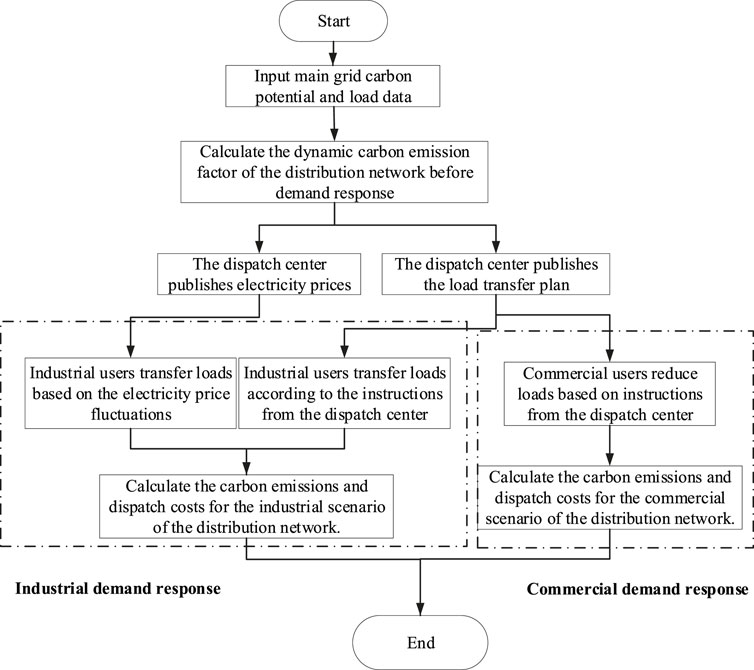
Figure 1. Demand response flowchart “or” demand response process diagram.

5 Case study

5.1 Basic data

For the modified IEEE 33-node system in the commercial load scenario, the locations of various photovoltaic (PV) units and energy storage are shown in Figure 2. In this study, three distributed PV units with a capacity of 400 kW each are installed at nodes 14, 19, and 28. Additionally, an energy storage system with a capacity of 400 kW/400 kWh is added at node 32.

Figure 2

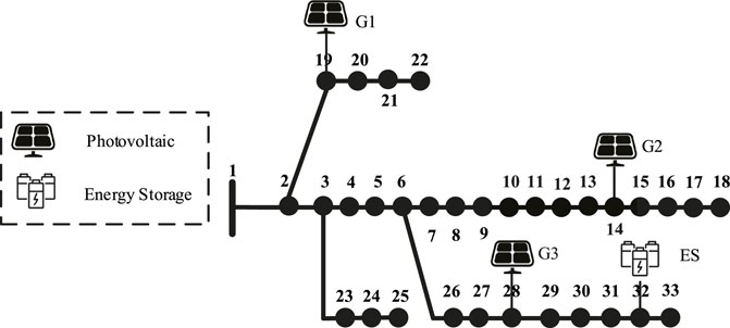
Figure 2. Schematic diagram of the modified IEEE 33-node system for the commercial load scenario.

Schematic diagram of the modified IEEE 33-node system for the industrial load scenario as shown in Figure 3. Distributed photovoltaic units with capacities of 1,000 kW are installed at nodes 6, 15, 20, and 28. Additionally, an energy storage device with a capacity of 1000 kW/1,000 kWh is added at node 32.

Figure 3

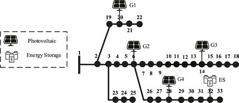
Figure 3. Schematic diagram of the modified IEEE 33-node system for the industrial load scenario.

The carbon potential of the main network has been predetermined, as referenced in [4], and its temporal distribution is illustrated in Figure 4.

Figure 4

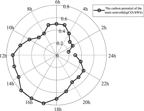
Figure 4. Distribution of main network carbon potential.

Distributed photovoltaic power generation is mainly influenced by the intensity of sunlight and is also affected by the temperature and humidity of the photovoltaic power generation equipment (Wu et al., 2019; Li et al., 2022b). In this paper, we mainly consider standalone photovoltaic power generation systems and do not consider the issue of power flow feedback. And energy storage and photovoltaic only provide output and do not participate in actual scheduling operations. The photovoltaic output is based on the power generated by a typical day during the summer solstice in a certain area of Jiangsu Province, sampled at 1-h intervals. The load data and photovoltaic output are shown in Figure 5.

Figure 5

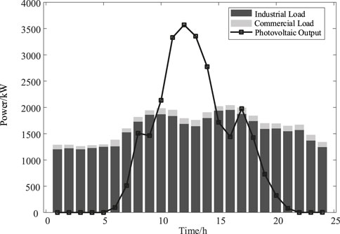
Figure 5. The data for photovoltaic output and load on the summer solstice day.

On the summer solstice day, the load exhibits a classic double-peak pattern. The commercial load output accounts for approximately 10% of the industrial load output. The photovoltaic (PV) output starts at 6 a.m., peaks around noon at 12 p.m., and concludes by 10 p.m. in the evening.

5.2 Analysis of optimization scheduling results for commercial load

The time period for reducing commercial loads is mainly concentrated from 12:00 to 19:00, while the load output remains unchanged in other time periods, as shown in Figure 6.

Figure 6

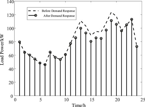
Figure 6. Comparison of commercial load demand response before and after.

Combined with Cplex solution, the results of traditional commercial load optimization scheduling are shown in Table 1. After traditional commercial load demand response on the summer solstice, it decreased by 4.71%, the scheduling cost decreased by 5.2%, carbon emissions decreased by 10.37%, and the compensation cost was 131.17 yuan.

Table 1

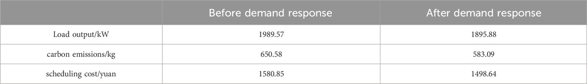
Table 1. Commercial load optimization scheduling results.

On the other hand, we also compared and analyzed the scheduling results using traditional carbon emission factors and improved carbon emission factors, as shown in Table 2. Due to the fact that scheduling costs do not involve carbon emission factors, whether traditional or improved carbon emission factors are used, scheduling costs remain unchanged; The improvement of the carbon emission factor takes into account the equivalent reduction in carbon emissions from photovoltaic waste, resulting in a decrease of 475.81 kg in carbon emissions compared to before the improvement.

Table 2

Table 2. Comparison of carbon emission factor scheduling results before and after commercial load improvement.

5.3 Analysis of industrial load optimization and scheduling results

Combining the distribution network and photovoltaic output data, the dynamic carbon emission factors of the distribution network before and after the improvement can be obtained, as shown in Figure 7. The positive half of the dynamic carbon emission factor on the Y-axis represents the overall carbon emission level of the distribution network, with values closer to zero indicating lower carbon emissions at that time. From 11 to 16 o’clock, when the photovoltaic output in the distribution network is high, the traditional carbon emission factor is zero, indicating the occurrence of curtailed photovoltaic power. However, it cannot reflect the difference in curtailed photovoltaic power at different times. The improved dynamic carbon emission factor shows negative values during curtailed periods, with higher absolute values indicating higher curtailed amounts, and values closer to zero indicating higher levels of renewable energy integration.

Figure 7

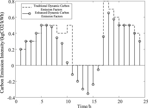
Figure 7. Comparison of dynamic carbon emission factors before and after improvement.

The paper divides the 24 h of a day into three electricity consumption periods: high carbon, medium carbon, and low carbon, based on the magnitude of carbon emissions. Each period consists of 8 h. The decision variable in this study is the time-of-use electricity price. The electricity price influences the amount of electricity consumed during different periods. Additionally, considering the variation in curtailed solar power during periods with negative carbon emission factors, the time-of-use electricity prices also differ accordingly. The time-of-use electricity prices after demand response are illustrated in Figure 8.

Figure 8

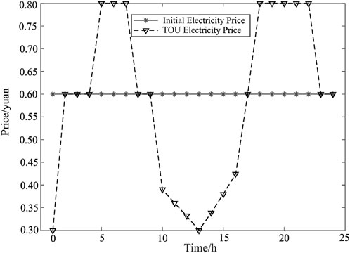
Figure 8. Time-of-use pricing for commercial load.

After demand response of industrial load, the distribution grid load is shifted from periods with higher carbon emission factors to those with lower carbon emission factors, as shown in Figure 9. The optimization results of demand response for industrial load are presented in Table 3. Compared to the situation before demand response, the carbon emissions have decreased by 1976.70 kg, and the curtailed solar energy rate has reduced by 4.73%. Additionally, the reduction in carbon emissions before and after demand response based on traditional carbon emission factors is 1250.38 kg. Considering the improved carbon emission factors after demand response, there is an increase of 36.7%. On the other hand, similar to the commercial load scenario, we also compared and analyzed the demand response scheduling results using traditional and improved carbon emission factors, as shown in Table 4. The scheduling cost remained unchanged, and the carbon emissions decreased by 1448.05 kg.

Figure 9

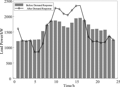
Figure 9. Comparison of industrial load before and after demand response.

Table 3

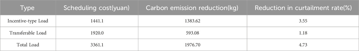
Table 3. The optimization results for industrial load.

Table 4

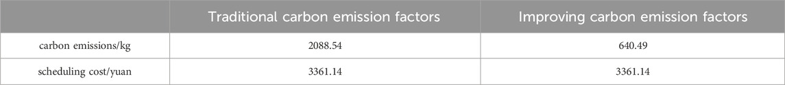
Table 4. Comparison of carbon emission factor scheduling results before and after industrial load improvement.

In addition, to verify the flexibility and transferability of the model, in a 96 node system, as long as the output of distributed power sources and energy storage is given, Still, like 33 nodes, demand response is achieved by adjusting electricity prices for different periods of carbon emission intensity, thereby optimizing the objective function of the entire distribution network (Yang et al., 2023). On the other hand, in the scenario examples involved in this article, due to the relatively simple 10 kV voltage level network, which does not involve many substations and distributed power sources, there is no need for a lot of nodes. Only 33 nodes are needed to simulate the distribution network in the real world and perform basic operation scheduling operations.

6 Conclusion

This paper proposes a low-carbon economic optimization scheduling model for the distribution network, considering an improved dynamic carbon emission factor to shift carbon emissions from the “source” side to the “load” side. Initially, based on the improved dynamic carbon emission factor, the method for calculating the carbon emissions of the distribution network is determined. Subsequently, for both commercial and industrial user scenarios, demand response models are established based on electricity prices and compensation fees, considering system scheduling and constraints. The distribution network is then optimized for scheduling from both economic and low-carbon perspectives. The proposed method is analyzed and validated through an improved IEEE 33-node system.

The results indicate that in the commercial user scenario, issuing load reduction commands during specified time periods from the dispatch center can effectively reduce the system’s scheduling costs and carbon emissions. In the industrial user scenario, incentives based on electricity prices and compensation fees guide users to shift loads from periods with higher carbon emissions to those with lower emissions. Additionally, during periods of high photovoltaic output, adjusting load consumption based on the amount of curtailed energy has increased the photovoltaic integration rate in the distribution network, reducing both carbon emissions and scheduling costs. It is hoped that in the future, this optimization method can be widely applied, and further research can explore coordinated strategies among generation, network, load, and storage to advance the development of the power industry (Pang et al., 2015).

Data availability statement

The raw data supporting the conclusion of this article will be made available by the authors, without undue reservation.

Author contributions

XR: Funding acquisition, Supervision, Writing–original draft. HG: Project administration, Writing–review and editing. XZ: Investigation, Writing–review and editing. JG: Data curation, Software, Writing–review and editing. LH: Methodology, Supervision, Writing–review and editing.

Funding

The author(s) declare that financial support was received for the research, authorship, and/or publication of this article. This work was supported by Science and Technology Project of State Grid Jiangsu Electric Power Company (“Assessment and Visualization of Low-carbon Technologies for Carbon Neutrality-oriented Distribution Network Framework,” Grant number: J2022118). The authors declare that this study received funding from Xuzhou Power Supply Company of State Grid Jiangsu Electric Power Supply Co Ltd. The funder was not involved in the study design, collection, analysis, interpretation of data, the writing of this article, or the decision to submit it for publication.

Conflict of interest

Authors XR, HG, and XZ were employed by Xuzhou Power Supply Company of State Grid Jiangsu Electric Power Supply Co Ltd.

The remaining authors declare that the research was conducted in the absence of any commercial or financial relationships that could be construed as a potential conflict of interest.

Publisher’s note

All claims expressed in this article are solely those of the authors and do not necessarily represent those of their affiliated organizations, or those of the publisher, the editors and the reviewers. Any product that may be evaluated in this article, or claim that may be made by its manufacturer, is not guaranteed or endorsed by the publisher.

References

Chen, H., Mao, W., and Zhang, R. (2021). Low carbon optimization scheduling of power system source load coordination based on carbon emission flow theory. Power Syst. Prot. Control 49 (10), 1–11. doi:10.19783/j.cnki.pspc.200932

CrossRef Full Text | Google Scholar

Chen, J., Wang, C., and Liu, C. (2023). Dynamic low-carbon dispatch method for power system based on improved carbon emission flow theory. China Electr. Power 56 (03), 162–172.

Google Scholar

Ge, J., Liu, Z., and Wang, C. B. (2023). Research on low-carbon optimization operation method of distribution system based on carbon emission flow. Power Grid Technol. 1-10. doi:10.13335/j.1000-3673.pst.2023.0602

CrossRef Full Text | Google Scholar

Ge, Y., Niu, C., Li, D., and Wang, C. (2022). “Low-carbon economic dispatch of distribution network with carbon capture power plant considering carbon trading,” in 2022 IEEE/IAS Industrial and Commercial Power System Asia (I&CPS Asia), Shanghai, China, July, 2022, 637–642. doi:10.1109/ICPSAsia55496.2022.9949729

CrossRef Full Text | Google Scholar

Han, G., Xiong, Li, and Xu, J. (2023). Environmental and economic scheduling of typical industrial load emission characteristics considering demand response. Automation Electr. Power Syst. 47 (08), 109–119.

Google Scholar

He, X., Liu, J., and Gao, H. (2023). Robust planning model for solar-energy storage distribution in industrial parks considering photovoltaic uncertainty and low-carbon demand response. Smart Power 51 (02), 69–76.

Google Scholar

Ibrahim, S., Laura, M., and Alparslan, M. Z. (2023). Voltage constraint-oriented management of low carbon technologies in a large-scale distribution network. J. Clean. Prod. 2023, 408.

Google Scholar

Kaile, Z., Lexin, C., Lulu, W., Xinhui, Lu, and Tao, D. (2020). A coordinated charging scheduling method for electric vehicles considering different charging demands. Energy 2020, 213. doi:10.1016/j.energy.2020.118882

CrossRef Full Text | Google Scholar

Kang, C., Chen, Q. X., and Xia, Q. (2009). “Research prospects of low-carbon power technology,” 33(02):1–7.

Google Scholar

Li, Y., Zhang, N., and Du, E. (2022a). Research on low-carbon demand response mechanism and benefit analysis of power system based on carbon emission flow. Chin. J. Electr. Eng. 42 (08), 2830–2842. doi:10.13334/j.0258-8013.pcsee.220308

CrossRef Full Text | Google Scholar

Li, Z., Guo, P., and Ma, N. (2022b). Reactive power optimization for distribution system with DG by particle swarm optimization algorithm integrating dual strategies. South. Power Syst. Technol. 16 (6), 14–22+81.

Google Scholar

Li, Z., Peng, X., Xu, Y., Zhong, F., Ouyang, S., and Xuan, K. (2023). A stackelberg game-based model of distribution network-distributed energy storage systems considering demand response. Mathematics 12 (1), 34. doi:10.3390/math12010034

CrossRef Full Text | Google Scholar

Lixia, C., and Yun, Z. (2023). Low carbon economic scheduling of residential distribution network based on multi-dimensional network integration. Energy Rep. 9 (S7), 438–448. doi:10.1016/j.egyr.2023.04.192

CrossRef Full Text | Google Scholar

Pang, S., Zhang, C., and Zhang, Di (2015). Optimization charging strategy for electric vehicles in residential communities based on adaptive mutation particle swarm optimization algorithm. Electr. Appl. 34 (20), 85–89.

Google Scholar

Qiang, L., Yan, J., and Changyu, D. (2023). Low-carbon optimization of distribution networks under the consideration of new energy integration. J. Phys. Conf. Ser. (1), 2659.

Google Scholar

Shao, Z., Zhao, Q., and Zhao, Y. (2021). Independent microgrid power supply coordination and configuration optimization. Power Grid Technol. 45 (10), 3935–3946. doi:10.13335/j.1000-3673.pst.2020.2028

CrossRef Full Text | Google Scholar

Shi, C., Zhu, Y., and Liu, Y. (2024). Low-carbon economic scheduling of wind power-inclusive power systems based on world model deep reinforcement learning. Grid Technol. 1-15. doi:10.13335/j.1000-3673.pst.2023.1899

CrossRef Full Text | Google Scholar

Song, Z., Hua, F., and Chen, X. (2023a). Distributed resource low-carbon scheduling strategy for distribution networks based on node carbon potential. High. Volt. Technol. 49 (06), 2320–2332. doi:10.13336/j.1003-6520.hve.20230216

CrossRef Full Text | Google Scholar

Song, Z., Hua, F., and Chen, X. (2023b). Low carbon scheduling strategy for distributed resources in distribution networks based on node carbon potential. High. Volt. Technol. 49 (06), 2320–2332. doi:10.13336/j.1003-6520.hve.20230216

CrossRef Full Text | Google Scholar

Wu, G., Wu, WANG, and Zhang, Y. (2019). Time decoupled dynamic extended reactive power optimization in incremental distribution network with photovoltaic-energy storage hybrid system. Power Syst. Prot. Control 47 (9), 173–179.

Google Scholar

Xiyun, Y., Lingzhuochao, M., Xintao, G., Ma, W., Fan, L., and Yang, Y. (2023). Low-carbon economic scheduling strategy for active distribution network considering carbon emissions trading and source-load side uncertainty. Electr. Power Syst. Res. 2023, 223. doi:10.2139/ssrn.4370986

CrossRef Full Text | Google Scholar

Xu, G., and Guo, Z. (2023). Resilience enhancement of distribution networks based on demand response under extreme scenarios. IET Renew. Power Gener. 18 (1), 48–59. doi:10.1049/rpg2.12895

CrossRef Full Text | Google Scholar

Xue, K., Chu, Y., and Zi, L. (2019). Low carbon economic optimization scheduling of integrated energy systems considering flexible loads. Renew. Energy 37 (08), 1206–1213. doi:10.13941/j.cnki.21-1469/tk.2019.08.016

CrossRef Full Text | Google Scholar

Yang, Mi, Zhou, J., and Lu, C. (2023). Multi-objective two-layer planning of distribution networks based on improved generative adversarial network and carbon footprint. Chin. J. Electr. Eng. 1-15.

Google Scholar

Zhang, H., Wang, R., and Liu, Y. (2023). Double layer low-carbon economic dispatch of power systems considering the coupling of source load carbon potential. Power Constr. 44 (12), 28–42.

Google Scholar

Zhou, T., and Kang, C. (2019). Research on low-carbon optimization operation method of distribution system based on carbon emission flow. Glob. Energy Internet 2 (03), 241–247. doi:10.19705/j.cnki.issn2096-5125.2019.03.005

CrossRef Full Text | Google Scholar

Zhou, T., Kang, C., and Xu, Q. (2012). Theoretical exploration of carbon emission flow analysis in power systems. Automation Electr. Power Syst. 36 (07), 38–43+85.

Google Scholar

Zhou, N., Fan, W., and Liu, N. (2016). Multi-target capacity optimization configuration of photovoltaic microgrid energy storage system based on demand response. Power Grid Technol., 1–10. doi:10.13335/j.1000-3673.pst.2023.0602

CrossRef Full Text | Google Scholar