 Fanny Kristianti1*
 Franziska Gerber1,2
 Sergi Gonzàlez-Herrero2
 Jérôme Dujardin1,2
 Hendrik Huwald1,2Sebastian W. Hoch3
 Michael Lehning1,2
- 1Environmental Engineering Institute, Laboratory of Cryospheric Sciences, Ecole Polytechnique Fédérale de Lausanne (EPFL) Valais/Wallis, Sion, Switzerland
- 2WSL Institute for Snow and Avalanche Research SLF, Davos, Switzerland
- 3Department of Atmospheric Sciences, University of Utah, Salt Lake City, UT, United States
Wind energy is one of the potential options to fill the gap in renewable energy production in Switzerland during the winter season when the energy demand exceeds local production capacities. With likely further rising energy consumption in the future, the winter energy deficit may further increase. However, a reliable assessment of wind energy potential in complex terrain remains challenging. To obtain such information, numerical simulations are performed using a combination of the “Consortium for Small-scale Modeling” and “Weather Research and Forecasting” (COSMO-WRF) models initialized and driven by COSMO-1E model, which allows us to simulate the influence of topography at a horizontal resolution of 300 m. Two LiDAR measurement campaigns were conducted in the regions of Lukmanier Pass and Les Diablerets, Switzerland. Observational LiDAR data and measurements from nearby wind sensor networks are used to validate the COSMO-WRF simulations. The simulations show an improved representation of wind speed and direction near the ground compared to COSMO-1E. However, with increasing height and less effect of the terrain, COSMO-WRF tends to overestimate the wind speeds, following the bias that is already present in COSMO-1E. We investigate two characteristic mountain–terrain flow features, namely waves and Foehn. The effect of mountain-induced waves of the flow is investigated through an event that occurred in the area of Diablerets. One-year analysis for the frequency of conditions that are favorable for mountain wave formation is estimated. The Foehn impact on wind was observed in the Lukmanier domain. We attempt quantification of the probability of occurrence using the Foehnix model. The result shows a high probability of Foehn occurrence during the winter and early spring seasons. Our study highlights the importance of incorporating complex terrain-related meteorological events into the wind energy assessment. Furthermore, for an accurate assessment of wind speed in complex terrain, our study suggests the necessity to have a better representation of the topography compared to COSMO-1E.
1 Introduction
Switzerland has stated the objective to entirely transition to renewable energy resources as formulated in the Energy Strategy 2050 (Swiss Federal Office of Energy, 2023b). It is therefore crucial to explore renewable energy options, to reduce and replace the use of unsustainable fossil fuels and thus reduce greenhouse gas emissions (Sims, 2004; Olabi and Abdelkareem, 2022). Currently, the largest part of Switzerland’s renewable energy production is based on hydropower (Swiss Federal Office of Energy, 2023a). However, the mismatch of over-production during summer and a demand exceeding production during winter constitutes a significant challenge, i.e., seasonal peaks of production and demand are not aligned. During summer, hydro-power production increases due to the seasonal snow melt and precipitation dynamics (Bavay et al., 2009), while in winter the energy demand increases (Dujardin et al., 2017). Dujardin et al. (2021) suggests that adding wind as a renewable energy resource could be part of the solution to alleviate this energy mismatch. A general increase in mean wintertime wind speed in North and Central Europe has been reported, fueling the motivation to explore the wind as potential energy resource (Archer and Jacobson, 2013; Graabak and Korpås, 2016; Clark et al., 2017; Grams et al., 2017).
The Alps cover two-thirds of Switzerland’s area (Federal Office of Topography, 2023). These complex terrain characteristics add to the difficulty of assessing the wind energy potential of the country (Alfredsson and Segalini, 2017; Lange et al., 2017; Mann et al., 2017). The characteristic spatial and temporal patterns of the wind vary substantially according to the specific local topography of the complex terrain. This makes it difficult to accurately observe and quantify near-surface flow using standard measurement techniques and instrumentation (Kruyt et al., 2018), in particular due to sparse spatial distribution of instruments. Most of the wind measurements are taken near the surface at 10 m above ground (MeteoSwiss, 2022; WSL SLF, 2022), while most of the operational wind turbines feature a hub height of 100 m. A logarithmic wind profile is often utilized to extrapolate the wind speed measured near the ground to the turbine hub height. However, the vertical wind profile in complex terrain generally does not follow a logarithmic shape (Dar et al., 2019; Elgendi et al., 2023). Despite the additional problems and challenges, it has been found that terrain complexity can also provide benefits to the local wind power potential (Clifton et al., 2014). If this mechanism is well understood, the interplay between wind and complex terrain could be an untapped potential for wind energy resources. To estimate local wind speed in complex terrain at typical turbine hub heights where measurements are unavailable, several simulation techniques, such as computational fluid dynamics (CFD) (Dhunny et al., 2017; Tabas et al., 2019) and numerical weather models (NWP) Kruyt (2019), have been used while available measurements serve for validating the accuracy of the simulations.
Simulating airflow over complex terrain requires the ability of a model to combine the synoptic flow field and regional scale topography (Lehner and Rotach, 2018). However, the high computational demand of CFD and NWP models and limited computer resources make it difficult to simulate with a fine grid and sufficient domain size for a sufficiently long period to represent the synoptic scale processes. On the other hand, running the model in a too-coarse resolution often results in incorrect, unrealistic representation of the local topography, making it inadequate for resolving the complex terrain processes (Toumelin et al., 2023). The accurate representation is essential for reliable wind energy assessment in complex terrain where the spatial and temporal variability of wind speed is high (Pickering et al., 2020; Clifton et al., 2022; Dujardin and Lehning, 2022). Currently, assessments of large-scale wind resources are often based on reanalyses with a typically very coarse horizontal resolution of 50–100 km and a coarse time step of 1–3 h (Archer and Jacobson, 2005; Archer and Jacobson, 2013; Tobin et al., 2015; Grams et al., 2017). In such a framework, significant wind energy potential in complex terrain likely remains undiscovered due to insufficient spatial resolution for capturing local topographic effects.
In this paper, we propose to simulate wind in complex terrain at a spatial resolution of 300 m, i.e., a resolution within the so-called gray zone (Chow et al., 2019) (also referred to as “terra incognita” in the context of turbulence modeling (Wyngaard, 2004)). The gray zone is a range of resolutions for which certain physical processes start to be explicitly resolved (approximately 100 m to 1 km, Kealy et al. (2019)). When modeling turbulence, it is defined when the turbulence length scale is comparable to the filter length scale (Wyngaard, 2004). In the context of complex terrain, the gray zone challenges include the correct representation of topography, turbulence, and convective processes (Chow et al., 2019). For the scale of the Swiss Alps complex terrain, running simulations at gray zone resolution is cheaper in computational resources compared to classical micro-scale simulations. Another benefit of simulations in the gray zone is to have more insight into the interplay between the meso-scale motion and the smaller-scale motion that occurs at the higher resolution scale because it allows for larger domains to be covered compared to microscale simulations. The representation of the interplay of flow at the two different scales is crucial for gaining accurate information on the wind energy potential in complex terrain (Koletsis et al., 2009; Koletsis et al., 2010).
A previous study by Gerber et al. (2018) implemented the Weather Research and Forecasting (WRF) model (Skamarock et al., 2008), initialized by a 2.2 km resolution Consortium for Small-scale Modeling (COSMO) analysis. This model, hereafter called COSMO-WRF, was used to study wind and terrain-controlled distribution of snow in the complex terrain of Dischma Valley near Davos, Switzerland. The results of the simulation were validated and discussed against operational weather radar measurements acquired at the nearby Weissfluh summit provided by the Federal Office of Meteorology and Climatology (Meteoswiss). Kruyt (2019) have also used COSMO-WRF simulations to investigate the wind speed at a 450 m horizontal grid resolution in the Swiss Alps. That resolution resulted in a significant improvement of the representation of wind speed at the hub height of wind turbines and in the prediction of resulting power production, compared to the results of simulations using COSMO-1 alone, which has a spatial resolution of 0.01°. This improvement is attributed to the better terrain representation in the model. Results from these studies motivate us to further explore the utilization of numerical weather models for the study of wind speed in complex terrain areas. We combine WRF and an ensemble of 11 forecasts with a spatial resolution of 1.1 km called COSMO-1E (Federal Office of Meteorology and Climatology MeteoSwiss, 2023a) to study the flow in complex terrain.
Understanding the impact of typical wind features in complex terrain on potential wind energy production is crucial. Examples of complex terrain phenomenon that affect wind power production are mountain waves (Draxl et al., 2021; Xia et al., 2021) and Foehn wind (Pickering et al., 2020). Mountain waves tend to occur when a stably stratified air mass ascends a mountain barrier and triggers buoyancy perturbations when it descends on the lee side of the barrier. The wave oscillation on the lee side can result in a disturbance of the airflow, which can be propagated downward to a level of 90 m above ground, as shown in the METCRAX II field experiment (Lehner et al., 2016). It has also been reported that mountain wave fluctuations can change the total power output of a wind farm in the region of the Columbia River (United States) up to 11% (Draxl et al., 2021). Foehn wind, on the other hand, is a strong, warm, and dry down-slope wind (Chow et al., 2013). A statistical mixture model named Foehnix (Plavcan et al., 2014) can be used to separate the Foehn and non-Foehn events. This model was tested in the Wipp Valley, Austria, using wind data of a station situated on the crest (Sattelberg station, 11.47889° E/47.01083° N, 2107 m a.s.l.) and a station in the valley (Ellbögen station, 11.42889° E/47.18694° N, 1,080 m a.s.l.). The complex terrain phenomenon mentioned above have typically not been included in the wind energy assessment process. Understanding these events can lead to a better selection for wind turbine infrastructure and to a more accurate forecast of energy production. Therefore in this paper, we study the effect of mountain waves and Foehn on the wind in the Alpine area, as two examples of complex terrain effects.
Data and results from a measurement campaign in the Swiss Alps using a Light Detection and Ranging (LiDAR) instrument, combined with simulation results from COSMO-WRF are used to investigate the impact of complex terrain phenomenon on wind speed. Wind LiDAR instruments were used in previous experiments to measure mountain waves (Lehner et al., 2016; Udina et al., 2020) and Foehn events (Beffrey et al., 2006). A filtering technique to derive wind speed in complex terrain using LiDAR measurements is provided in Kristianti et al. (2023). This technique was tested for data obtained at the Diablerets and Lukmanier areas, both Swiss Alps (Figure 1), during the winter season of 2020/21.
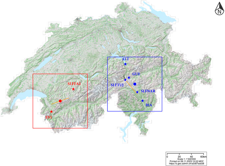
Figure 1. Simulation domains of Diablerets (red box) and Lukmanier (blue box). The LiDAR locations in Diablerets and Lukmanier are shown by red and blue dots, respectively. Star symbols represent the SMN and IMIS wind measurement stations. The orange line inside the Diablerets domain represents the vertical cross-section shown in Figure 10. The black and orange line inside the Lukmanier domain represents the vertical cross-section shown in Figure 14. Map source: (Federal Office of Topography, 2023).
This paper aims to propose a method for studying the spatial variability of wind speed in complex terrain and quantifying the effect of complex terrain phenomenon on wind speed. We propose the use of COSMO-WRF simulations in the so-called gray zone of spatial resolution to obtain information on wind interplay between the synoptic and local scales. Two complex terrain phenomenon, namely waves and Foehn, are analyzed to study the impact on wind speed in Swiss Alps area. The focus of the study is on the wind assessment process, for which many aspects also need to be considered (i.e. potential of social impact, etc), however, we limit the scope of the study to wind potential only. Section 2 describes the methods used for the assessment process. Details about the wind measurement network and the LiDAR measurement campaign are described in Sections 2.1.1, 2.1.2, respectively. We also provide a short description of the models used in this study, namely COSMO-1E (Section 2.2.1), COSMO-WRF (Section 2.2.2), and Foehnix (Section 2.2.3). The validation of wind simulations in the gray zone resolution is discussed in Section 3.1. The analysis of the complex terrain wind features is presented in Sections 3.2, 3.3 for mountain waves and Foehn, respectively. The main findings and conclusion are summarized in Section 4.
2 Data and methods
2.1 Measurements
2.1.1 Wind measurement network
Data from two wind measurement networks are used to validate the COSMO-WRF simulation: (a) the Inter-Cantonal Measurement and Information System, IMIS (WSL SLF, 2022), and (b) the Meteo Swiss SwissMetNet, SMN (MeteoSwiss, 2022). By 2021, the IMIS network counts 186 measuring stations which are scattered over the Swiss Alps. The IMIS stations are situated at high-elevation locations to provide data for operational avalanche forecasts and warnings. IMIS wind speed data are measured by R.M.Young wind sensors (model 05103) at approximately 7.5 m a.g.l. (Lehning et al., 2000). SMN stations are distributed at middle and low altitudes of Switzerland. SMN measures wind speed using Lambrecht L14512 cup anemometers and Thies 2D ultrasonic anemometers at 10 m a.g.l. (Federal Office of Meteorology and Climatology MeteoSwiss, 2023b).
The stations used for validation of the COSMO-WRF simulation and as input for the Foehnix model are shown in Figure 1 (star symbols) and station details are given in Table 1. Stations Nara/Motto Crostel (SLFNAR) and Tujetsch/Crispalt (SLFTUJ) are used for COSMO-WRF validation of the Lukmanier domain and stations Evionnaz (EVI) and Färmel/Färmelberg (SLFFA2) are used for COSMO-WRF validation of the Diablerets domain. SLFNAR is located on the peak of Motto Crostel, in the middle of Valle Leventina and Valle di Blenio, Canton Ticino, Switzerland. SLFTUJ is located on the Crispalt ridgeline, on the northwest side of Oberalpass, Canton Glarus, Switzerland. EVI is located in Evionnaz city on the west side of the Rhone Valley in Canton Valais and SLFANV is located in Färmelberg, Canton Bern. The stations Altdorf (ALT), Biasca (BIA), and Gütsch (GUE) are used as input data for the Foehnix model. Both ALT and BIA stations are used as valley stations for the Foehnix model. ALT is used to represent the southerly Foehn. BIA is used to represent the northerly Foehn. GUE is used as crest station input of the Foehnix model for both northerly and southerly Foehn.
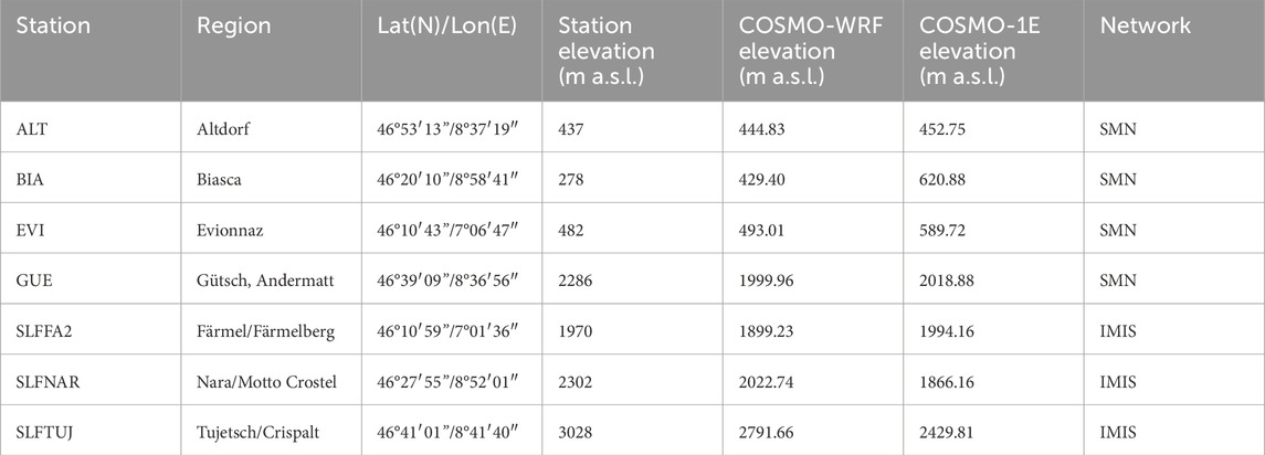
Table 1. Details of the SMN and IMIS wind measurement stations.
2.1.2 LiDAR measurements
Two measurement campaigns were conducted deploying a Halo Photonics Streamline XR Scanning Doppler wind LiDAR. The first field campaign was conducted on the west slope of Piz Scopi, Lukmanier, and the second campaign was conducted at Cabane station, Diablerets (dots in Figure 1). The Lukmanier and Diablerets campaigns were conducted from 20/10/2020 to 16/12/2020, and from 20/02/2021 to 02/05/2021, respectively. The coordinates of the LiDAR location were 46.58409° N, 8.81890° E (blue dot, Figure 1) at 2519 m a.s.l. at Lukmanier, and 46.33995° N, 7.21491° E (red dot, Figure 1) at 2523 m a.s.l. at Diablerets. The LiDAR configuration was the same for both campaigns except for the elevation angle of 45° at Lukmanier and 70° at Diablerets. The gate overlapping mode was used to collect LiDAR data, with a range gate length of 30 m. This resulted in radial velocity retrieval from 30 m gates with a 3-m spacing. Under ideal conditions, the use of this setting enables us to observe wind velocity up to a radial distance of 2.1 km. We used 6-point and 12-point step-stare Plan Position Indicator (PPI) scans at an elevation angle of 45° and 70° for Lukmanier and Diablerets sites, respectively. The scan sequence was repeated at 5- and 10-min intervals for the Lukmanier and Diablerets sites, respectively. Post-processing from the radial velocity to the u, v, w wind speed components followed the procedure described in Kristianti et al. (2023).
2.2 Models
2.2.1 COSMO-1E
COSMO-1E is a numerical weather forecasting model run over Switzerland at a horizontal resolution of 1.1 km (Federal Office of Meteorology and Climatology MeteoSwiss, 2023a). COSMO-1E includes an ensemble of 11 forecasts computed eight times per day. From a single forecast, several iterations are produced to predict the probability of weather events. Therefore, the reliability of the forecast is improved and so is the quality of short to medium-range forecasts for extreme or highly localized weather, compared to the deterministic forecast (Schraff et al., 2016).
2.2.2 COSMO-WRF
Numerical modeling is used to investigate the spatial variations of wind speed in complex terrain and its effect on the wind at typical turbine hub heights of 100 m above ground level. We use the Weather Research and Forecasting (WRF) model, Version 4.4.5 (Skamarock et al., 2021) initialized and forced with COSMO-1E (Federal Office of Meteorology and Climatology MeteoSwiss, 2023a) data provided by Meteoswiss (COSMO-WRF, hereafter). COSMO-WRF is used to simulate representative cases of flow events over the complex terrain at the Diablerets and Lukmanier sites based on observational LiDAR data. The topography input is based on the Advanced Spaceborne Thermal Emission and Reflection Radiometer (ASTER) global digital elevation model (DEM) v003 (NASA/METI/AIST/Japan Space systems and U.S./Japan ASTER Science Team, 2019) and the land use is taken from the Coordination of Information on the Environment (CORINE) dataset (European Environmental Agency, 2006) as provided by Gerber and Lehning (2021). More technical details about COSMO-WRF can be found in (Gerber and Sharma, 2018).
Owing to the steep slopes in the selected complex terrain domains, which may lead to numerical instabilities in the simulations, a pre-processing of the topographic data is needed. Pre-processing of WRF is performed by using the WRF Pre-processing System (WPS) Version 4.4 (Skamarock et al., 2021). We use three cycles of the 1-2-1 smoothing algorithm to reduce steep slopes over 45° (Gerber and Sharma, 2018). After the smoothing process, the maximum slope angle in the simulation domain is 46.1° and 43.6° for the Lukmanier and Diablerets sites, respectively. The simulation domains are set to 90 × 90 km, with the LiDAR position located at the center (Figure 1). A single domain with no nesting is used for the simulations, following the gray zone recommendation of Chow et al. (2019). The horizontal grid resolution is 300 m resulting in a domain composed of 301 × 301 grid points.
The model applies eta-level coordinates with 60 vertical levels. The simulation is run with a time step of 0.5 s. The barometric pressure at the top of the domain is set to 15′000 Pa. The planetary boundary layer uses the Shin-Hong Scale scheme (Shin and Hong, 2015). The Morrison 2-moment scheme is selected (Morrison et al., 2009) to parameterize the cloud microphysics. Longwave and shortwave radiation use the rrtmg parameterization (Mlawer et al., 1997). For the surface layer a Monin-Obukhov Similarity scheme is implemented (Dyer and Hicks, 1970; Paulson, 1970; Webb, 1970; Zhang and Anthes, 1982; Beljaars, 1995). Land surface processes are parameterized by the Noah-MP scheme (Niu et al., 2011; Yang et al., 2011). No cumulus option is used when running WRF. The w-Rayleigh damping option (Klemp et al., 2008) is activated in WRF. The namelist used to prescribe the simulation can be found on (Kristianti et al., 2024). At the grid cells where the wind measurement stations and LiDAR are located, model output is saved at every time step using the tslist options of the WRF model.
Two representative flow situations are simulated for each field site, resulting in four simulation cases (two cases for Lukmanier and two cases for Diablerets). For the Lukmanier site, observations of 23/10/2020 and 09/12/2020 are used to represent the southerly and northerly flow regimes, the two principal wind directions during the campaign duration. For Diablerets, observations of 27/02/2021 and 11/03/2021 are used to represent the easterly and southwesterly flow regimes, the two principal wind directions during the campaign. A more detailed wind direction analysis can be found in Kristianti et al. (2023). Details of the simulations are summarized in Table 2.
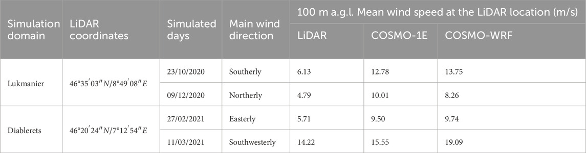
Table 2. Simulation details.
2.2.3 Foehnix
Foehn events are investigated and validated using a statistical mixture model named Foehnix (Plavcan et al., 2014). The model can distinguish between Foehn and no Foehn wind using wind speed, wind direction, relative humidity, and temperature differences as indicators. First, a wind direction filter is applied. Then, the temperature difference between the two stations is selected as the dominant variable, while wind speed and relative humidity are used as concomitant variables. The mixture model uses the wind speed distribution and divides it into downslope wind and Foehn. The Foehn phenomenon has a strong seasonal cycle, therefore to capture this cycle, a minimum data set comprising at least 1 year is required as model input.
2.3 Power curve of wind turbine
The wind turbine power curve can be used as a tool to estimate the power extractions from the incoming wind speed. A typical wind turbine power curve consists of four regions of wind speed (Figure 2). The first region represents the area where wind speed is less than the minimum wind speed for power production (vcut_in), therefore it does not produce any power. The second region represents the area between the vcut_in and the rated wind speed (vrated). In this region, the power rises rapidly until the wind speed reaches the vrated. The third region produces a constant power where the wind speed is between the vrated and the maximum operational wind speed (vcut_off). If the wind speed goes higher than the (vcut_off), the wind turbine does not operate to protect its components from possible damage due to high wind. The wind speed above the (vcut_off) is represented in the fourth region, which produces no power, similar to the first region.

Figure 2. Schematic diagram of typical power curve of wind turbine.
3 Results and discussion
3.1 Validation of wind simulation
This section compares the wind simulation results from COSMO-WRF to the LiDAR and wind station measurements at the two field sites. Three aspects of wind (direction, vertical profiles, and time series of wind speed) are utilized for this purpose. In addition, a comparison with COSMO-1E data is provided. The comparison with wind station data represents the conditions near the ground level and the comparison with LiDAR data represents the conditions at a higher elevation level.
The comparison of the observed daily averaged LiDAR wind speed and wind direction profiles, the COSMO-1E, and the COSMO-WRF simulations for four different periods is presented in Figures 3A-H. The wind speed profiles in the top row show that both COSMO-1E and COSMO-WRF overestimate the wind speed compared to the LiDAR measurements, especially at low elevations (Figures 3A, C). A relatively good agreement of the wind direction profile between measurement, COSMO-1E, and COSMO-WRF can be seen for the profiles with little change of wind direction with height (Figures 3E, H). However, the marked wind direction change with height (veering or backing) (Figures 3F, G), was neither captured in COSMO-1E nor COSMO-WRF. The slightly improved representation of the COSMO-WRF wind direction profile especially near the ground compared to COSMO-1E (Figure 3F), may be explained by the better terrain representation in COSMO-WRF compared to COSMO-1E. However, with increasing height and lower influence of the terrain, the wind direction follows COSMO-1E as this is used as forcing. The wind direction change from 200° (southerly) to 100° (easterly) in the lowest 300 m above ground level (Figure 3G) is also not represented by both models. The wind direction profile from COSMO-1E and COSMO-WRF is rather constant with height (approximately 100° and agrees well with observations higher than 300 m a.g.l.
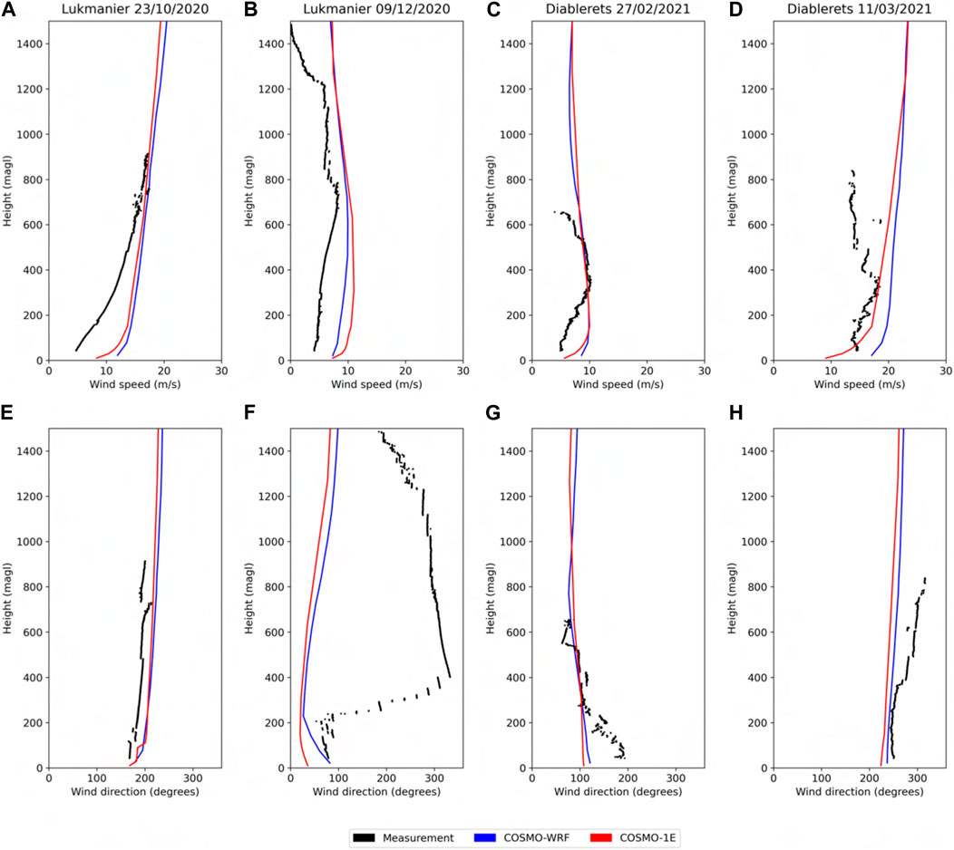
Figure 3. Daily average wind speed (top) and wind direction (bottom) profile at the field sites measured by the LiDAR (black), and simulated by COSMO-WRF (blue), and COSMO-1E (red) during 23/10/2020 (A,E) and 09/12/2020 (B,F) in the Lukmanier domain, and 27/02/2021 (C,G) and 11/03/2021 (D,H) in the Diablerets domain.
Overall, COSMO-1E and COSMO-WRF show wind speed overestimation in all wind speed profiles and some disagreements in wind direction, especially for profiles with veering winds. This disagreement illustrates the complexity of the wind in mountain regions and the difficulty of simulating it. The overestimation of wind speed by COSMO-WRF can be explained by the overestimated input data from COSMO-1E. Table 2 presents the 100 m a.g.l. mean wind speed at the LiDAR location in COSMO-1E and COSMO-WRF, representing a wind turbine hub height. Compared to the LiDAR measurements, the simulated wind speed is overestimated by approximately 5 m/s by both models.
Further analysis compares the time series of wind speed and the wind roses from COSMO-WRF and COSMO-1E to wind measurement stations. Figures 4, 5 show wind roses and time series of wind speed at wind measurement stations situated in the Lukmanier and Diablerets domains, respectively. Details of these measurement stations used for validation can be seen in Table 1. For the case study of 23/10/2020 (Figures 4A, C), the wind roses from COSMO-1E and COSMO-WRF at SLFNAR and SLFTUJ show more distributed directions compared to the observations, which are mainly clustered around the southerly (SLFNAR) and southwesterly (SLFTUJ) sectors. The observed difference in wind direction is explained by the COSMO-1E wind direction input data, while COSMO-WRF shows a slight deviation from its initial direction in COSMO-1E. For the case study of 09/12/2020 (Figures 4E, G), on the other hand, the wind rose shows better agreement between the measurements, COSMO-1E, and COSMO-WRF.
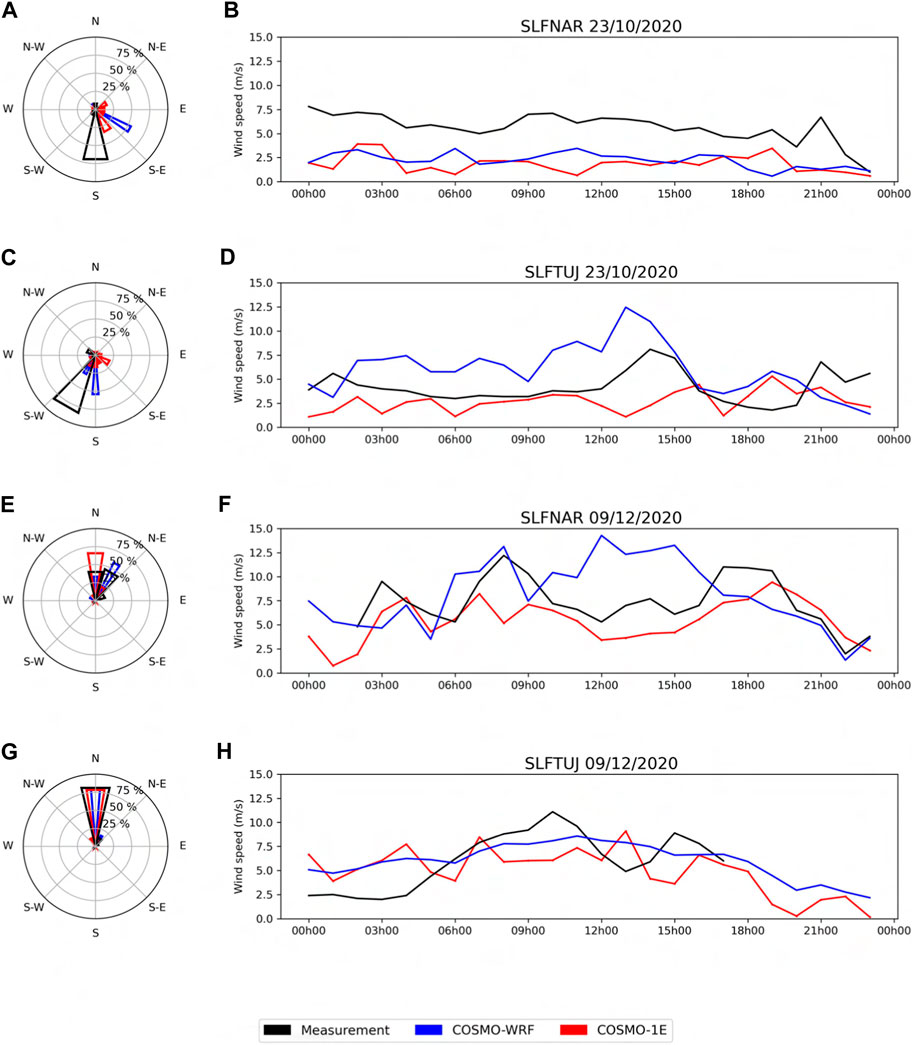
Figure 4. Windrose (left) and wind speed time series (right) from the Lukmanier simulation domain at SLFNAR (A,B,E,F) and SLFTUJ (C,D,G,H) stations on 23/10/2020 (A,B,C,D) and 09/12/2020 (E,F,G,H). The black color shows the result of the wind measurement station, the blue color shows the COSMO-WRF result and the red color shows the COSMO-1E. On 09/12/2020 (H), some observational data is missing during the night for the SLFTUJ station.
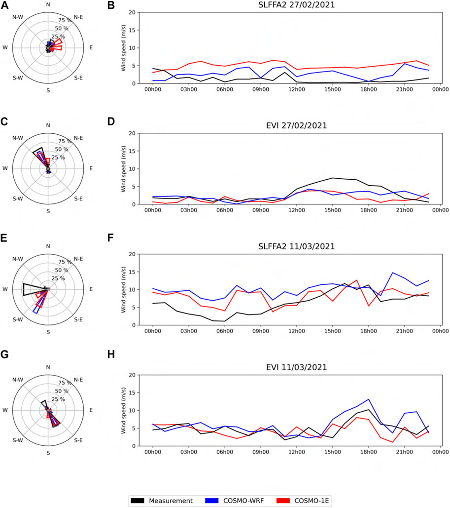
Figure 5. Windrose (left) and wind speed time series (right) from the Diablerets simulation domain at EVI (A,B,E,F) and SLFFA2 (C,D,G,H) stations on 27/02/2021 (A,B,C,D) and 11/03/2021 (E,F,G,H). The black color shows the result of the wind measurement station, the blue color shows the COSMO-WRF result and the red color shows the COSMO-1E.
Figures 4B, D, F, H show the wind speed time series at the SLFNAR and SLFTUJ station, respectively. The time series of wind speed shows an underestimation by COSMO-1E and COSMO-WRF compared to the measurements, except in the COSMO-WRF case of SLFTUJ on the 23/10/2020 and SLFNAR on the 09/12/2020. This contradicts the comparison between LiDAR and simulation profiles, where COSMO-1E and COSMO-WRF overestimate the wind speed (Figure 3). This might be the result of a lower elevation represented in COSMO-1E and COSMO-WRF, compared to the real elevation of the SLFNAR and SLFTUJ stations (Table 1). During the smoothing process in WPS, the steepness of the slope in COSMO-WRF is reduced. After smoothing, to reach a maximum steepness of approximately 45°, topographic peaks get “shaved” and valleys are “filled.” The elevation difference is more significant for the near ground level wind speed, where the comparison with wind measurement stations is performed. At higher elevations, as we can see from the comparison with LiDAR, COSMO-WRF tends to be closer to COSMO-1E as the terrain influence diminishes. A slight improvement in the near-ground wind speed comparison from COSMO-WRF (right column, Figure 4) can be the result of a smaller elevation difference between COSMO-WRF and the stations compared to COSMO-1E and the stations (Table 1) since with 300 m horizontal grid resolution COSMO-WRF has a better terrain representation than the 1 km of COSMO-1E.
Figure 5 shows the comparison of wind direction and wind speed time series for the Diablerets domain. For 27/02/2021 at the SLFFA2 station (Figure 5A), observed winds are from all directions, while COSMO-WRF, and COSMO-1E show dominant NE-E directions. For the case study of 11/03/2021 at SLFFA2 station (Figure 5E), measurements show a significant difference in wind direction compared to the models, which could be due to the local terrain sheltering of the station still insufficiently resolved. The time series of wind speed (Figures 5B, F), show a slight overestimation by COSMO-1E and COSMO-WRF at the SLFFA2 location which may again be due to an overestimation of the SLFFA2 station elevation in COSMO-1E. This would result in an overestimation of wind speed from COSMO-1E compared to the measurement. On 27/02/2021 at EVI station (Figure 5C), the wind directions from models and measurements are well aligned. On 11/03/2021 at EVI station (Figure 5G), the modeled wind direction (SE) is well aligned with part of the measured wind, however, the other part is opposite to the modeled wind. At the EVI station, the measured and modeled wind speed time series show a good agreement (Figures 5D, H). For wind speed near ground level, COSMO-WRF seems to perform well, if the model terrain elevation in COSMO-WRF is similar to the real terrain elevation. This explanation is consistent with a better agreement of both elevation and near-ground time series of wind speed at the SLFFA2 and EVI stations, compared to the SLFNAR and SLFTUJ stations. At higher elevations of the atmosphere, however, the influence of the input and boundary conditions from COSMO-1 in the COSMO-WRF model becomes stronger and might result in overestimation.
In conclusion, COSMO-WRF shows improved simulation results near the ground compared to COSMO-1E, as a result of the better terrain representation in COSMO-WRF. However, model performance is limited by the input data used (COSMO-1E), which tends to overestimate the wind speed at the height, where the wind turbines are located (cf. Table 2). Therefore, existing biases in the forcing data aloft cannot be completely rectified with improved surface representation. The COSMO-WRF simulations are improving surface representation but remain limited due to the (still) coarse horizontal resolution of 300 m and the maximum allowed slope angle of approximately 45°. These two limitations bear the risk of compromising the terrain’s full influence. As the simplification of the terrain leads to an overestimation or underestimation of wind speed depending on the location, it is important to use multiple sites for a robust and representative comparison between models and measurements. The further use of the COSMO-WRF model in this study is to study and quantify the effect of complex terrain on wind power potential, thus the model needs to capture the event mechanism. This will contribute to the main goal of our study, namely for a better understanding of the possible mechanism of Foehn and mountain waves that influence wind variability in complex terrain.
3.2 Influence of mountain waves on wind speed at turbine hub height
This section aims to investigate how events of mountain waves influence the wind at the hub height of a potential turbine at the Diablerets site and to quantify the conditions favoring the generation of mountain waves. By utilizing satellite images, the observed mountain wave event is validated and analyzed using COSMO-WRF simulations. Afterward, we describe the effect of mountain waves at turbine height levels and underline the importance of including this aspect in wind energy assessment in complex terrain.
For finding a mountain wave, the high wind speed period measured at Diablerets on 11/03/2021 is selected (Figure 6, blue dots). The area within the white box in Figure 7A is selected to check the corrected reflectance from Moderate Resolution Imaging Spectro-Radiometer (MODIS) satellite images on 11 and 12 March 2021 (Figures 7B, C). On 12/03/2023 (Figure 7C), we see cloud bands, perpendicular to the wind over the Alps, as seen from the LiDAR’s wind rose (Figure 9A). This cloud pattern is associated with mountain waves that often occur downwind of a mountain when the atmosphere is stably stratified, especially during the winter season. A similar pattern can also be seen in the blue-circled area on 11/03/2021 and 12/03/2021, suggesting the event lasted for 2 days. Due to the limited availability of LiDAR data on 12/03/2021, only data from 11/03/2021 are analyzed. Over Switzerland, COSMO-1E at approximately averaged 2,400 m a.g.l. of terrain following coordinates show a pattern of alternating positive and negative vertical wind velocities (Figure 8). The horizontal wind direction is consistent with the LiDAR’s wind rose and the cloud pattern shown in the satellite images. The simulated wave pattern is strongest in the southwestern Alpine region (tallest mountains) and weakest over the (Rhone River) valley. However, the alternating vertical velocity pattern covers most of Switzerland, apart from the Ticino region in the South. This shows the wide impact area of the wave event and the importance of understanding the event to accurately assess its influence.
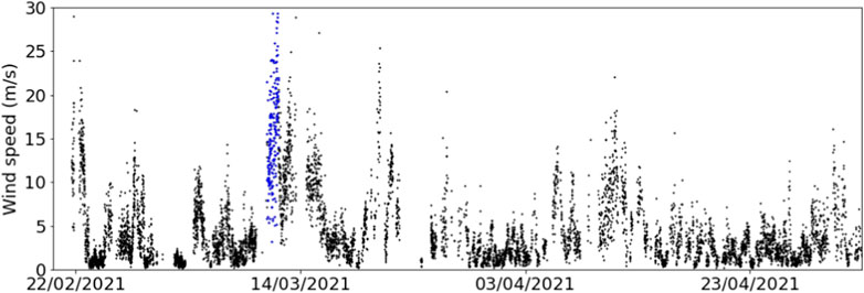
Figure 6. LiDAR wind speed measurements at Diablerets from 20/02/2021 to 02/05/2021 (black dots) and the simulation period on 11/03/2021 (blue dots) at 100 m a.g.l.
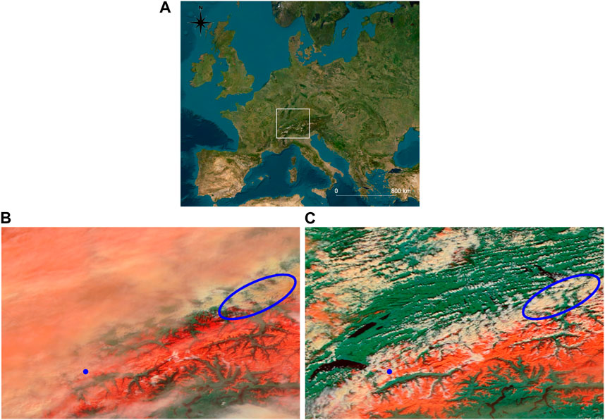
Figure 7. (A) Selected area (white rectangle) of the MODIS satellite images [map source (ESRI, 2023)]. EOSDIS satellite image [source: NASA EARTHDATA (2023)] on (B) 11/03/2021 and (C) 12/03/2021 of the region indicated in (A) at 60-m resolution. Snow and ice on the surface are shown in red color. Green and white represent land and clouds, respectively. The blue dot indicates the Diablerets site.
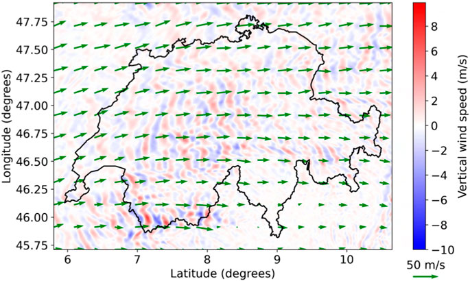
Figure 8. Vertical velocity from the terrain following coordinate of COSMO-1E with average height of 2,400 m a.g.l. on 11/03/2021, 12h00. Green arrows represent the horizontal wind speed and direction. The red and blue colors represent upward and downward vertical velocity, respectively. Country border is provided by GADM (2022).
To study the impact of mountain waves at the turbine height, the event was simulated with COSMO-WRF in the Diablerets domain depicted as a red box in Figure 1. The result of COSMO-WRF is used to analyze the mountain wave event. Following the main wind direction obtained from LiDAR measurements and the COSMO-WRF simulation (Figures 9A, B), which shows a very good agreement between both, a cross-section at 70°–250° is plotted (Figure 1, orange line in Diablerets domain). The vertical cross-section is plotted at 08h00 11/03/2021 for approximately 15 km radius distance from the LiDAR location (black dot, Figures 10A, B). Vertical cross-sections of horizontal (Figure 10A) and vertical wind speed (Figure 10B) from COSMO-WRF are utilized to visualize the mountain wave event. We can see an undulating pattern of potential temperature contours and horizontal wind speed, indicating the presence of the mountain wave (Figure 10A). The pattern of potential temperature (Figure 10A) agrees very well with the alternating upward-downward vertical velocity (Figure 10B). This simulated oscillating pattern shows the model’s ability to simulate the mountain wave event. The potential temperature profile at the LiDAR site increases with height, indicating a stable atmosphere, and favoring the formation of mountain waves.
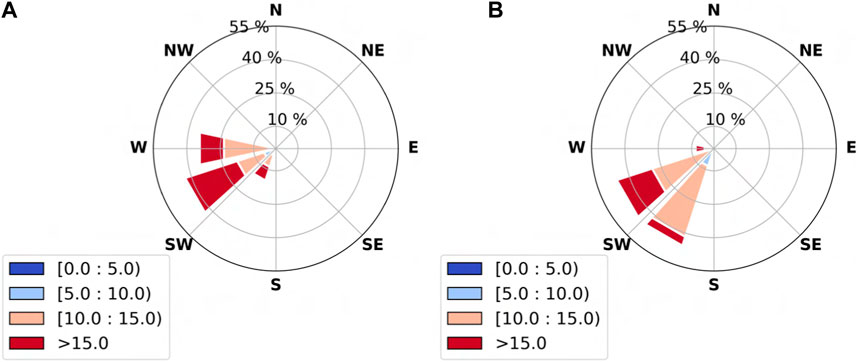
Figure 9. Windrose on 11/03/2021 at 100 m a.g.l. at the Diablerets LiDAR site from (A) LiDAR measurements and (B) the COSMO-WRF simulation. Colors represent wind speed in m/s unit.
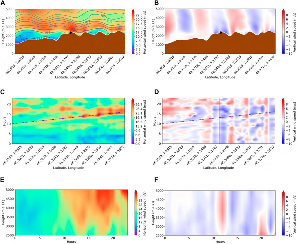
Figure 10. Vertical cross-section from COSMO-WRF on 11/03/2021, 08h00, following the orange line in Figure 1 of (A) horizontal wind speed and (B) vertical wind speed. The black dot indicates the LiDAR site. The contour lines in (A) show the potential temperature. The horizontal axis represents the latitude and longitude from west to east. The color bars in (ace) and (bdf) represent horizontal and vertical wind speeds, respectively. Red in the (B,D,F) color bar indicates upward vertical wind. Hovmoller diagram of (C) horizontal and (D) vertical wind speed at the height of 2564.90 m a.s.l. following the orange line as above. Hovmoller diagram of (E) horizontal wind speed and (F) vertical wind speed at the LiDAR location. The black vertical line in (C,D) represents the LiDAR location. The blue dashed line in (C,D) represents the propagating wave. The vertical axis of (abef) represents the height above sea level and the vertical axis of (cd) represents the hours.
Further, the Hovmoller diagram is used to present the evolution of the horizontal and vertical wind speed cross-section (x-axis) in time (y-axis) (Figures 10C, D). The Hovmoller diagram of vertical wind speed (Figure 10D) shows relatively stationary positive and negative velocity patterns, especially at the east side of the LiDAR site (black vertical line). This quasi-constant vertical velocity pattern indicates stationary mountain waves also visible in Figure 10B. The Hovmoller diagram of the horizontal wind speed shows an increase in wind speed in several areas which is interpreted as another propagating mountain wave from west to east (blue dashed line, Figure 10C). To better understand the timing of the event, another pair of Hovmoller diagrams of horizontal (Figure 10E) and vertical (Figure 10F) wind speed is provided at the location of the LiDAR. The horizontal wind speed increases at 10h00, which coincides with the downdraft wind inferred from the vertical velocity pattern, as evident in Figure 10F. This increase in wind speed might be caused by a downdraft by the mountain wave event, as described in Lehner et al. (2016).
Figure 11 shows the time series of wind speed at the Diablerets LiDAR site measured by the wind LiDAR, and simulated with COSMO-WRF and COSMO-1E. All results are hourly averaged. We notice a prominent oscillation in the LiDAR data at the wind turbine hub height, especially after 10h00. This indicates a correlation with the downdraft from the propagated wave seen from the Hovmoller diagram. The timing and amplitude of the oscillations simulated by COSMO-1E and COSMO-WRF correspond well, suggesting that COSMO-1E is suitable for providing initial data for a mountain wave simulation case. The oscillations observed during 11/03/2021 at the Diablerets LiDAR site were approximately 10 m/s, as can be seen from the COSMO-WRF simulation. The study of (Draxl et al., 2021) (Cascade Range region USA) showed that wind speed oscillations on the order of 5 m/s can already create oscillations in wind turbine power output in their case study. Therefore, we may anticipate oscillations of wind speed if a turbine is placed in a region influenced by mountain waves, such as the Diablerets region.
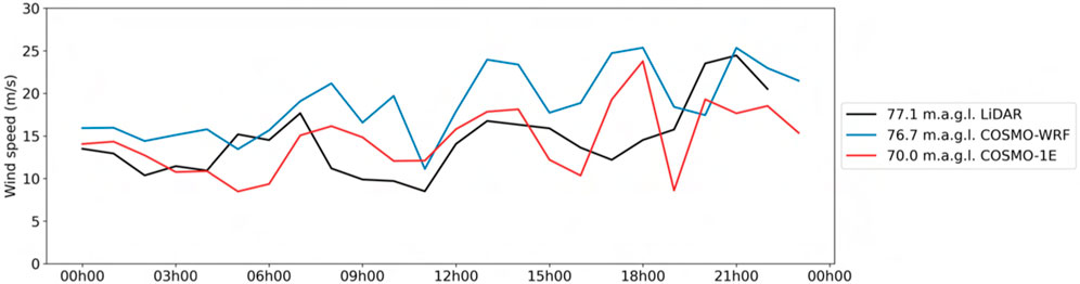
Figure 11. Hourly averaged time series of wind speed from LiDAR, COSMO-WRF, and COSMO-1E at the Diablerets LiDAR site on 11/03/2021. The color legend represents the height above ground level.
During the measurement period, the wind rose of the Diablerets site shows two predominant wind directions, i.e., southwesterly and northeasterly [as shown in Kristianti et al. (2023)]. These main wind directions are also found as the annual average using data of the Wind Atlas Switzerland (Koller and Humar, 2016). The LiDAR measurement and the COSMO-WRF simulation during the 11/03/2021 event represent a case study of a situation with a main wind direction from the Southwest (Figures 9A, B), and the Wind Atlas data indicate that this case is not an isolated but rather frequently recurring event in the Diablerets area. Cloud lines perpendicular to the southwesterly wind direction can be seen from the satellite images (Figure 7), indicating the same wind direction as seen from the LiDAR measurement and simulation result (Figures 9A, B).
COSMO-1E 2019 data is used to find the relative frequency of atmospheric conditions favoring the formation of mountain waves. We adopted the wind speed threshold and static stability used in Díaz-Fernández et al. (2022). Note that this threshold is mainly based on the atmospheric condition neglecting the topographic characteristics. The purpose of focusing only on the atmospheric conditions is to create a universal threshold that can be quickly adapted to any location in the Alpine region. As shown in Figure 7B almost the entire Swiss Alpine area may be affected by mountain waves, therefore we focus on atmospheric conditions that allow generation of mountain waves and assume spatial coverage at the scale of the Alpine region. We acknowledged that this crude estimation may lead to significant overestimation but serves here as an order of magnitude characterization to get an idea of the significance of mountain wave events.
For a mountain wave to develop, wind speed needs to be high enough to traverse the mountain ridge, otherwise flow separation or other topographic wind flow will occur instead of a wave. Following the recommendation of Reichmann (1978) and the study of Draxl et al. (2021), a wind speed aloft larger than 8 m/s would be sufficient for a mountain wave to be formed. Therefore, the first threshold is a wind speed at 1,164 m a.g.l. equal or larger than 8 m/s. The second threshold is the static stability (ST, Eq. 1) number following the equation and threshold used by Díaz-Fernández et al. (2022). For a wave to form, the static stability (ST) number is required to be between 0.0002 and 0.0014 K/Pa. T is temperature, θ is potential temperature, and p is the barometric pressure. Variable d(θ) and dp are calculated using potential temperature and pressure difference from 1,164 m a.g.l. and 10 m a.g.l. from COSMO-1E data.
The percentage of atmospheric conditions favorable for the potential formation of mountain waves is shown in Figure 12 for the Diablerets and Lukmanier LiDAR sites. Both sites show a higher percentage of favorable conditions during the winter time, covering up to 80% of the time. This result demonstrates the importance of considering mountain waves when assessing wind energy, especially, when wind energy is designed to respond to the increased winter energy demand. Both sites also show a slightly higher percentage during the first half of wintertime in October to December compared to January to March. The percentage is lower during the spring and summer seasons from April to September. However, there is still a significant number of days with the potential of mountain wave formation of approximately 40%. This might be due to the relatively high wind speed at the Diablerets and Lukmanier LiDAR sites and the stable atmospheric conditions during the night time, both leading to the defined threshold being met.
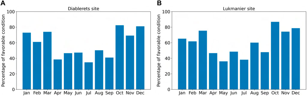
Figure 12. Time fraction (%) of conditions favorable for the occurrence of mountain waves based on the COSMO-1E 2019 data at the (A) Diablerets and (B) Lukmanier sites.
The fluctuation in wind speed related to the mountain wave event has the potential to influence wind energy production, depending on its location in the region of the power curve (Figure 2). In this paper, we are solely focusing on the impact of wind speed fluctuations and we exclude other variables related to mountain wave event that might also influence the power output (i.e. turbulence, etc). For a mountain wave to occur, it requires high wind speed, as we defined in the threshold above. Depending on the type of wind turbine, it is less likely that the fluctuation will occur in the first region, below the vcut_in. If the fluctuation occurs within the second region (between vcut_in and vrated), depending on the scale of the fluctuation amplitude, we can expect a high impact on the power output production. For stable output of power production and minimum impact of mountain wave on power production, the range of fluctuation ideally occurs within the third region (between vrated and vcut_off) but not reaching the fourth region, which in this case could lead to wind turbines not operating. The region distribution of the power curve varies between the wind turbine infrastructures. The goal of introducing the possibility of mountain wave occurrence during the planning and wind assessment process is to help the process of infrastructure selection to maximize the potential power production in the area.
Mountain wave events in the Diablerets region have been shown to influence the wind speed at the typical height of wind turbine hubs. For regions prone to a high occurrence of mountain waves, we suggest consideration of mountain waves potentially propagating down to the level of wind turbine hubs when assessing wind potential in complex Alpine terrain. In Switzerland, wintertime energy demand increases; at the same time, the stable atmospheric conditions during winter create a favorable situation for mountain waves to occur. We have shown that the percentage of favorable atmospheric conditions for wave formation is higher during the winter time up to 80% at the Lukmanier and Diablerets LiDAR sites. Further investigation is still needed to study how the downward propagation of mountain waves exactly influences wind energy production.
3.3 Influence of Foehn wind at turbine hub height
In this section, the influence of Foehn on potential wind is explored and a statistical estimation of event occurrence is provided, to support an accurate wind assessment in complex terrain. First, we provide analyses of two Foehn events in the Lukmanier domain (Figure 1, blue box) using two simulations with a southerly (23/10/2020) and northerly (09/12/2020) wind direction, respectively. Then the statistical estimation of how often Foehn events occur is provided based on meteorological measurements in the surroundings of the Lukmanier area in 2022 using the Foehnix model (Plavcan et al., 2014) (Sect. 2.2.3). Figure 13A shows the mean wind speed from COSMO-WRF on 23/10/2020 at 100 m a.g.l. in the Lukmanier domain during southerly Foehn. The simulation shows high wind speed over the lee slopes of the main mountain ridges, corresponding to the northern part of the domain. Figure 13B shows the simulated mean wind speed on 09/12/2020 during northerly Foehn. In this case, areas of high wind speed over the lee slopes are located in the southern part of the domain.
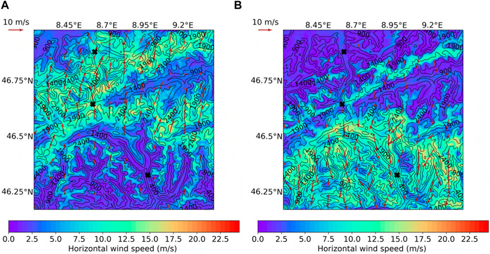
Figure 13. Daily mean wind speed from COSMO-WRF at 100 m a.g.l. in the Lukmanier region on 23/10/2020 (A) and 09/12/2020 (B). The arrows indicate the wind direction. The contour lines show the elevation above sea level in the COSMO-WRF model. The black crosses show the locations of the wind measurement stations used as input for the Foehnix model.
For further analysis, a vertical cross-section is shown in Figure 14 with the wind direction left to right and including the crest and valley in the direction of Foehn wind. For both, the northerly and southerly case, we see an increase in wind speed at the lee side of the mountain (Figures 14A, B) confirming the situation shown in Figure 13. The increase in horizontal wind speed is accompanied by an increase in temperature (Figures 14C, D) and a decrease in relative humidity (Figures 14E, F), all typical characteristics of a warm dry Foehn wind. As we see in Figure 14, the altitude affected by the Foehn event involves the height where wind turbines operate. Therefore, for wind assessment purposes in areas known to be affected by Foehn, we recommend including the frequency of Foehn occurrence for a more accurate wind assessment.
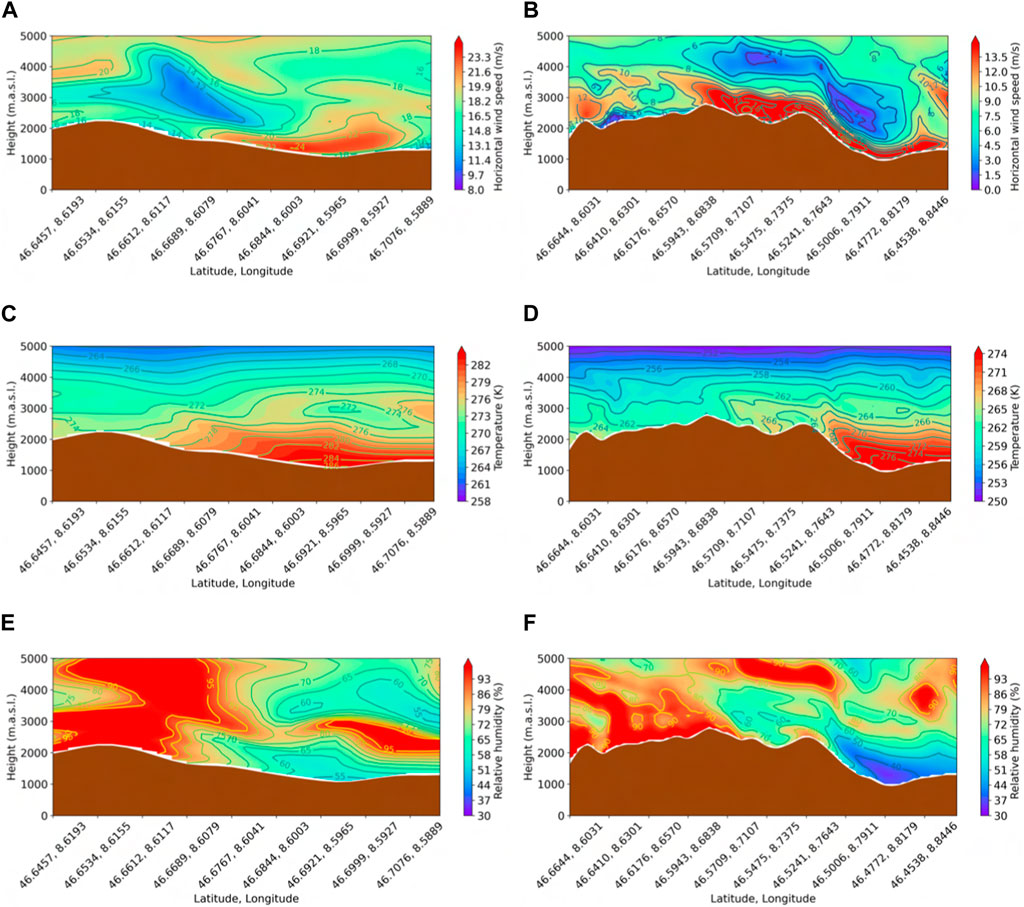
Figure 14. Vertical cross-section from COSMO-WRF on 23/10/2020, 13h00 for southerly Foehn (left) and on 09/12/2020, 09h00 for northerly Foehn (right) for (A,B) horizontal wind speed (m/s), (C,D) temperature (K), and (E,F) relative humidity (%). For the southerly Foehn event, the vertical cross-section starts from 46.64560° N, 8.61934° E (south of GUE crest station) to 46.71181° N, 8.58495° E (east side of Göschenen valley) as shown by the black line in the Lukmanier domain, Figure 1. For the northerly Foehn event, the vertical cross-section starts from 46.66363° N, 8.60292° E (northwest of GUE crest station) to 46.43380° N, 8.86705° E (along Valle Leventina) as shown by the orange line in the Lukmanier domain, Figure 1.
Applying the Foehnix model, we select the GUE crest as the central indicator station for both the northerly and southerly Foehn. BIA and ALT are selected as downwind indicator valley stations for northerly and southerly Foehn, respectively. More details of these stations can be found in Table 1 and their location is shown in Figure 1. The wind direction filter was chosen based on the wind roses of the three stations and the topography situation. Figure 15 shows the wind roses of the stations ALT, GUE, and BIA for 2022. A total number of 8,760 hourly wind speed records were utilized. ALT station shows a major wind direction from the south-southeast, while BIA presents a dominant wind direction from the north-northwest. Both stations show a secondary sector almost opposite to the respective dominant sector. GUE station, located on the crest, shows prevailing winds from both directions, north and south. Taking the local topography situation and wind direction into consideration, we pick the southeasterly as the main axis for the wind direction filter of southerly Foehn. We also pick northerly for the wind direction filter for the northerly Foehn. Hence, we applied a wind direction filter of 45°–225° and 270°–90° for southerly and northerly Foehn, respectively. The wind direction filters span within a sector of 180° following a recommendation by Plavcan et al. (2014) and is set equally for both crest and valley stations. The defined wind direction filter cluster the measured wind in the specified sectors. Then, based on air temperature difference, wind speed, and relative humidity, the Foehnix model identifies the probability of occurrence of Foehn events.
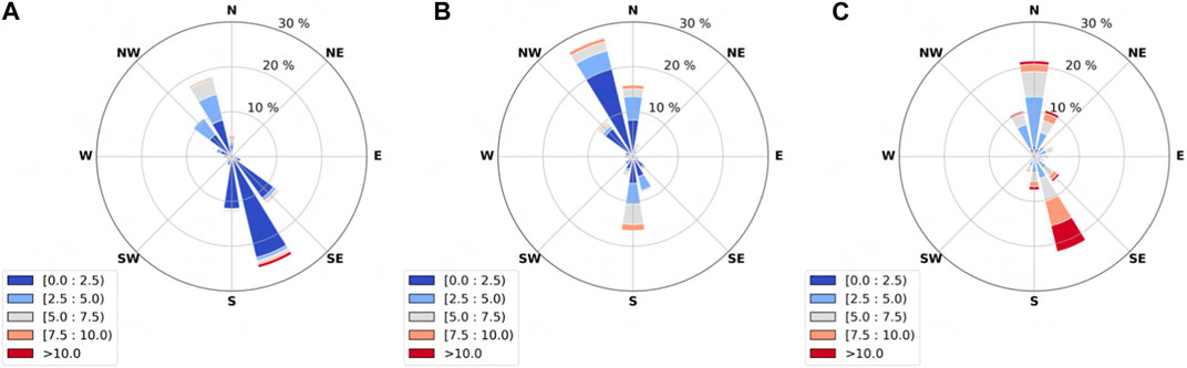
Figure 15. Wind roses for the measurement stations of (A) Altdorf (ALT), (B) Biasca (BIA), and (C) Gütsch (GUE) for the year 2022. The color bar represents wind speed (m/s).
When the estimated probability of Foehn exceeds 50%, it is assumed that a Foehn event occurs. The threshold of 50% follows the classification threshold used by Plavcan et al. (2014) The Foehnix model provides the number of hours with favorable conditions for Foehn generation (Figures 16A, B). The northerly Foehn has the highest frequency during the winter months of January and February. A similarly high frequency of northerly Foehn during winter has been reported by Meteoswiss for the Poschiavo station in eastern Switzerland from 2008 until 2020 (MeteoSwiss, 2023). This comparison is made to show the representativity of the seasonal patterns for a larger region and for a longer period of time. Poschiavo and Altdorf are some of the most representative stations for the northerly and southerly Foehn according to MeteoSwiss (2023) (Figures 16C, D). Poschiavo station, in particular, has been known for its record-high Foehn activity MeteoSwiss (2023). This can also be seen from the high hours of favorable conditions produced by the Foehnix model for the northerly Foehn (Figure 16A). The frequency of northerly Foehn from the Foehnix model varies strongly from spring to autumn 2022, while the Foehn hours from Poschiavo station are lowest from August to November. Following the Foehnix results, the southerly Foehn has the highest occurrence in March 2022. The long-term data from Altdorf shows the highest frequency in April from 1991 to 2020 (MeteoSwiss, 2023). Both show the lowest frequency during July and August. The difference between the result of the Foehnix model from measurement stations in 2022 and the long-term records from Meteoswiss can be attributed to the inter-annual variability and different locations of the stations.
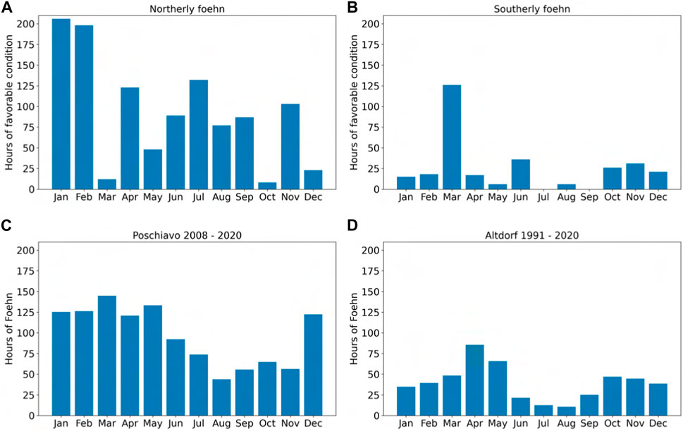
Figure 16. Number of hours of favorable conditions for (A) northerly Foehn (BIA and GUE stations) and (B) southerly Foehn (ALT and GUE stations) to occur based on the Foehnix model using measurements of 2022. Number of hours of (C) northerly Foehn at Poschiavo from 2008 to 2020, and (D) southerly Foehn at Altdorf from 1991 to 2020 (MeteoSwiss, 2023).
The Foehn event increases the wind speed significantly in the valley region and has a high probability to be higher than the vcut_off (fourth region, Figure 2). Therefore, wind assessment in the area with a high probability of Foehn occurrence should be done thoroughly. The benefit of including the Foehn event in the wind assessment is not only for a better selection of appropriate infrastructure but also to give us a better picture of the future potential production of wind turbines. With the right infrastructure, a wind turbine could handle the high wind speed event of Foehn and reduce the number of nonoperational wind turbines. Even when the Foehn event still results in a non-operational wind turbine, including it in the assessment process will improve the accuracy of the production forecast. A high number of hours of Foehn as seen in Figure 16 should be taken into consideration, especially if the goal is to fulfill the energy demand during the wintertime. The warm dry high wind speed produced by the Foehn event can also reduce the icing issue for the wind turbine during the wintertime. For the installation of wind turbines in a remote complex terrain area, this would mean less maintenance needed.
Foehn has been shown to increase the wind speed on the lee slopes in the Lukmanier domain. Results from an analysis of historical Foehn data from Meteoswiss, together with model predictions based on data measured in 2022 show a significantly higher frequency of Foehn events especially during the winter (northerly Foehn) and spring season (southerly Foehn), strengthening the motivation to include Foehn analysis in wind power assessments with the objective to reduce the energy production gap during the winter season. More research is needed to quantify the impact of Foehn on turbine power yields, the impact of turbulence, and to develop better forecasts for accurate wind speed assessment.
4 Conclusion
For providing the most advanced assessment of wind potential in complex mountain terrain, it is necessary to improve our understanding and the modeling of topography-induced effects on wind. This paper presents examples of terrain effects on wind in the Swiss Alps, namely mountain waves and Foehn, and estimates the occurrence of these phenomena. Two field measurement campaigns were conducted in the Lukmanier and Diablerets areas of the Swiss Alps collecting wind data using a Doppler wind LiDAR instrument. The COSMO-WRF model is used to investigate meteorological events that led to stronger wind at the mountain tops and the typical height of wind turbine hubs during the field measurements. The numerical simulations with COSMO-WRF using wind data from measurement stations located in the model domain show an improvement in wind speed representation near ground level in complex mountain terrain. However, modeled high-resolution wind further aloft is mainly driven by the input data, COSMO-1E, which shows an overestimation compared to the LiDAR measurement data. More realistic input data is needed for a more accurate simulation of wind at higher altitudes.
Mountain waves and Foehn are investigated as examples of meteorological phenomena that happen in Alpine complex terrain with significant impact for the wind energy production, especially during winter. Mountain waves occur during stable atmospheric conditions which are more prevalent in winter, when the demand of energy is high. Our study shows that the wind speed fluctuations associated with mountain waves can propagate downward to the height above ground where the wind turbines typically operate, i.e., 100 m. Further study on the frequency of events and the downward propagation process is still needed for an accurate assessment of wind speed in complex terrain.
The simulation of Foehn events in the Lukmanier area shows that such winds may have a strong effect at the level where the wind turbines operate. Using the Foehnix model, we estimated the probability of Foehn occurrence, which was found higher during winter and early springtime than during summer and fall. This information is useful for establishing a more accurate assessment of wind power potential in complex terrain. This finding adds the significance of including the Foehn assessment for accurate wind prediction in the Alpine complex terrain. The performed measurements, simulations, and analyses enable an improved accuracy of wind assessment especially during winter by considering prominent characteristic flow features and the meteorological conditions favoring their genesis and occurrence. This underlines the dominant influence of the local terrain and topography on the wind speed and wind direction and thus on potential wind power production by turbines deployed at selected favorable sites for that purpose.
This study underlines the need for sufficiently detailed assessment, including the near surface effects such as through Foehn and mountain waves, to assess their quantitative impact on the potential power production of wind turbines in the Swiss mountains. The future study will include a more in-depth analysis of the complex terrain phenomenon mechanism in the Swiss Alps region, such as analysis for the area of impact and a more solid recommendation for wind energy community in the area with a high probability of mountain wave and Foehn cases. Due to the limited data availability during our measurement campaign, we have a limited number of cases to investigate. A longer and more thorough campaign will help to add more cases to investigate and create a more generalized conclusion. It might also discover more examples of complex terrain phenomenon which have impacts on wind energy, other than mountain waves and Foehn. Integrating the information on the impact of complex terrain phenomenon with machine learning [i.e. Dujardin and Lehning (2022)] and Digital Twin and its integration to Geographical Information System (GIS) (Agostinelli et al., 2022; Yousef et al., 2023; Piras et al., 2024) will also increase the accuracy of monitoring and performance prediction of wind turbines. The present research acts as a step forward in accurately estimating potential wind power and optimally using it for renewable energy production, particularly during periods when it is most needed, i.e., the winter season when power demand is high and other renewable sources are limited.
Data availability statement
The data presented in the study are deposited in the EnviDat repository and can be found at https://www.doi.org/10.16904/envidat.501.
Author contributions
FK: Writing–original draft, Conceptualization, Investigation, Software, Writing–review and editing. FG: Software, Investigation, Writing–review and editing. SG-H: Validation, Visualization, Writing–review and editing. JD: Writing–review and editing. HH: Investigation, Writing–review and editing. SH: Writing–review and editing. ML: Supervision, Project Administration, Funding acquisition, Conceptualization, Writing–review and editing.
Funding
The author(s) declare that financial support was received for the research, authorship, and/or publication of this article. The research published in this publication was carried out with the support of the Swiss Federal Office of Energy as part of the SWEET consortium EDGE, Swiss National Science Foundation (SNSF): Grant 179130, and the Swiss National Supercomputing Centre (CSCS) projects s938, s1115 and s1242. The authors bear sole responsibility for the conclusions and the results presented in this publication.
Acknowledgments
We acknowledge the use of imagery from the Worldview Snapshots application (https://wvs.earthdata.nasa.gov), part of the Earth Observing System Data and Information System (EOSDIS). We thank Glacier3000, Planair, MeteoSwiss, Swiss Federal Department of Defence, Civil Protection and Sport, and Halo Photonics Online support for data provisions, collaborations, and logistical support of the field campaigns.
Conflict of interest
The authors declare that the research was conducted in the absence of any commercial or financial relationships that could be construed as a potential conflict of interest.
The author(s) declared that they were an editorial board member of Frontiers, at the time of submission. This had no impact on the peer review process and the final decision.
Publisher’s note
All claims expressed in this article are solely those of the authors and do not necessarily represent those of their affiliated organizations, or those of the publisher, the editors and the reviewers. Any product that may be evaluated in this article, or claim that may be made by its manufacturer, is not guaranteed or endorsed by the publisher.
References
Agostinelli, S., Cumo, F., Nezhad, M. M., Orsini, G., and Piras, G. (2022). Renewable energy system controlled by open-source tools and digital twin model: zero energy port area in Italy. Energies 15, 1817. doi:10.3390/en15051817
Alfredsson, P.-H., and Segalini, A. (2017). Introduction wind farms in complex terrains: an introduction. Philosophical Trans. R. Soc. A Math. Phys. Eng. Sci. 375, 20160096. doi:10.1098/rsta.2016.0096
Archer, C. L., and Jacobson, M. Z. (2005). Evaluation of global wind power. J. Geophys. Res. Atmos. 110. doi:10.1029/2004JD005462
Archer, C. L., and Jacobson, M. Z. (2013). Geographical and seasonal variability of the global “practical” wind resources. Appl. Geogr. 45, 119–130. doi:10.1016/j.apgeog.2013.07.006
Bavay, M., Lehning, M., Jonas, T., and Löwe, H. (2009). Simulations of future snow cover and discharge in alpine headwater catchments. Hydrol. Process. 23, 95–108. doi:10.1002/hyp.7195
Beffrey, G., Jaubert, G., and Dabas, A. (2006). Föhn flow and stable air mass in the rhine valley: the beginning of a map event. Q. J. R. Meteorological Soc. 130, 541–560. doi:10.1256/qj.02.228
Beljaars, A. C. (1995). The parametrization of surface fluxes in large-scale models under free convection. Q. J. R. Meteorological Soc. 121, 255–270. doi:10.1256/smsqj.52202
Chow, F. K., Schär, C., Ban, N., Lundquist, K. A., Schlemmer, L., and Shi, X. (2019). Crossing multiple gray zones in the transition from mesoscale to microscale simulation over complex terrain. Atmosphere 10, 274. doi:10.3390/atmos10050274
Chow, F. K., Snyder, B. J., and Wekker, S. F. J. D. (2013). Mountain weather research and forecasting: recent progress and current challenges. Mt. Weather Res. Forecast. doi:10.1007/978-94-007-4098-3
Clark, R. T., Bett, P. E., Thornton, H. E., and Scaife, A. A. (2017). Skilful seasonal predictions for the european energy industry. Environ. Res. Lett. 12, 024002. doi:10.1088/1748-9326/aa57ab
Clifton, A., Barber, S., Stökl, A., Frank, H., and Karlsson, T. (2022). Research challenges and needs for the deployment of wind energy in hilly and mountainous regions. Wind Energy Sci. 7, 2231–2254. doi:10.5194/wes-7-2231-2022
Clifton, A., Daniels, M., and Lehning, M. (2014). Effect of winds in a mountain pass on turbine performance. Wind Energy 17, 1543–1562. doi:10.1002/we.1650
Dar, A. S., Berg, J., Troldborg, N., and Patton, E. G. (2019). On the self-similarity of wind turbine wakes in a complex terrain using large eddy simulation. Wind Energy Sci. 4, 633–644. doi:10.5194/wes-4-633-2019
Dhunny, A., Lollchund, M., and Rughooputh, S. (2017). Wind energy evaluation for a highly complex terrain using computational fluid dynamics (cfd). Renew. Energy 101, 1–9. doi:10.1016/j.renene.2016.08.032
Díaz-Fernández, J., Bolgiani, P., Santos-Muñoz, D., Quitián-Hernández, L., Sastre, M., Valero, F., et al. (2022). Comparison of the wrf and harmonie models ability for mountain wave warnings. Atmos. Res. 265, 105890. doi:10.1016/j.atmosres.2021.105890
Draxl, C., Worsnop, R. P., Xia, G., Pichugina, Y., Chand, D., Lundquist, J. K., et al. (2021). Mountain waves can impact wind power generation. Wind Energy Sci. 6, 45–60. doi:10.5194/wes-6-45-2021
Dujardin, J., Kahl, A., Kruyt, B., Bartlett, S., and Lehning, M. (2017). Interplay between photovoltaic, wind energy and storage hydropower in a fully renewable Switzerland. Energy 135, 513–525. doi:10.1016/j.energy.2017.06.092
Dujardin, J., Kahl, A., and Lehning, M. (2021). Synergistic optimization of renewable energy installations through evolution strategy. Environ. Res. Lett. 16, 064016. doi:10.1088/1748-9326/abfc75
Dujardin, J., and Lehning, M. (2022). Wind-topo: downscaling near-surface wind fields to high-resolution topography in highly complex terrain with deep learning. Q. J. R. Meteorological Soc. 148, 1368–1388. doi:10.1002/qj.4265
Dyer, A., and Hicks, B. (1970). Flux-gradient relationships in the constant flux layer. Q. J. R. Meteorological Soc. 96, 715–721. doi:10.1002/qj.49709641012
Elgendi, M., AlMallahi, M., Abdelkhalig, A., and Selim, M. Y. (2023). A review of wind turbines in complex terrain. Int. J. Thermofluids 17, 100289. doi:10.1016/j.ijft.2023.100289
ESRI (2023). World imagery. Available at: https://www.arcgis.com/home/item.html?id=10df2279f9684e4a9f6a7f08febac2a9 (Accessed November 13, 2023).
European Environmental Agency (2006). CORINE land cover (CLC) 2006 raster data,Version 13. Available at: https://www.eea.europa.eu/dataand-maps/data/clc-2006-raster (Accessed May 28, 2021).
Federal Office of Meteorology and Climatology MeteoSwiss (2023a). Cosmo forecasting system. Available at: https://www.meteoswiss.admin.ch/weather/warning-and-forecasting-systems/cosmo-forecasting-system.html (Accessed January 4, 2023).
Federal Office of Meteorology and Climatology MeteoSwiss (2023b) Measurement instruments. Available at: https://www.meteoswiss.admin.ch/weather/measurement-systems/land-based-stations/automatic-measurement-network/measurement-instruments.html (Accessed February 9, 2023).
Federal Office of Topography (2023). Swiss map raster. Available at: https://map.geo.admin.ch/ (Accessed May 23, 2023).
GADM (2022). GADM version 4.1. Available at: https://geodata.ucdavis.edu/gadm/ (Accessed November 21, 2023).
Gerber, F., Besic, N., Sharma, V., Mott, R., Daniels, M., Gabella, M., et al. (2018). Spatial variability in snow precipitation and accumulation in cosmo–wrf simulations and radar estimations over complex terrain. Cryosphere 12, 3137–3160. doi:10.5194/tc-12-3137-2018
Gerber, F., and Lehning, M. (2021). High resolution static data for WRF over Switzerland. Tech. rep.
Gerber, F., and Sharma, V. (2018) Running cosmo-wrf on very-high resolution over complex terrain. doi:10.16904/envidat.35
Graabak, I., and Korpås, M. (2016). Variability characteristics of european wind and solar power resources—a review. Energies 9, 449. doi:10.3390/en9060449
Grams, C. M., Beerli, R., Pfenninger, S., Staffell, I., and Wernli, H. (2017). Balancing europe’s wind-power output through spatial deployment informed by weather regimes. Nat. Clim. Change 7, 557–562. doi:10.1038/nclimate3338
Kealy, J. C., Efstathiou, G. A., and Beare, R. J. (2019). The onset of resolved boundary-layer turbulence at grey-zone resolutions. Boundary-Layer Meteorol. 171, 31–52. doi:10.1007/s10546-018-0420-0
Klemp, J. B., Dudhia, J., and Hassiotis, A. D. (2008). An upper gravity-wave absorbing layer for nwp applications. Mon. Weather Rev. 136, 3987–4004. doi:10.1175/2008MWR2596.1
Koletsis, I., Lagouvardos, K., Kotroni, V., and Bartzokas, A. (2009). The interaction of northern wind flow with the complex topography of crete island – part 1: observational study. Nat. Hazards Earth Syst. Sci. 9, 1845–1855. doi:10.5194/nhess-9-1845-2009
Koletsis, I., Lagouvardos, K., Kotroni, V., and Bartzokas, A. (2010). The interaction of northern wind flow with the complex topography of crete island – part 2: numerical study. Nat. Hazards Earth Syst. Sci. 10, 1115–1127. doi:10.5194/nhess-10-1115-2010
Koller, S., and Humar, T. (2016) Windpotentialanalyse für windatlas.ch: Jahresmittelwerte der modellierten windgeschwindigkeit und windrichtung.
Kristianti, F., Dujardin, J., Gerber, F., Huwald, H., Hoch, S. W., and Lehning, M. (2023). Combining weather station data and short-term lidar deployment to estimate wind energy potential with machine learning: a case study from the swiss alps. Boundary-Layer Meteorol. 188, 185–208. doi:10.1007/s10546-023-00808-y
Kristianti, F., Gerber, F., and Lehning, M. (2024) Cosmo-wrf dataset for swiss alps simulations in gray-zone resolution. doi:10.16904/envidat.501
Kruyt, A. C. (2019). Potential and uncertainty of wind energy in the swiss alps. EPFL thesis, 126. doi:10.5075/epfl-thesis-9350
Kruyt, B., Dujardin, J., and Lehning, M. (2018). Improvement of wind power assessment in complex terrain: the case of cosmo-1 in the swiss alps. Front. Energy Res. 6, 102. doi:10.3389/fenrg.2018.00102
Lange, J., Mann, J., Berg, J., Parvu, D., Kilpatrick, R., Costache, A., et al. (2017). For wind turbines in complex terrain, the devil is in the detail. Environ. Res. Lett. 12, 094020. doi:10.1088/1748-9326/aa81db
Lehner, M., and Rotach, M. W. (2018). Current challenges in understanding and predicting transport and exchange in the atmosphere over mountainous terrain. Atmosphere 9, 276. doi:10.3390/atmos9070276
Lehner, M., Whiteman, C. D., Hoch, S. W., Crosman, E. T., Jeglum, M. E., Cherukuru, N. W., et al. (2016). The metcrax ii field experiment: a study of downslope windstorm-type flows in Arizona’s meteor crater. Bull. Am. Meteorological Soc. 97, 217–235. doi:10.1175/BAMS-D-14-00238.1
Lehning, M., Doorschot, J., and Bartelt, P. (2000). A snowdrift index based on snowpack model calculations. Ann. Glaciol. 31, 382–386. doi:10.3189/172756400781819770
Mann, J., Angelou, N., Arnqvist, J., Callies, D., Cantero, E., Arroyo, R. C., et al. (2017). Complex terrain experiments in the new european wind atlas. Philosophical Trans. Ser. A, Math. Phys. Eng. Sci. 375, 20160101. doi:10.1098/rsta.2016.0101
MeteoSwiss (2022) Meteoswiss idaweb. Available at: https://gate.meteoswiss.ch/idaweb/ (Last access: 2022.
MeteoSwiss (2023). Foehn frequency. Available at: https://www.meteoswiss.admin.ch/weather/weather-and-climate-from-a-to-z/foehn-frequency.html (Accessed November 6, 2023).
Mlawer, E. J., Taubman, S. J., Brown, P. D., Iacono, M. J., and Clough, S. A. (1997). Radiative transfer for inhomogeneous atmospheres: rrtm, a validated correlated-k model for the longwave. J. Geophys. Res. Atmos. 102, 16663–16682. doi:10.1029/97jd00237
Morrison, H., Thompson, G., and Tatarskii, V. (2009). Impact of cloud microphysics on the development of trailing stratiform precipitation in a simulated squall line: comparison of one-and two-moment schemes. Mon. weather Rev. 137, 991–1007. doi:10.1175/2008mwr2556.1
NASA EARTHDATA (2023). EOSDIS Worldview. Available at: https://worldview.earthdata.nasa.gov/ (Accessed November 13, 2023).
NASA/METI/AIST/Japan Space systems and U.S./Japan ASTER Science Team (2019). ASTER global digital elevation model V003, NASA EOSDIS Land Process. DAAC, Distrib. by NASA EOSDIS Land Process. DAAC. doi:10.5067/ASTER/ASTGTM.003
Niu, G.-Y., Yang, Z.-L., Mitchell, K. E., Chen, F., Ek, M. B., Barlage, M., et al. (2011). The community noah land surface model with multiparameterization options (noah-mp): 1. model description and evaluation with local-scale measurements. J. Geophys. Res. Atmos. 116, D12109. doi:10.1029/2010jd015139
Olabi, A., and Abdelkareem, M. A. (2022). Renewable energy and climate change. Renew. Sustain. Energy Rev. 158, 112111. doi:10.1016/j.rser.2022.112111
Paulson, C. A. (1970). The mathematical representation of wind speed and temperature profiles in the unstable atmospheric surface layer. J. Appl. Meteorology Climatol. 9, 857–861. doi:10.1175/1520-0450(1970)009<0857:tmrows>2.0.co;2
Pickering, B., Grams, C. M., and Pfenninger, S. (2020). Sub-national variability of wind power generation in complex terrain and its correlation with large-scale meteorology. Environ. Res. Lett. 15, 044025. doi:10.1088/1748-9326/ab70bd
Piras, G., Agostinelli, S., and Muzi, F. (2024). Digital twin framework for built environment: a review of key enablers. Energies 17, 436. doi:10.3390/en17020436
Plavcan, D., Mayr, G. J., and Zeileis, A. (2014). Automatic and probabilistic foehn diagnosis with a statistical mixture model. J. Appl. Meteorology Climatol. 53, 652–659. doi:10.1175/jamc-d-13-0267.1
Schraff, C., Reich, H., Rhodin, A., Schomburg, A., Stephan, K., Periáñez, A., et al. (2016). Kilometre-scale ensemble data assimilation for the cosmo model (kenda). Q. J. R. Meteorological Soc. 142, 1453–1472. doi:10.1002/qj.2748
Shin, H. H., and Hong, S.-Y. (2015). Representation of the subgrid-scale turbulent transport in convective boundary layers at gray-zone resolutions. Mon. Weather Rev. 143, 250–271. doi:10.1175/mwr-d-14-00116.1
Sims, R. (2004). Renewable energy: a response to climate change. Sol. Energy 76, 9–17. Solar World Congress 2001. doi:10.1016/S0038-092X(03)00101-4
Skamarock, W., Klemp, J., Dudhia, J., Gill, D., Barker, D., Wang, W., et al. (2008) A description of the advanced research wrf version 3 27, 3–27.
Skamarock, W., Klemp, J. B., Dudhia, J., Gill, D. O., Liu, Z., Berner, J., et al. (2021) A description of the advanced research wrf model version 4.3. doi:10.5065/1dfh-6p97
Swiss Federal Office of Energy (2023a). Energy consumption in Switzerland 2021. Available at: https://www.bfe.admin.ch/bfe/en/home/supply/statistics-and-geodata/energy-statistics/overall-energy-statistics.html/ (Accessed May 30, 2023).
Swiss Federal Office of Energy (2023b) Energy perspectives 2050+. Available at: https://www.bfe.admin.ch/bfe/en/home/policy/energy-perspectives-2050-plus.html (Accessed May 30, 2023).
Tabas, D., Fang, J., and Porté-Agel, F. (2019). Wind energy prediction in highly complex terrain by computational fluid dynamics. Energies 12, 1311. doi:10.3390/en12071311
Tobin, I., Vautard, R., Balog, I., Bréon, F.-M., Jerez, S., Ruti, P., et al. (2015). Assessing climate change impacts on European wind energy from ENSEMBLES high-resolution climate projections. Clim. Change 128, 99–112. doi:10.1007/s10584-014-1291-0
Toumelin, L. L., Gouttevin, I., Helbig, N., Galiez, C., Roux, M., and Karbou, F. (2023). Emulating the adaptation of wind fields to complex terrain with deep learning. Artif. Intell. Earth Syst. 2, e220034. doi:10.1175/aies-d-22-0034.1
Udina, M., Bech, J., Gonzalez, S., Soler, M. R., Paci, A., Miró, J. R., et al. (2020). Multi-sensor observations of an elevated rotor during a mountain wave event in the eastern pyrenees. Atmos. Res. 234, 104698. doi:10.1016/j.atmosres.2019.104698
Webb, E. K. (1970). Profile relationships: the log-linear range, and extension to strong stability. Q. J. R. Meteorological Soc. 96, 67–90. doi:10.1002/qj.49709640708
WSL SLF (2022) Wsl slf institute for snow and avalanche research. Available at: https://www.slf.ch/en/avalanche-bulletin-and-snow-situation/measured-values/description-of-automated-stations.html (Last access: 2022.
Wyngaard, J. C. (2004). Toward numerical modeling in the “terra incognita”. J. Atmos. Sci. 61, 1816–1826. doi:10.1175/1520-0469(2004)061⟨1816:TNMITT⟩2.0.CO;2
Xia, G., Draxl, C., Raghavendra, A., and Lundquist, J. K. (2021). Validating simulated mountain wave impacts on hub-height wind speed using sodar observations. Renew. Energy 163, 2220–2230. doi:10.1016/j.renene.2020.10.127
Yang, Z.-L., Niu, G.-Y., Mitchell, K. E., Chen, F., Ek, M. B., Barlage, M., et al. (2011). The community noah land surface model with multiparameterization options (noah-mp): 2. evaluation over global river basins. J. Geophys. Res. Atmos. 116, D12110. doi:10.1029/2010jd015140
Yousef, L. A., Yousef, H., and Rocha-Meneses, L. (2023). Artificial intelligence for management of variable renewable energy systems: a review of current status and future directions. Energies 16, 8057. doi:10.3390/en16248057
Keywords: wind energy, mountain wave, leewave, complex terrain, Foehn, lidar
Citation: Kristianti F, Gerber F, Gonzàlez-Herrero S, Dujardin J, Huwald H, Hoch SW and Lehning M (2024) Influence of air flow features on alpine wind energy potential. Front. Energy Res. 12:1379863. doi: 10.3389/fenrg.2024.1379863
Received: 31 January 2024; Accepted: 25 April 2024;
Published: 24 May 2024.
Edited by:
Xun Shen, Osaka University, JapanReviewed by:
Giuseppe Piras, Sapienza University of Rome, ItalyAlan Wai Hou Lio, Technical University of Denmark, Denmark
Copyright © 2024 Kristianti, Gerber, Gonzàlez-Herrero, Dujardin, Huwald, Hoch and Lehning. This is an open-access article distributed under the terms of the Creative Commons Attribution License (CC BY). The use, distribution or reproduction in other forums is permitted, provided the original author(s) and the copyright owner(s) are credited and that the original publication in this journal is cited, in accordance with accepted academic practice. No use, distribution or reproduction is permitted which does not comply with these terms.
*Correspondence: Fanny Kristianti, ZmFubnkua3Jpc3RpYW50aUBlcGZsLmNo