Multi-timescale available flexibility assessment of integrated energy systems considering different proportions of wind power installations

The available flexibility capacity of the integrated energy system can be used as one of the indicators of proportions of system wind power installations, which, in turn, affects the maximum installed capacity of the system wind power, and this paper proposes a method for assessing the available flexibility of the integrated energy system at multiple timescales considering different proportions of system wind power installations. First, the framework of the integrated energy system is constructed, and based on the coupling relationship between the electrical and thermal systems, the mathematical models of the P2G, combined heat and power (CHP), energy storage equipment, and wind power generation equipment within the integrated energy system are established, and the Monte Carlo method is used to predict the wind power output in a typical scenario. Second, an integrated energy system optimization model is constructed to obtain the optimal dispatch operation of the system; the empirical mode decomposition (EMD) algorithm is used to decompose the flexibility demand curve of the system in multiple timescales. The flexibility supply capacity model of different types of flexibility resources in the system at different timescales is established, and through the comparative analysis of flexibility supply and demand at the same timescale, the upward and downward flexibility shortage probability and shortage expectation indexes at each timescale can be intuitively calculated and then weighted to constitute a comprehensive index of system flexibility assessment. Finally, the available flexibility analysis of the integrated energy system under different installed wind power capacities shows that the proposed methodology can more comprehensively assess the available flexibility capacity of the integrated energy system under different timescales, and the maximum installed wind power capacity that the system can withstand can be obtained while guaranteeing sufficient available flexibility capacity.

1 Introduction

With the shortage of fossil energy supply and increasing environmental pollution, the proportion of renewable energy generation represented by wind power and photovoltaics has been increasing (Yewei et al., 2021). However, wind and light output power are volatile, intermittent, and random, and their superposition with the volatility of the original load leads to increased fluctuations in the net load of the system (Qin and Bri-Mathias, 2017). Therefore, there is a need to vigorously develop flexibility resources and improve system flexibility to mitigate power fluctuations and insufficient ramp caused by net load changes (Jiang et al., 2022), which would otherwise bring about problems such as wind abandonment, light abandonment, and load shedding, affecting the safe and stable operation of the system. Therefore, the assessment of the available flexibility of the integrated energy system at multiple timescales with different installed wind power capacities can clarify the potential of the system’s available flexibility, which is extremely important for the subsequent planning and configuration schemes of the integrated energy system.

In order to reduce the impact of uncertainty of renewable energy output such as wind power, domestic and foreign researchers and scholars have studied the assessment of power system flexibility and the optimal allocation of flexibility resources. Yewei et al. (2021) proposed a new flexibility evaluation method for active distribution network nodes for soft normally open point integration with respect to the uncertainty of active distribution networks. Xiaoou (2020) investigated the evaluation of distribution system flexibility considering the interaction between electric vehicles and the grid. First, it analyzes charging and discharging control strategies for electric vehicles to reduce the impact of renewable energy output fluctuations on distribution system flexibility. Second, it models the battery capacity, driving schedule, and transportation network to study the impact of EV grid integration on distribution network flexibility; again, it proposes a distribution network flexibility evaluation method based on the feasibility analysis of uncertain regions. Lusha et al. (2022) proposed a coordinated evaluation methodology to determine the optimal utilization of electric vehicle time flexibility without compromising the owner’s usage of the electric vehicle. At the distribution layer, the distribution system operator first evaluates the operational boundaries of the electric vehicle aggregator to develop distribution layer services. Alireza et al. (2024) presented a methodology for obtaining maximum and minimum daily load profiles, introduced new hourly and daily system flexibility metrics, and developed a generalized methodology for quantifying and formulating system flexibility, i.e., the possible increase or decrease in power within operating constraints. All of the above studies consider the optimal allocation of flexibility resources from a single aspect such as power supply and energy storage. However, flexibility resources involve the power supply side, demand side, grid side, and energy storage side, and the selection and construction of flexibility indicators in the existing studies focus on power flexibility indicators, with less consideration given to the impacts of the thermal system and natural gas system on flexibility.

Integrated energy system flexibility extends from power system flexibility (Jiangxuan et al., 2023), but there is insufficient research on integrated energy system flexibility and the optimal allocation of flexibility resources. In recent years, domestic and foreign scholars have tried to provide a definition of integrated energy system flexibility, starting from the perspective of gas and heat systems for power systems, etc. Yufei et al. (2021) proposed a flexibility evaluation structure that can effectively evaluate the power system flexibility considering the influence of multi-energy coupling in order to fully utilize the flexibility resources and improve the operation economy. Zening et al. (2021) considered detailed building thermal dynamics and worker mobility behavior as a way to improve system flexibility by scheduling office buildings equipped with HVAC systems and electric vehicle charging piles to participate in active distribution grid optimization. Yuan et al. (2021), in order to fully utilize the flexibility potential of the cogeneration system, divided the system and the energy supply process from the perspective of flexibility analysis and proposed a new type of operation strategy that follows the flexibility of the system for energy scheduling. Jiaying et al. (2020) took the heat transfer flexibility of the urban heating system (UHS) as the research object. The concept of heating system flexibility was proposed to represent the ability of the UHS to meet the heating demand under different operating conditions in the heating season, and a corresponding evaluation method was given. Jia et al. (2021) initially proposed the definition of the safe operating region of a thermoelectric integrated energy system under the exact AC current model and non-linear heating equation in order to facilitate the safety assessment of the integrated energy system. Yue et al. (2022) proposed a multi-stage flexible planning method for regional electrical–thermal integration that takes into account the medium- and long-term dynamic characteristics. Most of the above research is aimed at assessing the flexibility of integrated energy systems, and the existing studies mainly reflect the flexibility of integrated energy systems at a particular scale, and it is difficult to quantitatively assess the flexibility at several different timescales at the same time.

In order to comprehensively consider the correspondence between flexibility demand and flexibility resources on multiple timescales, the multi-timescale scheduling method proposed by Yuxiao et al. (2021) takes into account the inertia of key inertial components, such as heat grids and combined heat and power (CHP) units, aiming at realizing the coordinated scheduling of the integrated energy system and improving the accuracy of its flexibility description. In the work of Xiaolin et al. (2022), for the characteristics of different timescale flexibility resources on the generation side, the response time of the standby flexibility capacity is divided into minutes and seconds, and the scheduling strategy of standby flexibility capacity in different timescales is proposed. The multi-timescale optimization model improves the safe operation capability of the system to a certain extent but does not take into account the instantaneous response capability of the power system and the delayed response characteristics of the thermal and natural gas systems, which may have adverse effects on the actual operation. Fugui et al. (2023) proposed a multi-timescale operation optimization strategy for integrated energy systems that takes into account equipment response characteristics and combines multiple forms of integrated demand response. None of these studies takes into account system flexibility.

To address the above issues, this paper proposes a multi-timescale available flexibility assessment process for integrated energy systems based on an empirical mode decomposition algorithm. First, the framework structure of the integrated energy system is constructed, and according to the coupling relationship among the three electrical and thermal subsystems, the mathematical models of the P2G, CHP, energy storage system, and wind power generation equipment within the integrated energy system are established, and the Monte Carlo method is used to predict the wind power output under typical scenarios. Second, a day-ahead energy market optimization model based on a general mathematical model of the integrated energy system is constructed to obtain the day-ahead optimal dispatch operation of the system. Finally, an empirical mode algorithm is used to decompose the flexibility demand curve of the system in multiple timescales. We establish the regulation capacity model of the different types of controllable units in the system under different regulation rate intervals to form multi-timescale flexibility resources, and through the matching analysis of flexibility resources and demand under the same timescale, the upward and downward flexibility deficiency probability and deficiency expectation indexes of each timescale can be calculated simply and intuitively and then weighted to form a comprehensive index for system flexibility assessment.

2 Integrated energy system framework and modeling

2.1 Integrated energy system framework

The integrated energy system takes the traditional electric power system as the core and utilizes various renewable resources such as wind and gas to integrate the cooling/heating and gas supply systems, thus realizing the synergistic supply of cooling, heat, electricity, and gas. A typical integrated energy system can be categorized into the energy supply side, energy conversion equipment, energy storage devices, energy transmission and distribution systems, and user terminals, as shown in Figure 1.

FIGURE 1

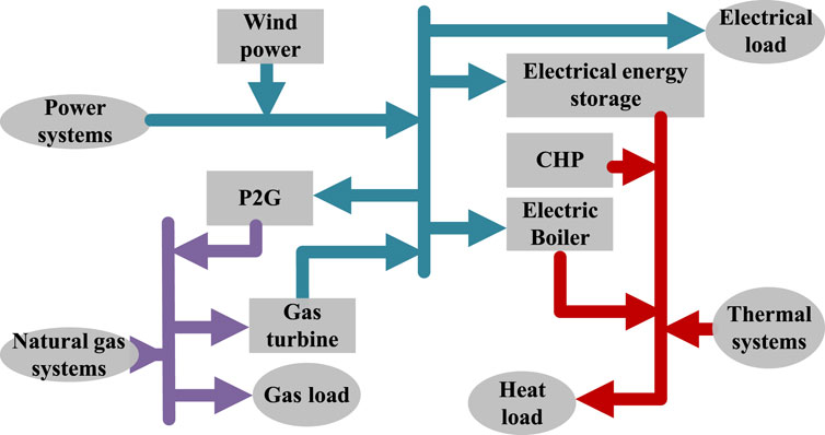
FIGURE 1. Integrated energy system framework diagram.

2.2 Integrated energy system network modeling

2.2.1 Power network modeling

Based on the analysis of the nodes of the network as well as the loop equations, the grid in the integrated energy system is modeled (Wenkai et al., 2023), and the active power P_i and the reactive power Q_i at the nodes are expressed as follows:

$P_i=V_i{\displaystyle \sum _{j=1}^n}{V}_j\left(G_{ij}\cos {\delta }_{ij}+B_{ij}\sin {\delta }_{ij}\right),(1)$

$Q_i=V_i{\displaystyle \sum _{j=1}^n}{V}_j\left(G_{ij}\sin {\delta }_{ij}-B_{ij}\cos {\delta }_{ij}\right),(2)$

where V_i and V_j are the voltages at node i and node j, respectively; δ_ij is the difference between the phase angles of the two nodes; and G_ij and B_ij are the conductance and conductance between node i and node j, respectively.

2.2.2 Natural gas network modeling

Modeling of natural gas networks in integrated energy systems involves parameters such as pressure, mass, and velocity, which are determined by the length and time of the pipeline. Comparing the mathematical models developed for various types of natural gas networks, in order to simplify the model [16], this paper does not consider the access of compressors and models the natural gas network on the basis of performing the flow analysis of the network nodes. Equation 3 is an expression for the pressure drop in a natural gas pipeline. Equation 4 is the flow equation corresponding to a node with n branch pipes. Equation 5 is the ring energy equation describing a pipe network system designed with n pipe branches. The gas flow expression between the nodes in the gas network is shown as follows:

$f_{ij}=M_{ij}{d}_{ij}\sqrt{d_{ij}\left({\pi }_i^2-{\pi }_j^2\right)},(3)$

${\displaystyle \sum _{j=1}^n}{a}_{ij}{f}_{ij}+F_i=0,(4)$

${\displaystyle \sum _{j=1}^n}{b}_{ij}{M}_j{f}_j=0,(5)$

where M_ij is the damping constant of the pipeline; d_ij is the actual flow direction of natural gas in the pipeline; f_ij is the flow rate from node i to node j; π_i is the actual pressure at the location of node i of the pipeline; a_ij is the indicator corresponding to the node branch pipeline, which is used to determine whether the pipeline branch j is connected to node i; Fi is the external energy introduced in node i, and when there is no external source of natural gas, F_i = 0; b_ij is all the factors related to this loop, which is used to determine whether the pipeline branch j is inside the i loop or not; and M_j is the corresponding damping constant of pipeline branch j.

2.2.3 Thermal network modeling

Thermal system models include hydraulic and thermal models. The hydraulic model solves the mass flow distribution of the pipe network based on graph theory to construct the model; the thermal model calculation solves the temperature distribution based on matrix calculation to construct the model (Wenkai et al., 2023). Hydraulic calculations are usually performed using the loop method, which consists of the nodal flow continuity equation and the loop pressure drop equation, i.e.,

$\left\{\begin{array}{l}\mathbf{A}m=m_q\\ \mathbf{B}Km\left|m\right|=0\end{array}\right.,(6)$

where A is the basic loop matrix; m is the mass flow rate of the pipe; m_q is the mass flow rate of the heat load node; B is the correlation loop matrix; and K is the resistance coefficient of the pipe, and the correlation coefficients are solved by the Colebrook–White equation.

The thermal calculation model takes into account the heat loss of pipeline mass transportation and energy conservation of mass inflow and outflow and consists of a pipeline temperature drop equation and node temperature mixing equation, i.e.,

$\left\{\begin{array}{l}{T}_{\text{end}}=\left(T_{\text{start}}-T_{\mathrm{a}}\right)e^{-\frac{\lambda L}{C_{{\mathrm{p}}^m}}}+T_{\mathrm{a}}\\ \left(\sum m_{\text{out}}\right)T_{\text{out}}=\sum \left(m_{\text{in}}{T}_{\text{in}}\right)\\ {\phi }_{\text{load}}=C_{\mathrm{p}}Am\left(T_{\mathrm{s}}-T_{\mathrm{o}}\right)\end{array}\right.,(7)$

where T_start and T_end are the beginning and end temperatures of the pipeline; T_s, T_o, and T_a are the heating, return, and ambient temperatures, respectively; λ is the heat transfer coefficient of the pipeline; C_p is the specific heat capacity of the water; m_in, m_out and T_in, T_out are the inflow and outflow of the mass flow rate of the mixing node and the temperature; and φ_load is the node load heat power.

As the heat pipes from the thermal power plant to each connected heat exchange station distribute heat energy in the form of hot water. This process requires a certain transmission time and results in a time delay between two neighboring thermal network nodes, so when calculating the temperatures at the inlet and outlet of the same heating pipeline, it is necessary to take into account not only the thermal energy that will be lost in the heating pipeline itself but also the delay in terms of time that will be lost. Meanwhile, the transmission delay characteristics of the heat supply pipeline indicate that the district heating network has a certain thermal inertia. Based on the transmission delay characteristics and heat loss of the pipeline, a specific thermal inertia model of the heat supply network is further proposed.

From the cogeneration plant to each connected heat exchange station, the intervening heat pipes distribute heat energy in the form of hot water. Then, the hot water medium absorbs the heat energy from the heat source and raises the supply temperature with the help of the circulating pump to give the appropriate pressure into the primary heating network of the water supply pipe and moves to the heat load with a certain flow rate v. Therefore, there is a time delay effect of the temperature change of the hot water medium at the inlet of the heating pipeline relative to the temperature change at the outlet of the heating pipeline. The delay time of temperature change at the ends of the heating pipes in a heating network can be expressed as

$T_{delay}=K_{delay}\frac{L}{v},(8)$

where K_delay is the thermal delay coefficient, related to the depth of pipe laying, and v is the flow rate of the hot water medium.

There is a heat loss in pipeline transmission in the heating network, which can be expressed as a decrease in the temperature of the hot water in the network. The heat loss or supply and return water temperature reduction can be calculated by the following formula:

$T_{end}=\left(T_{Start}-T_a\right)e^{-\frac{\lambda L}{C_p{m}_q}}+T_a,(9)$

where T_start is the temperature at the inlet of the pipe, T_end is the temperature at the outlet of the pipe, T_a is the ambient temperature, and λ is the transmission impedance of the pipe. In addition, considering the transmission delay characteristics and heat loss of the heating pipe network, Eq. 9 can be expanded as

$\begin{array}{l}\left(T_{start}\left(t-T_{delay}\right)-T_a\left(t-T_{delay}\right)\right)e^{-\frac{\lambda L}{C_p{m}_q}}\\ =T_{end}\left(t\right)-T_a\left(t\right).\end{array}(10)$

2.3 Modeling of equipment within an integrated energy system

2.3.1 P2G modeling

The P2G unit is a device that uses electricity as an input to electrolyze water to produce hydrogen, which is then used to produce methane. The P2G model can be expressed as a correlation model of energy and power form conversion efficiency (Wenkai et al., 2023).

$\left\{\begin{array}{l}{G}_{P2G,t}={\eta }_{P2G}{P}_{P2G,t}^g\\ P_{P2G}^{\min }⩽P_{P2G,t}⩽P_{P2G}^{\max }\\ R_{P2G}^{\text{down}}⩽P_{P2G,t}-P_{P2G,t-1}⩽R_{P2G}^{\text{up}}\end{array}\right.,(11)$

where G_P2G,t and P^g_P2G,t are the output natural gas power and input electric power of P2G at time t, respectively; η_P2G is the power conversion coefficient; P^max_P2G and P^min_P2G are the upper and lower limits of the output power of P2G; and R^up_P2G and R^down_P2G are the upper and lower limits of the climbing power of P2G, respectively.

2.3.2 CHP modeling

CHP units are coupled elements of power and heat systems, with the pumped-condensation cogeneration units being the most common. Therefore, in this paper, the pumped-condensation cogeneration unit is used as the object of study, and its simplified modeling is as follows (Wenkai et al., 2023):

$\left\{\begin{array}{l}{P}_{\text{CHP},t}={\eta }_{\text{CHP}}^{\mathrm{e}}{P}_{\text{CHP},t}^{\mathrm{g}}\\ H_{\text{CHP},t}={\eta }_{\text{CHP}}^{\mathrm{h}}{P}_{\text{CHP},t}^{\mathrm{g}}\\ 0⩽P_{\text{CHP},t}⩽P_{\text{CHP},\max }\\ P_{\text{CHP}}^{\text{down}}⩽P_{\text{CHP},t}-P_{\text{CHP},t-1}⩽P_{\text{CHP}}^{\text{up}}\\ {\kappa }_{\text{CHP}}^{\min }⩽H_{\text{CHP},t}/P_{\text{CHP},t}⩽{\kappa }_{\text{CHP}}^{\max }\end{array}\right.,(12)$

where P_CHP,t and H_CHP,t are the electric power and thermal power output from CHP at time t, respectively; η^e_CHP and η^h_CHP are the conversion coefficients of CHP electric power and thermal power, respectively; P^g_CHP,t is the natural gas power input to the CHP at time t; P_CHP,max is the maximum output power of the CHP; P^up_CHP and P^down_CHP are the upper and lower limits of the climbing power of the CHP, respectively; and κ^max_CHP and κ^min_CHP are the upper and lower limits of the thermo-electricity ratio of the CHP, respectively.

2.3.3 Modeling of energy storage devices

To simplify the modeling, it is assumed that the voltage at both ends of the energy storage device remains constant during the charging and discharging process, and the model of the energy storage device is established as follows (Wenkai et al., 2023):

$SO{C}_{B,t}=SO{C}_{B,t-1}+\frac{P_{bat,t}{\epsilon }_B\Delta t}{C_{bat}},(13)$

$SO{C}_{B\min }\le SO{C}_{B,t}\le SO{C}_{B\max },(14)$

$-P_{Bd}\le P_{bat,t}\le P_{Bc},(15)$

$SO{C}_{B,0}=SO{C}_{B,Nt},(16)$

where Eq. 13 represents the relationship equation between the remaining power at the current moment and the next moment, Eqs 14, 15 indicate that the energy storage device needs to satisfy the upper and lower limits of the charge state and the charge/discharge rate, and Eq. 16 indicates that its energy state is equal at the beginning and the end of the scheduling cycle. SOC_B,t and SOC_B,t-1 denote the state of charge of the energy storage device in time period t and time period t-1, respectively; P_bat,t denotes the interactive power of the energy storage device in time period t, charging is indicated when P_bat,t>0, discharging is indicated when P_bat,t<0, and floating charging is indicated when P_bat,t = 0; C_bat denotes the capacity of the energy storage device; SOC_Bmax and SOC_Bmin denote the upper and lower limits of the charging state of the energy storage device, respectively; SOC_B,0 and SOC_B,Nt denote the initial state of the cycle and the end state of the cycle of the energy storage device’s charging, respectively; P_Bc and P_Bd denote the rated charging and discharging power of the energy storage device, respectively; and ɛ_B denotes the efficiency of charging and discharging in time period t.

${\epsilon }_B=\left\{\begin{array}{ll}{\epsilon }_B^c,& P_{bat,t}\ge 0\\ 1/{\epsilon }_B^d,& P_{bat,t}<0\end{array}\right.,(17)$

where ɛc B and ɛd B denote the charging and discharging efficiency of the energy storage device, respectively.

2.3.4 Gas boiler modeling

A gas boiler is a device that uses natural gas as a fuel to convert chemical energy into thermal energy, and its operation is very stable; thus, the thermal efficiency can be roughly regarded as constant (Wenkai et al., 2023); that is, the thermal power output from a gas boiler is linearly related to the input natural gas power, as shown in the following equation:

$\left\{\begin{array}{l}{H}_{\text{GB},t}={\eta }_{\text{GB}}{P}_{\text{GB},t}^{\mathrm{g}}\\ 0⩽H_{\text{GB},t}⩽H_{\text{GB},\max }\\ H_{\text{GB}}^{\text{down}}⩽H_{\text{GB},t}-H_{\text{GB},t-1}⩽H_{\text{GB}}^{\text{up}}\end{array}\right.,(18)$

where H_GB,t and P^g_GB,t are the thermal power output from the gas boiler and the input natural gas power at time t, respectively; η_GB is the thermal power conversion coefficient of the gas boiler; H_GB,max is the maximum output power of the gas boiler; H^up_GB and H^down_GB are the upper and lower limits of the climbing power of the gas boiler, respectively.

2.3.5 Wind power uncertainty modeling

The wind power output is related to the wind speed (Ying et al., 2023), and the relationship can be expressed as follows:

$P_{wP-v}=\left\{\begin{array}{ll}0,& v<v_{in}\\ \begin{array}{l}{\alpha }_{wind}{v}^2+{\beta }_{wind}v\\ ={\gamma }_{wind},\end{array}& v_{in}⩽v<v_N\\ P_{wT},& v_N⩽v<v_{out}\\ 0,& v⩾v_{out}\end{array}\right.,(19)$

where v_in is the unit cut-in wind speed; v_N is the unit-rated wind speed; and v_out is the unit cut-out wind speed.

The intermittent nature of wind speed is the source of uncertainty in wind power output, and the wind speed variation can be characterized using the Weibull probability density function:

$f_{v_t}\left(v_t\right)=\frac{k}{c}{\left(\frac{v_t}{c}\right)}^{k-1}\exp \left[-{\left(\frac{v_t}{c}\right)}^k\right],(20)$

where k and c are the shape parameter and scale parameter of the Weibull probability density function, respectively. The wind power generation power obtained under all scenarios is used as one of the features for scenario generation, and Monte Carlo simulation is used to cut down the typical scenarios to obtain the wind power generation power under the constraints of the typical scenarios.

3 Optimized scheduling model and decomposition algorithm for integrated energy systems

3.1 Optimized scheduling model for integrated energy systems

The grid dispatch center receives the permissible heat output interval [QC- g,t, QC- g,t,] of CHP units in each time period from the thermal system dispatch center, and the dispatch model uses the conventional units and CHP and P2G unit outputs as well as the energy storage backup as the decision variables and minimizes the total operating cost as the optimization objective, with comprehensive consideration of the multi-energy balance constraints as well as the integrated energy system constraints. The objective function of the model is shown in Eq. 21:

$\min C_{sys}=C_{ele}+C_{gas}+C_{thermal},(21)$

$C_{ele}={\displaystyle \sum _{t=1}^T}\left({\displaystyle \sum _{i=1}^{N_{unit}}}\left(a_i+b_i{P}_{i,t}+c_i{P}_{i,t}^2\right)\right),(22)$

$C_{gas}={\displaystyle \sum _{t=1}^T}\left({\displaystyle \sum _{g=1}^{N_{gas}}}{c}_g^{gas}{G}_{g,t}\right),(23)$

$C_{thermal}={\displaystyle \sum _{t=1}^T}\left({\displaystyle \sum _{i=1}^{N_{chp}}}{c}_{chp,c}{P}_{c,t}^{chp}+{\displaystyle \sum _{i=1}^{N_{eb}}}{c}_{eb,c}{P}_{c,t}^{eb}\right).(24)$

The optimal economic performance of the whole urban integrated energy system is taken as the objective function. It can be divided into the following three components: the fuel cost of thermal power units in Eq. 22, the cost of natural gas in Eq. 23, and the operating cost of CHP and electric heat boilers in the heat network in Eq. 24.

The above model needs to satisfy constraints in Eqs 1–20. In addition, detailed constraints for specific conventional units and systems are given in the work of Wenkai et al. (2023).

3.2 Multi-timescale decomposition algorithm based on EMD

Decomposition of flexibility requirements is required due to the consideration of flexibility assessment on multiple timescales. Unlike frequency domain analysis methods such as Fourier analysis and wavelet analysis, the EMD algorithm provides a multi-timescale decomposition algorithm performed directly in the time domain (Abdel-Ouahab and Jean-Christophe, 2007). The EMD algorithm runs as follows:

1) All extremely large and small value points (t) in the input signal $\left\{x\left(t\right)|t=1,2,\dots ,\mathit{n}\right\}$ are extracted, and the initial index i = 1 is set.

2) Its upper and lower envelopes $\left\{\mathit{eup}\left(t\right)|t=1,2,\dots ,n\right\}$ and $\left\{\mathit{elow}\left(t\right)|t=1,2,\dots ,n\right\}$ are constructed by cubic interpolation, and their average $\left\{m\left(t\right)|t=1,2,\dots ,n\right\}$ is calculated.

3) (t) is removed from the signal (t) to obtain a new signal $\left\{h\left(t\right)|t=1,2,\dots ,n\right\}$.

$h\left(t\right)=x\left(t\right)-m\left(t\right).(25)$

4) An IMF component is obtained, noting (t) = ℎ(t).

5) This IMF component is removed from the input signal (t) so as to obtain a new input signal x(t) = x(t)-ℎ(t), and processes (1)–(4) are repeated k times until the decomposition of all the IMFs; i.e., the decomposition results in

$x\left(t\right)={\displaystyle \sum _{i=1}^k}IM{F}_i\left(t\right)+r_k\left(t\right),(26)$

where (t) is each IMF component and (t) is the residual component.

The termination condition of EMD decomposition generally depends on whether the signal obtained in step (3) satisfies the following two conditions: 1) the difference between the number of signal points passing through the zeros and the number of local extrema should be less than or equal to 1; 2) the sequence of the definitional domain range approaches zero. By EMD decomposition, the original signal is decomposed into k IMFs and one residual component, and the IMFs exhibit longer period components with the increase in the number of layers. EMD is of great significance for engineering applications in practice because it does not require any basic functions and the decomposition process is completely determined by the data itself.

4 Construction of indicators and processes for assessing the available flexibility capacity of integrated energy systems at multiple timescales

4.1 Analysis of system flexibility requirements

The flexibility needs of the system arise mainly from fluctuations in load forecasts and uncertainty in renewable energy output. Since the accuracy of system load forecasts and renewable energy output forecasts cannot be 100 percent, forecasting errors can lead to a need for flexibility. Comparing the predicted output curve obtained by Monte Carlo simulation with the actual output curve, if the predicted output curve is higher than the actual output curve, it means that the actual output of wind power cannot satisfy the system load, which means that the system has an upward demand for flexibility. On the other hand, if the actual wind power output is too large and needs to be absorbed by the system, then the system has a downward flexibility demand. If the curve is divided into two climbing subsets, upward and downward, the amplitude of the climbing section in the climbing subset represents the flexibility demand of the climbing section, and the resulting system flexibility demand effect diagram is shown in Figure 2.

FIGURE 2

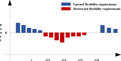
FIGURE 2. Flexibility requirement effect.

4.2 Analysis of system flexibility resource

Integrated energy system flexibility resources, including gas turbines, energy storage elements, and a large number of flexible loads that can participate in demand response, are gradually growing in size along with the rapid development of active distribution grids and have great dispatchable potential. These resources provide available flexibility for the system in terms of ensuring the reliability and economy of system operation, and fully exploiting the available flexibility capability of deploying such resources can allocate the optimal available flexibility for the system in multiple timescales. According to the different roles and operational characteristics of flexibility resources in the system, flexibility resources can be categorized into generation-type resources, storage-type resources, and load-type resources. Since these flexibility resources have different operating characteristics, the system can be supported with flexibility capabilities to respond to flexibility needs over multiple timescales. Based on the various types of characteristics of these resources, they can be categorized as short-time flexibility resources (less than 15 min), medium-time flexibility resources (15–60 min), and long-time flexibility resources (more than 1 h). First, short-term flexibility resources consist primarily of energy storage devices. Second, medium-time flexibility resources are mainly thermal power units. Long-time flexibility resources are mainly demand responses that respond to the system on a long timescale, and because of the delayed nature of gas and heat grids relative to the grid, they are categorized as resources that can provide flexibility to the system through demand responses on a long timescale.

Thermal units are more flexible and typically participate in short- and medium-timescale flexibility regulation, where the size of their flexibility resources is constrained by their upward and downward creep rates and their maximum and minimum operating outputs:

$\left\{\begin{array}{l}{F}_{G,+}=\min \left\{P_{G,\max }-P_{G,0},\Delta t\times r_{m,+}\right\}\\ F_{G,-}=\min \left\{P_{G,0}-P_{G,\min },\Delta t\times r_{m,-}\right\}\end{array}\right..(27)$

As a flexible power source that can be adjusted quickly, energy storage devices have different application scenarios depending on the energy storage technology and the size of the energy storage components.

$\left\{\begin{array}{l}{F}_{\text{soc},+}=\min \left\{P_{\text{soc}+,\max },\frac{S_t-S_{\min }}{\delta }\right\}\\ F_{\text{soc},-}=\min \left\{P_{\text{soc}-,\max },\frac{S_{\max }-S_t}{\delta }\right\}\end{array}\right..(28)$

Demand response controllable loads, according to their own load conditions and willingness to use electricity, take the initiative to assume a portion of the power dispatch responsibility, which is also one of the important ways to improve the flexibility of system dispatch. The size of its regulation resources is mainly determined by the load size of the demand-side response implementation organization and its own maximum output change restrictions.

$\left\{\begin{array}{l}{F}_{L,+}=\min \left\{P_{L,0},\Delta P_{L,-,\max }\right\}\\ F_{L,-}=\min \left\{P_{L,\max }-P_{L,0},\Delta P_{L,+,\max }\right\}\end{array}\right..(29)$

We calculate the flexibility available to the system at each timescale by using the flexibility requirements derived above and the flexibility support available to the system at multiple timescales.

$\Delta P_{\mathrm{f}}=P_g-P_l,(30)$

where P_g denotes the flexibility supply capacity of the system at each timescale and P_l denotes the flexibility demand situation of the system at each timescale.

In turn, statistics on the under-flexibility climb segments where flexibility resources are lower than flexibility needs are obtained to get the under-flexibility probability.

$P_{lack}=\frac{n}{N},(31)$

where n is the number of under-flexible climbing segments and N is the total number of climbing segments in the system.

Then, we calculate the flexibility deficit sample expectation by counting the flexibility deficit in the flexibility deficit climb segment to reflect the severity of the system flexibility gap.

$E_{\text{lack}}={\displaystyle \sum _{i=1}^n}\Delta F_{\text{lack},i}{P}_{\text{lack},i},(32)$

$\Delta F_{\text{lack},i}=\left\{\mid \Delta F_{\text{flex},i}‖\Delta F_{\text{flex},i}<0\right\},(33)$

where ∆F_lack,i is the size of the flexibility deficit in the i climbing segment.

In order to intuitively reflect the overall degree of flexibility of the system, on the basis of the above indicators, the flexibility indicators at each scale are weighted and summed to form the scale-weighted flexibility indicator F_sys. The weights of the scale indicators are determined by the decision maker, which can effectively reflect the impact of drastic fluctuations on the overall flexibility of the system.

$\left\{\begin{array}{l}{\mathbf{F}}_{\text{sys}}=\left\{{\overline{P}}_{\text{lack}},{\overline{E}}_{\text{lack}}\right\}\\ {\overline{E}}_{\text{lack}}={\displaystyle \sum ^k}{\omega }_i{E}_{\text{lack},i}\\ {\overline{P}}_{\text{lack}}={\displaystyle \sum _{i=1}^{\kappa }}{\omega }_i{P}_{\text{lack},i}\end{array}\right.,(34)$

where P_lack and E_lack are the scale-weighted under-flexibility probability and under-flexibility expectation that synthesize the under-flexibility k scales, respectively, and w_i is the assigned weight for scale i.

To summarize the above, the complete process for the assessment of available flexibility at multiple timescales for an integrated energy system is shown in Figure 3. The process is as follows:

1) The prediction curve is derived and compared with the actual system operating curve, and the upward and downward flexibility requirements of the system are calculated and decomposed.

2) Multi-timescale classification based on the analysis of the operational characteristics of each flexibility resource of the system and division are carried out to obtain the upward/downward flexibility supply capacity provided by the resource for the system under each timescale.

3) We solve for the available flexibility capacity of the system at each timescale by analyzing flexibility resources and requirements.

4) The upward/downward inflexibility probability and the inflexibility expectation metrics are calculated and weighed to obtain a composite metric for assessing the flexibility available to the system.

FIGURE 3

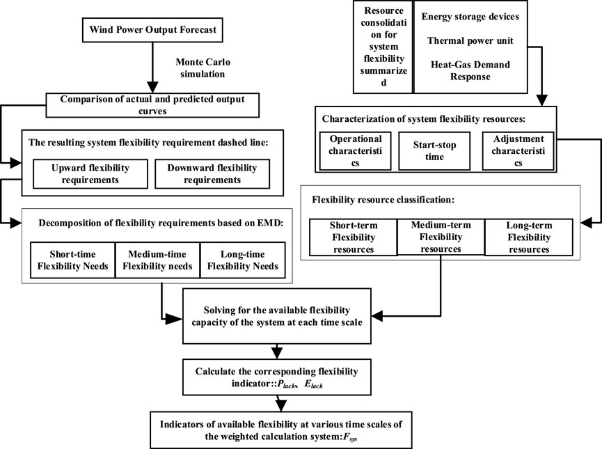
FIGURE 3. Flowchart for assessing available flexibility on multiple timescales.

5 Example analysis

In this paper, an integrated energy system consisting of an IEEE 39-node transmission system, a 20-node natural gas system, and a 6-node thermal system is solved and operationally analyzed by the YALMIP solver in MATLAB. In this case, the gas network is connected to the 33 nodes of the grid through a P2G device. The heat network is connected to 30 nodes of the grid through CHP units. The gas network is connected to 1 node of the heat network through a CHP unit. The specific system structure is shown in Figure 4.

FIGURE 4

FIGURE 4. Integrated energy system network node diagram.

5.1 Analysis of practical examples of integrated energy systems

This section evaluates the system target flexibility based on historical actual output data of wind power and load for an integrated energy system with intraday multi-scale flexibility. The total installed capacity of the system is 2,670 MW, the proportion of wind power installed is 15%, the maximum load is 1,974.48 MW, and the peak and valley difference of the maximum load in a day is 1,228.92 MW, respectively. The total capacity of the energy storage equipment in the system is 300 MWh, and the upper and lower limit of the single charging and discharging power is 100 MW; in addition, the specific system equipment parameters are shown in Table 1.

TABLE 1

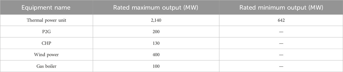
TABLE 1. Integrated energy system equipment parameter table.

Based on the historical wind power output data, the Monte Carlo simulation algorithm predicts the wind power output in the system and obtains the wind power output prediction curve in 24 h under a typical day. At the same time, a 15-min unit combination of the load-out curve of the electricity–gas–heat integrated energy system under a typical day is carried out to obtain the unit output under the corresponding output mode, as shown in Figures 5, 6. Among them, Figure 5 shows the actual output of each unit, the upper left figure shows the actual output of the system turbines, the upper right figure shows the actual output of the system CHP units, the lower left figure shows the actual output of the thermal units in the system, and the lower right figure shows the charging and discharging power of the system energy storage devices. Figure 6 shows the 24 h load profile of the system as well as the wind power forecast and actual output profile.

FIGURE 5

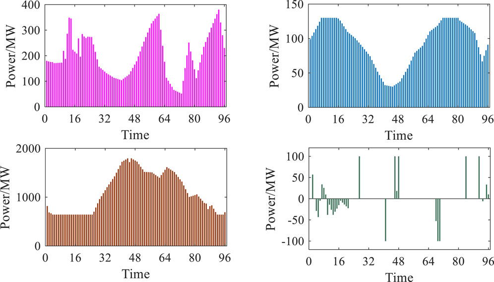
FIGURE 5. Chart of the output of each unit of the system.

FIGURE 6

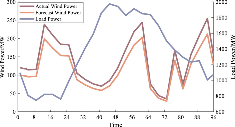
FIGURE 6. System wind power forecasts, actual output, and load profiles.

The EMD-based multi-timescale decomposition algorithm decomposes the target flexibility demand curve into three kinds of fluctuation components, namely, high-frequency (<15 min fluctuation), mid-frequency (15 min∼1 h fluctuation), and low-frequency (>1 h fluctuation), and then performs the waveform identification of the components in each scale to find the corresponding flexibility demand. Decomposing the system flexibility requirement curve under a typical day according to Eqs 25, 26, the result is obtained as shown in Figure 7. Where the vertical height of Figure 7 indicates the size of upward and downward flexibility demand, and the horizontal step indicates the flexibility demand fluctuation period. As can be seen from the figure, the fluctuations under different frequency bands are quite different, and the power fluctuations in high and medium frequency are mainly concentrated in the time periods of 2:00–6:00 and 18:00–22:00, and the power fluctuation is the largest in the time period of 2:00–6:00, which is consistent with the characteristics of the fluctuation of wind power output with the change of wind speed size. Influenced by load and wind power fluctuations, the maximum upward and downward flexibility demand for the low-frequency component occurs in the late-night and midday hours, respectively. Moreover, the distribution of flexibility demand is different in different flexibility directions, reflecting the directionality of flexibility fluctuations.

FIGURE 7

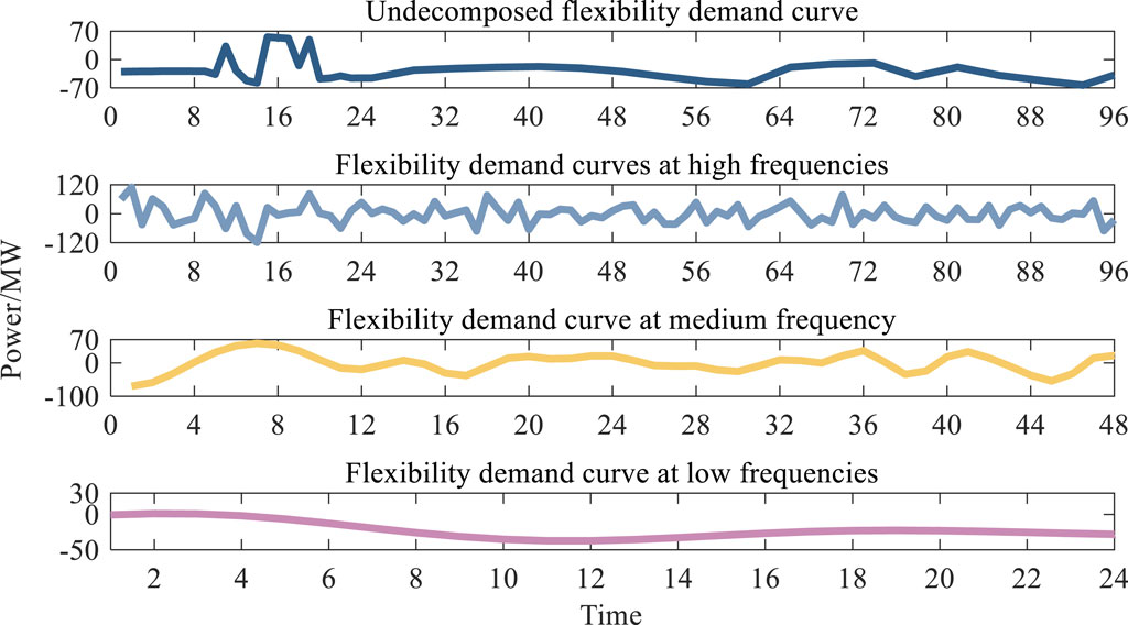
FIGURE 7. Decomposition of flexibility requirements for multi-timescale systems.

Based on the operating status, output regulation characteristics and fluctuation period of each type of flexibility resources, the upward and downward flexibility supply under different time scales is calculated by Eqs 27–29 as shown in Figure 8. As can be seen from the figure, there is a clear difference in the size of the flexibility resources on the high-, medium-, and low-frequency components. In addition, the flexibility resources in different directions have different distributions. According to the long-time flexibility curves, it can be seen that the flexibility supply capacities of the system at long timescales are all negative, which is due to the fact that the flexibility demands of the system at long timescales are all downward flexibility demands, which also reflects the influence of the difference in the upward and downward regulating capacity of the controllable units on the flexibility resources of the system and further illustrates the necessity of the directional characteristics in the flexibility assessment.

FIGURE 8

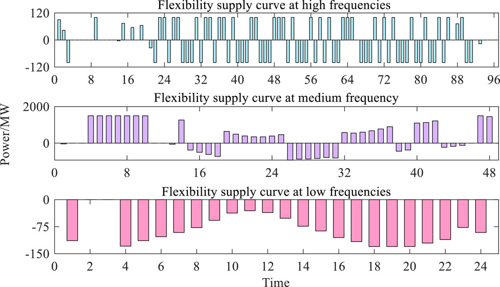
FIGURE 8. Map of the supply of flexibility in multi-timescale systems.

As shown in Figure 9, calculating the flexibility supply and demand at each time scale through Eq. 30 yields the available flexibility capacity of the system at multiple time scales. The bars above the x-axis represent the flexibility of the system that is readily available for deployment at that moment in time, and the bars below the x-axis represent the lack of flexibility of the system at that moment in time. From the figure, it can be seen that the system has high-frequency flexibility deficits under multi-timescale decomposition at 23:30–24:00, 0:30, and 2:45–3:15; on the one hand, this is due to the large variation of the wind speed in this time period, which leads to a larger error between the predicted wind power output and the actual output, so flexibility deficits are observed in this time period. On the other hand, the supply of high-frequency flexibility mainly relies on the energy storage device in the system, but the energy storage device is unable to perform charging and discharging operations at the same time, so it is unable to provide the flexibility required by the system in a timely manner, resulting in a shortage of flexibility.

FIGURE 9

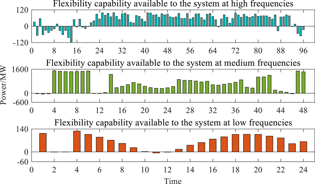
FIGURE 9. Map of available flexibility capacity for multi-timescale systems.

The proposed flexibility evaluation index system is utilized to assess the available flexibility capacity of the system under multiple timescales. By counting the number of flexibility deficit time periods and the size of flexibility deficit of the system under each timescale, the system’s flexibility deficit probability and flexibility deficit expectation index can be calculated according to Eqs 31, 32. Further weighting of the system flexibility metrics at each time scale through Eqs 33, 34 yields a composite flexibility rating metric. It should be noted that the weights of each timescale of the system are selected according to the needs of the decision maker, and if the decision maker pays more attention to the flexibility at a certain timescale, the weights of that timescale can be increased. In this paper, the weights are set to 40% for the long timescale, 40% for the medium timescale, and 20% for the short timescale, and the results of the system flexibility assessment are shown in Table 2.

TABLE 2

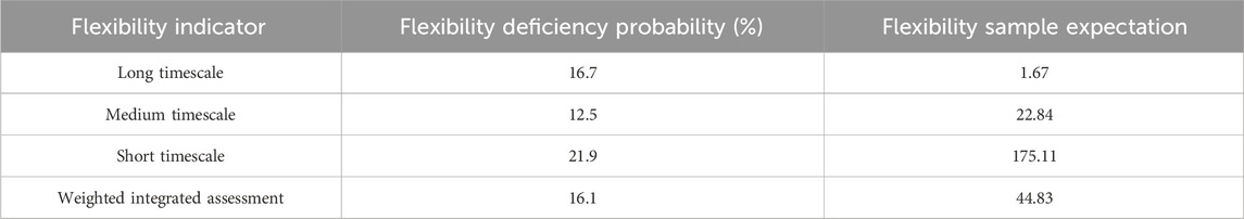
TABLE 2. Table of the results of the assessment of the system’s available flexibility capabilities.

From Table 2, it can be seen that comparing the flexibility assessment results under each scale horizontally, in this example system with only 15% of wind power access, the flexibility demand under high- and medium-frequency fluctuations is smaller, the probability of insufficient flexibility is lower, and the expectation of insufficient flexibility is smaller compared with low-frequency fluctuations when the overall flexibility of the system is more affected by low-frequency fluctuations. Thus, it suffers from less flexibility on low-frequency fluctuations.

5.2 Analysis of the impact of proportions of wind power installations on system flexibility assessment

In order to study the flexibility of the power system under large-scale wind power grid integration, this section sets up the analysis scenarios with 10% and 20% of wind power installed in Section 4.1, respectively, on the basis of varying the proportion of wind power installed, and compares them with the scenario with 15% of wind power installed in Section 4.1. By calculating the supply and demand for flexibility at each time scale, it is possible to obtain the supply and demand for flexibility at multiple time scales for wind power systems with different percentages of installed wind power. The available flexibility capacity of the system at different wind power installation ratios can be obtained by calculating the flexibility supply and demand at each timescale. The available flexibility capacity of the system at 10% wind power installation ratio is shown in Figure 10, the flexibility capacity of the system at 20% wind power installation ratio is shown in Figure 11, and the flexibility capacity of the system at 15% wind power installation ratio can be seen in Figure 9 in Section 4.1. Tables 3, 4 show the evaluation metrics for each timescale of the system at 10% installed base and 20% installed base, respectively.

FIGURE 10

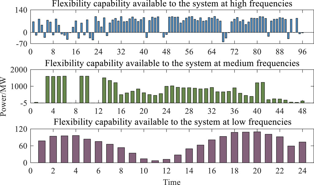
FIGURE 10. Flexibility capacity map of system availability at 10% installed capacity share.

FIGURE 11

FIGURE 11. Flexibility capacity map of system availability at 20% installed capacity share.

TABLE 3

TABLE 3. Table of the results of the assessment of the system’s available flexibility capacity at 10% of installed capacity.

TABLE 4

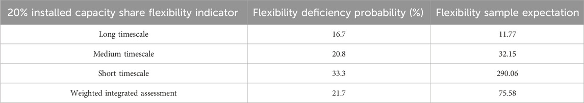
TABLE 4. Table of the results of the assessment of the system’s available flexibility capacity at 20% of installed capacity.

From Figures 10, 11, it can be seen that the available flexibility capacity of the system at the mid-frequency under the multi-timescale decomposition is much higher than that at the high and low frequencies, which is due to the fact that the resources supplying flexibility to the system at the mid-frequency are thermal units, which have a larger standby capacity and faster ramp-up to satisfy the system’s larger flexibility shortfalls as well as to respond to the system’s flexibility needs quickly so that the system’s available flexibility is larger at this frequency. On the other hand, the low-frequency available flexibility capacity under the multi-timescale decomposition is in the scarcity phase at 11–12 o’clock. Since the low-frequency demand of the total system at long timescales relies mainly on the demand response supply of the two systems, heat–gas, through coupled elements, at this point in time, both the P2G and CHP units are almost at maximum output and the system needs upward flexibility supply, so the available flexibility capacity of the system at this point in time is smaller.

As can be seen from Tables 2–4, the weighted probability of insufficient flexibility of the system increases significantly with the increase in the proportion of new energy access, indicating that access to new energy has a large impact on the flexibility of the system in all different directions. In Table 3, the long-timescale indicators under the scenario of 10% installed wind power are all 0. This is due to the smaller installed wind power proportions under this scenario and, thus, the smaller system flexibility demand caused by the wind power prediction error, and the system flexibility supply capacity under the longer timescale can fully satisfy the demand, and therefore, there is no flexibility shortage. On different fluctuation scales, the quantity source access in the large-scale new energy under-flexibility climb segment has a significant impact on system flexibility under medium- and high-frequency fluctuations and a lower impact on system flexibility under low frequency. This is because the new energy output represented by wind power has stronger fluctuation characteristics at medium and short timescales, and its large-scale grid connection has more obvious needs for the growth of system flexibility demand at medium and short timescales. Under low-frequency fluctuations, the change in downward flexibility is smoother compared to upward flexibility because of the complementary nature of wind power output on long timescales, and the access to a high proportion of new energy sources has a limited impact on the downward flexibility of the system on long timescales.

6 Conclusion

This paper focuses on the flexibility sufficiency of integrated energy systems at multiple timescales and proposes an integrated energy system flexibility assessment index and its calculation method based on EMD that effectively differentiates the flexibility needs at multiple timescales. The validity of the assessment methodology of this paper is verified using the actual operation of a real integrated energy system on a typical day as an example. The effects of different installed wind power capacities and different timescales on the results of system flexibility assessment are compared. The main conclusions are as follows: first, due to the different fluctuation characteristics of wind power output on various timescales, a high proportion of new energy generation has different impacts on the flexibility requirements of the system on different timescales; second, the EMD-based multi-scale decomposition algorithm can accurately derive independent multi-scale components in the scaling of flexibility, which is helpful for determining the flexibility demand under a specific fluctuation cycle, and further calculating the available flexibility capacity of the system, which is helpful for the operators to make scheduling allocations; and last, analyzing the available flexibility of the integrated energy system under different wind power installation ratios, wind power output has complementary characteristics on long timescales, and a high proportion of new energy access has a limited impact on the downward flexibility of the system on long timescales.

Data availability statement

The original contributions presented in the study are included in the article/Supplementary Material; further inquiries can be directed to the corresponding author.

Author contributions

SZ: conceptualization, supervision, and writing–review and editing. YZ: methodology, validation, and writing–original draft. SL: data curation, formal analysis, and writing–review and editing.

Funding

The authors declare that financial support was received for the research, authorship, and/or publication of this article. This work was supported by the Doctoral Research Initiation Fund of Northeast Electric Power University, and the project number is BSJXM-2022201.

Acknowledgments

The authors would like to thank the Northeast Electric Power University for its support in this work and all the people who contributed to this article.

Conflict of interest

The authors declare that the research was conducted in the absence of any commercial or financial relationships that could be construed as a potential conflict of interest.

Publisher’s note

All claims expressed in this article are solely those of the authors and do not necessarily represent those of their affiliated organizations, or those of the publisher, the editors, and the reviewers. Any product that may be evaluated in this article, or claim that may be made by its manufacturer, is not guaranteed or endorsed by the publisher.

References

Abdel-Ouahab, B., and Jean-Christophe, C. (2007). EMD-based signal filtering. IEEE Trans. Instrum. Meas. 56 (06), 2196–2202. doi:10.1109/tim.2007.907967

CrossRef Full Text | Google Scholar

Alireza, R., Gevork, B. G., Hamid Reza, B., and Roya, A. (2024). Aggregator index for 24-hour energy flexibility evaluation in an ADN including PHEVs. IEEE Access 12, 16105–16116. doi:10.1109/access.2024.3353136

CrossRef Full Text | Google Scholar

Fugui, D., Zihang, M., Laihao, C., and Xiaofeng, W. (2023). A multi-timescale optimal operation strategy for an integrated energy system considering integrated demand response and equipment response time. J. Renew. Sustain. Energy 15 (44). doi:10.1063/5.0159626

CrossRef Full Text | Google Scholar

Jia, S., Hsiao Dong, C., and Yuan, Z. (2021). Toward quantification of flexibility for an electricity-heat integrated energy system: secure operation region approach. IET Energy Syst. Integr. 3 (24), 142–157. doi:10.1049/esi2.12009

CrossRef Full Text | Google Scholar

Jiang, X., Li, Q., Yang, Y., Zhang, L. t., Liu, X. j., and Ning, N. (2022). Optimization of the operation plan taking into account the flexible resource scheduling of the integrated energy system. Energy Rep. 8, 1752–1762. doi:10.1016/j.egyr.2022.02.211

CrossRef Full Text | Google Scholar

Jiangxuan, W., Zhi, W., Yating, Z., Qirun, S., and Fujue, W. (2023). A robust flexibility evaluation method for distributed multi-energy microgrid in supporting power distribution system. Front. Energy Res. 10 (46). doi:10.3389/fenrg.2022.1021627

CrossRef Full Text | Google Scholar

Jiaying, C., Hao, L., Wei, H., Zhongbo, L., Wei, Z., Yi, Z., et al. (2020). A study on urban heating system flexibility: modeling and evaluation. J. Energy Resour. Technol. 142 (24). doi:10.1115/1.4045542

CrossRef Full Text | Google Scholar

Lusha, W., Jonghwan, K., Noel, S., and Zhi, Z. (2022). Evaluation of aggregated EV flexibility with TSO-DSO coordination. IEEE Trans. Sustain. Energy 13 (4), 2304–2315. doi:10.1109/tste.2022.3190199

CrossRef Full Text | Google Scholar

Qin, W., and Bri-Mathias, H. (2017). Enhancing power system operational flexibility with flexible ramping products: a review. IEEE Trans. Industrial Inf. 13 (116), 1652–1664. doi:10.1109/tii.2016.2637879

CrossRef Full Text | Google Scholar

Wenkai, D., Zhigang, L., Liangce, H., Jiangfeng, Z., and Tao, M. (2023). Optimal expansion planning model for integrated energy system considering integrated demand response and bidirectional energy exchange. CSEE J. Power Energy Syst. 9 (04), 1449–1459.

Google Scholar

Xiaolin, G., Xiaohe, Z., Yang, F., Yisheng, X., and Lingling, H. (2022). Optimization of reserve with different time scales for wind-thermal power optimal scheduling considering dynamic deloading of wind turbines. IEEE Trans. Sustain. Energy 13 (36), 2041–2050. doi:10.1109/tste.2022.3179635

CrossRef Full Text | Google Scholar

Xiaoou, L. (2020). Research on flexibility evaluation method of distribution system based on renewable energy and electric vehicles. IEEE Access 8, 109249–109265. doi:10.1109/access.2020.3000685

CrossRef Full Text | Google Scholar

Yewei, C., Jianjun, S., Xiaoming, Z., Yanhong, Y., and Feng, X. (2021). A novel node flexibility evaluation method of active distribution network for SNOP integration. IEEE J. Emerg. Sel. Top. Circuits Syst. 11 (1), 188–189.

Google Scholar

Ying, W., Kaifeng, Z., and Kaiping, Q. (2023). Segmented real-time dispatch model and stochastic robust optimization for power-gas integrated systems with wind power uncertainty. J. Mod. Power Syst. Clean Energy 111 (05), 1480–1493.

Google Scholar

Yuan, Z., Jiangjiang, W., Fuxiang, D., Yanbo, Q., Zherui, M., Yanpeng, M., et al. (2021). Novel flexibility evaluation of hybrid combined cooling, heating and power system with an improved operation strategy. Appl. Energy 300 (48), 117358. doi:10.1016/j.apenergy.2021.117358

CrossRef Full Text | Google Scholar

Yue, Q., Sunyang, Z., Wei, G., Shixing, D., Gaoyan, H., Kang, Z., et al. (2022). Multi-stage flexible planning of regional electricity-HCNG-integrated energy system considering gas pipeline retrofit and expansion. IET Renew. Power Gener. 16 (52), 3339–3367. doi:10.1049/rpg2.12586

CrossRef Full Text | Google Scholar

Yufei, Z., Chengfu, W., Zhenwei, Z., and Huacan, L. (2021). Flexibility evaluation method of power system considering the impact of multi-energy coupling. IEEE Trans. Industry Appl. 57 (6), 5687–5697. doi:10.1109/tia.2021.3110458

CrossRef Full Text | Google Scholar

Yuxiao, Q., Pei, L., and Zheng, L. (2021). Multi-timescale hierarchical scheduling of an integrated energy system considering system inertia. Renew. Sustain. Energy Rev. 169 (70).

Google Scholar

Zening, L., Su, S., Xiaolong, J., Mingchao, X., Qifang, C., and Koji, Y. (2021). Stochastic and distributed optimal energy management of active distribution network with integrated office buildings. CSEE J. Power Energy Syst., 1–12.

Google Scholar