Channel prediction method based on the data-driving for distribution automation main station

A data-driven channel prediction method for distribution automation master is proposed to address the poor quality of communication network and communication system transmission problems in distribution network communication. In this paper, an adaptive broad learning network (ABLN) consisting of a standard broad learning network and a hybrid learning network is introduced to predict the channel state information of the communication system. Among them, the hybrid learning network is used to solve the ill-conditioned solution problem when estimating the output weight matrix of the standard broad learning network. Therefore, the ABLN produces sparse output weight matrices and provides excellent prediction performance. In the simulation analysis, the outdoor and indoor scenes are considered based on OFDM system. The prediction performance of ABLN is subsequently evaluated in one step prediction and multistep prediction. The results show that for the prediction performance is concerned, the maximum improvement of ABLN is about 96.49% as compared to other evaluation models, indicating that the CSI is effectively predicted by the ABLN to support the adaptive transmission of the main station of the distribution automation and to satisfy the quality of the communication network of the distribution network.

1 Introduction

Currently, the distribution automation main station (DAMS) tends to huge network size, wide distribution, harsh environment, and frequent changes of distribution sites (Gu, 2017). The distribution communication network, as the nervous system of distribution network automation, is bound to meet the high-quality communication needs. Therefore, high-quality distribution network communication system is the foundation of the smart distribution network construction. The distribution network automation construction presents many challenges to the wireless communication system (Pan L et al., 2023). Generally speaking, the receiver of wireless communication system needs to estimate the channel state information (CSI) of transmission environment through channel estimation technique, and feedback the CSI to the transmitter. However, in fast time-varying communication environments, the CSI tends to be outdated, which degrades the adaptive transmission performance. Therefore, the channel prediction based on the outdated CSI is important to support the adaptive transmission performance of wireless communication systems such as power IoT (by Flam et al., 2006).

Currently, channel prediction methods can be classified into three categories, i.e., linear prediction methods parameter class prediction methods and nonlinear prediction methods (Sarankumar R et al., 2016) Among them, linear prediction methods are mainly used to predict the next channel state information sample by linearly weighting the sum of several CSI samples in the past by linear fitting. Currently, channel prediction methods can be classified into three categories,i.e., linear prediction methods parameter class prediction methods and nonlinear prediction methods. Among them, linear prediction methods are mainly used to predict the value of the next channel state information sampling point by linearly fitting the past several channel state information sampling points, i.e., by linearly weighting the sum. Linear prediction methods include the auto-regression (AR), the recursive least squares (RLS) and the affine projection algorithm (APA) (Kapoor et al., 2018). The parameter prediction method mainly estimates those relevant parameters of transmission delay, such as the power, the delay and the Doppler shift. In addition, errors in the estimated channel statistical characteristics and parameters reduce the accuracy of the channel prediction, so the errors in the parameter class prediction need to be reduced in order to improve the performance of adaptive transmission techniques for wireless communication systems. Scholars have developed relevant studies on parameter class channel prediction methods. Such as, Niu G Q et al. (2014) and Yang et al. (2021) proposed a new predictor that utilizes the powerful time series prediction capability of deep learning. The prediction result indicates that the deep learning can offer significant performance improvement compared with the traditional predictor. To overcome the problem caused by the nonlinearity of the transmission channel and inter-symbol interference caused by multipath effects, Tan and Wang, (2023) used deep learning networks to optimally research the channel equalization for the optical fiber communication networks, and constructed an optical fiber communication network channel model, and used deep learning networks to estimate the communication network channel loads and operational states. Trivedi and Kumar, (2018) used a scheduler based on a standardized SNR for selecting users for data transmission, the scheduler has higher data rate and long-range transmission capabilities without requiring much power or bandwidth. In addition, this paper presents a comparative assessment of the bit error rate (BER) performance of multi-user multiple input multiple output orthogonal frequency division multiplexing (MU-MIMO-OFDM) and MU-MIMO single-carrier frequency-division multiple access (MU-MIMO-SCFDMA) and investigates the impact of various factors, e.g., the CSI imperfections, network heterogeneity, and other factors on the communication transmission; Bai et al. (2020) proposed a prediction method based on the long short term memory (LSTM) network and developed an incremental learning scheme for dynamic scenarios, which makes the LSTM predictor run online; (Multiple-Input Multiple-Output, MIMO) system, based on the measured data of 2.35 GHz band in the road-wall scenario, C Xue et al. (2021) proposes a Convolutional Long Shore-Term Memory (CLSTM) and CNN combination of Conv- CLSTM channel prediction model for typical channel state information, Les K-factor, RMS delay extension and angle extension characteristics prediction. Son and Han, (2021) proposed the channel adaptive transmission (CAT), which uses the LSTM network for channel prediction and the prediction accuracy is over 97%, indicating that this algorithm can be effectively used for channel prediction. Jiang and Schotten, (2019) used the recurrent neural network (RNN) to construct a frequency domain channel predictor, which was integrated into the MIMO-OFDM system to improve the correctness of antenna selection. To avoid the degradation of communication quality, Ding and Hirose, (2013) proposed a high-accuracy time-varying channel prediction by using channel prediction with linear extrapolation and Varangian extrapolation of frequency-domain parameters, and by combining a multilayered complex neural network (CVNN) with a linear FM permutation method. The proposed CVNN-based predictive channel prediction accuracy is experimentally proved to be better than the traditional prediction methods (Ding and Hirose, 2014). Xu and Han, (2016) proposed a new model adaptive elastic echo state network (ESN), which adopts the adaptive elastic network algorithm to compute the unknown weights and combines the advantages of quadratic regularization and adaptive weighted lasso contraction to deal with the covariance problem.

In recent years, the deep learning has been successfully applied in many fields and played an important role in the field of the artificial intelligence field (Schofield et al., 2019). Wang et al. (2019b) proposed a hybrid deep learning method of Convolutional Neural Network (CNN) and LSTM to get the CSI of downlink channel based on the CSI of uplink channel in FDD system. By extending an LSTM for reconstructing CSI, Wang et al. (2019a) proposed a real-time CSI feedback framework applied to point-to-point massive MIMO. The application of deep learning in channel prediction successfully solves the problem of traditional manual methods that are overly dependent on channel-specific parameters and has a stronger ability to adapt to the environment. However, the deep learning methods still have some drawbacks. On the one hand, when facing the high-dimensional data, the deep learning is usually trained with a complex structure, which means that many model parameters need to be adjusted. On the other hand, when some new samples are added, the deep learning often needs to re-train the model, which is a quite time-consuming process. To address the issue above, Chen et al. (2018) developed the broad learning system (BLS). Unlike the deep learning model, the BLS only has two horizontally aligned hidden layers, i.e., the feature layer and the enhancement layer (Suganthan and Katuwal, 2021; Pao and Takefuji, 2021). In the training process of the BLS model, the input data are firstly generated into feature nodes by feature mapping, and then the feature nodes are enhanced into augmentation nodes by nonlinear changes. Finally, the output of the feature layer and the output of the enhancement layer are connected to generate the result of the final output layer. The output weights of the final output layer can be obtained quickly using the ridge regression algorithm without complex computation (Chen and Liu, 2018). In addition, BLS has an attractive advantage of the universal approximation property (Jin and Chen, 2018). In particular, the incremental learning algorithms of the BLS can be quickly reshaped without the need for complete retraining from scratch.

With these solid foundations mentioned above, a large amount of work on BLS has been reported. Kurtz, (1987) incorporated the and paradigm combination into the regular term of the elastic network into the BLS model thus obtaining ENBLS. ENBLS can benefit from the trend of both ridge regression and sparse solutions. However, there are still many drawbacks of the shallow structure, and the expressive ability is significantly weaker than that of the deep structure. For this reason, many scholars started to improve the standard BLS. Then, many more complex BLS appeared. Such as, Feng and Chen, (2020) integrated BLS with Takagi-Sugeno fuzzy system to generate the FBLS. In addition, to extend the applicability of BLS, Zhao et al. (2020) obtained Semi-Supervised BLS (SS-BLS) by introducing popular learning and thus extending BLS to semi-supervised learning. However, the SS-BLS requires all labelled training datasets, which limits the practicability in practical scenarios. Another structure of online semi-supervised BLS (Online SS-BLS, OSSBLS) was investigated in Pu and Li, (2020). In addition, Min et al. (2019) improved the BLS and obtained a Structured Manifold BLS (SM-BLS), which was used to predict the time-series. Zhang et al. (2020) also applied the BLS for the emotion recognition. Then, Liang, (2023) investigated a class of the distributed learning algorithms based on the BLS, which used a quantization strategy to reduce the number of bits per transmission and a communication review strategy to reduce the total number of transmissions and minimize the communication cost (Huong et al., 2023).

To meet the demand of the information transmission quality of the DAMS and solve the problem that the expired CSI reduces the adaptive transmission performance of wireless communication system, this paper proposes a channel prediction method for ADSM based on the ABLN, including the standard BLN and the hybrid regularization network. Thereinto, the ill-conditioned solution of the output weight matrix of the former is mainly solved by the latter. The hybrid regularization network contains two layers, the first layer is an adaptive weight factor generation network based on regularization, and the second layer is the output weight matrix estimation network based on the elastic network. The hybrid regularization network has the oracle property, which can effectively solve the output weight ill-conditioned solution problem of the BLN. Thus, the ABLN can provide well channel prediction performance.

2 Revelant theory

2.1 Channel estimation for OFDM systems

The channel prediction is an important technique to support the adaptive transmission of power IoT communication systems such as distribution network automation master stations. In this paper, it is assumed that the SCI changes slowly or steadily in a frame time, so the channel estimation process can be described as follows. Let $s_i\left(n\right)$ denote the $n$-th sample of the $i$-th complex-valued baseband time-domain transmission signal, then $s_i\left(n\right)$ can be expressed as

$s_i\left(n\right)={\displaystyle \sum _{l=0}^{L-1}}{\mathit{S}}_i\left(l\right){\mathrm{e}}^{\mathrm{j}2\pi nl/L}(1)$

where ${\mathit{S}}_i\left(l\right)$ denotes the frequency-domain transmit signal on the lth subcarrier of the $i$-th pilot OFDM symbol, $\mathrm{l}=0,1,2,\dots \dots ,L-1,L$ is the total number of subcarriers in each OFDM symbol. When the transmitting antenna sends out the transmit signal, the transmit signal reaches the receiving antenna through the time domain channel. Therefore, the receiving end estimates the target CSI by analyzing the received signal. Currently, the two commonly used channel estimation methods are least squares (LS) method and the minimum mean square error (MMSE) method. The process of the channel estimation by LS method is [29]

$Y_i\left(m\right)=\frac{E_i\left(m\right)}{S_i\left(m\right)}+R_i\left(m\right)=Y_i\left(m\right)+R_i\left(m\right)(2)$

where $Y_i\left(m\right)$, $Y_i\left(m\right)$, $E_i\left(m\right)$ and $R_i\left(m\right)$ are the estimated CSI of the $i$-th subcarrier of the OFDM symbol, the ideal CSI, the received symbols, and the corresponding noise for the first subcarrier of the OFDM symbol at the first pilot subcarrier, respectively. $R_i\left(m\right)$ is modelled as the additive white gaussian noise (AWGN) with mean 0 and variance ${\sigma }_z^2$.

2.2 The broad learning system (BLS)

As shown in Figure 1, the BLS is used as an alternative to deep network structure. The input data is mapped to the mapping features and the enhancement features. The output layer connects the feature and enhancement layers. The data is transformed using a linear mapping function connecting the input weight matrices to obtain the set of mapped features. The ${\mathit{Z}}_i$ is the mapped feature, which is obtained by linear mapping and activation function, i.e.

${\mathit{Z}}_i={\phi }_i\left({\mathit{X}\mathit{V}}_{ei}+{\alpha }_{ei}\right),i=1,2,\dots ,n(3)$

where $X\in R^{a\times b}$ denotes the input sample data for model training, where a is the sample number and b is the dimension. The ${\phi }_i$ is the activation function of the feature node, ${\alpha }_{ei}$ denotes the input layer to the mapping feature layer. The mapping feature group is denoted as

${\mathit{Z}}^m=\left[{\mathit{Z}}_1,{\mathit{Z}}_2,{\mathit{Z}}_3,\dots ,{\mathit{Z}}_m\right](4)$

Figure 1

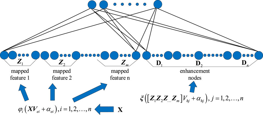
Figure 1. The typical network structure of BLS.

The enhancement nodes are obtained from the mapped nodes by the nonlinear mapping and the activation function transformation. $Y_j$ is the jth set of augmented nodes, which is

$Y_j={\mathit{\xi }}_j\left({\mathit{Z}}^m{V}_{hj}+{\alpha }_{hj}\right),j=1,2,\dots ,n(5)$

where ${\mathit{\xi }}_j$ is the activation function of the enhancement node; $V_{hj}$ denotes the random connection weight matrix of the $j$-th group of mapped feature nodes to the layer of enhancement nodes; ${\alpha }_{hj}$ is the bias matrix of the $j$-th group, and the group of enhancement nodes obtained by the n-transform is denoted by

${\mathbf{D}}^n=\left[{\mathbf{D}}_1,{\mathbf{D}}_2,{\mathbf{D}}_3,\dots ,{\mathbf{D}}_n\right](6)$

Then, the outputs of the feature nodes and enhancement nodes are combined, i.e., $F=\left[Z_m\left|D_n\right.\right]$. The weighted mapping of F, forms the output of the network $\widehat{H}=FV$. The mapped feature nodes and enhancement nodes are used as inputs to the BLS and the feature vectors are solved. V denotes the weight matrix from the input layer to the output layer of the system, which is solved by solving the ridge regression, i.e.,

$\mathbf{V}={\left(\lambda \mathit{I}+{\mathbf{H}}^{\mathrm{T}}\mathbf{H}\right)}^{-1}{\mathit{F}\mathit{H}}^{\mathrm{T}}(7)$

where the H denotes the regularization factor and I denotes the unit matrix.

3 Channel predictionbased of adaptive BLS

3.1 ABLN

The hidden layer of a typical BLN often has a large number of neurons. After using Eq. 5 to estimate the BLS network’s output weight matrix, the estimated value is generally an ill-conditioned solution, which has a large amplitude. Therefore, the ill-conditioned solution problem of the output weight matrix is a problem that cannot be ignored in the training process of the BLN (Zhou, 2013). To improve the ABLN’s generalization capabilities throughout the learning process, this study proposes using a hybrid generalization network to estimate the output weight matrix. The initial layer of the hybrid generalization network looks like this:

$J_k=\arg \underset{{\widehat{Q}}_{:,i}}{\min }{\left\{{‖{\mathbf{Y}}_i-\mathbf{Z}{\mathbf{Q}}_{:,i}‖}_2^2+{\lambda }_1{‖{\mathbf{Q}}_{:,i}‖}_2^2+{\lambda }_{\raisebox{1ex}{$1$}\!\left/ \!\raisebox{-1ex}{$2$}\right.}{‖{\mathbf{Q}}_{:,i}‖}_{\frac{1}{2}}^{\frac{1}{2}}\right\}}_k(8)$

where i = 1,2,3, ., I, ${\mathbf{Y}}_i$ denotes the target output corresponding to the $i$-th step prediction, ${\mathbf{Q}}_{:,i}$ is the estimated value of the target output weight matrix corresponding to the $i$-th prediction. ${‖*‖}_2$ and ${‖*‖}_{\raisebox{1ex}{$1$}\!\left/ \!\raisebox{-1ex}{$2$}\right.}$ denote the l₂ norm and l_1/2 norm, respectively, and ${\lambda }_{\raisebox{1ex}{$1$}\!\left/ \!\raisebox{-1ex}{$2$}\right.}$ is the generalization coefficient of l_1/2 norm. Therefore, the first layer is further expressed as

$\begin{array}{l}{J}_k=\arg {\underset{{\widehat{Q}}_{:.i}}{\min }\left\{{‖{\mathbf{Y}}_i-\mathbf{Z}{\mathbf{Q}}_{:,i}‖}_2^2+{\lambda }_1{‖{\mathbf{Q}}_{:,i}‖}_2^2+{\lambda }_{\raisebox{1ex}{$1$}\!\left/ \!\raisebox{-1ex}{$2$}\right.}{‖{\mathbf{Q}}_{:,i}‖}_{\frac{1}{2}}^{\frac{1}{2}}\right\}}_k\\ =\arg \underset{{\widehat{Q}}_{:.i}}{\min }\left\{\begin{array}{l}{‖{\mathbf{Y}}_1-\mathbf{Z}{\mathbf{Q}}_{:,1}‖}_2^2+{\lambda }_1{‖{\mathbf{Q}}_{:,1}‖}_2^2+{\lambda }_{\raisebox{1ex}{$1$}\!\left/ \!\raisebox{-1ex}{$2$}\right.}{‖{\mathbf{Q}}_{:,1}‖}_{\frac{1}{2}}^{\frac{1}{2}}+\\ {‖{\mathbf{Y}}_2-\mathbf{Z}{\widehat{\mathbf{Q}}}_{:,2}‖}_2^2+{\lambda }_1{‖{\widehat{\mathbf{Q}}}_{:,2}‖}_2^2+{\lambda }_{\raisebox{1ex}{$1$}\!\left/ \!\raisebox{-1ex}{$2$}\right.}{‖{\widehat{\mathbf{Q}}}_{:,2}‖}_{\frac{1}{2}}^{\frac{1}{2}}+\\ ⋮\\ {‖{\mathbf{Y}}_I-\mathbf{Z}{\mathbf{Q}}_{:,I}‖}_2^2+{\lambda }_1{‖{\mathbf{Q}}_{:,I}‖}_2^2+{\lambda }_{\raisebox{1ex}{$1$}\!\left/ \!\raisebox{-1ex}{$2$}\right.}{‖{\mathbf{Q}}_{:,I}‖}_{\frac{1}{2}}^{\frac{1}{2}}\end{array}\right\}\end{array}(9)$

Therefore, the above Eq. 9 is equivalent to solve the following issue, i.e.,

$J_k=\arg \underset{{\widehat{Q}}_{:.i}}{\min }{\left\{{‖{\mathbf{Y}}_i-\mathbf{Z}{\mathbf{Q}}_{:,i}‖}_2^2+{\lambda }_1{‖{\mathbf{Q}}_{:,i}‖}_2^2+{\lambda }_{\raisebox{1ex}{$1$}\!\left/ \!\raisebox{-1ex}{$2$}\right.}{‖{\mathbf{Q}}_{:,i}‖}_{\frac{1}{2}}^{\frac{1}{2}}\right\}}_k(10)$

where $i=1,2,3,...,I$. Then, the above equation is rewritten as

$\begin{array}{l}{J}_k=\arg \underset{Q_{:,i}}{\min }{\left\{{‖{\mathbf{Y}}_i-\mathbf{Z}{\widehat{\mathbf{Q}}}_{:,i}‖}_2^2+{\lambda }_1{‖{\widehat{\mathbf{Q}}}_{:,i}‖}_2^2+{\lambda }_{\raisebox{1ex}{$1$}\!\left/ \!\raisebox{-1ex}{$2$}\right.}{‖{\mathbf{Q}}_{:,i}‖}_{\frac{1}{2}}^{\frac{1}{2}}\right\}}_k\\ =\arg \underset{Q_{:,i}}{\min }{\left\{\left(\begin{array}{l}{‖\left[\begin{array}{c}{\mathbf{Y}}_i\\ 0\end{array}\right]-{\left(1+{\lambda }_2\right)}^{-\raisebox{1ex}{$1$}\!\left/ \!\raisebox{-1ex}{$2$}\right.}\left(\begin{array}{c}\mathbf{Z}\\ \sqrt{{\lambda }_2}I\end{array}\right){\widehat{\mathbf{Q}}}_{:,i}‖}_2^2\\ +\frac{{\lambda }_2}{\sqrt{1+{\lambda }_{1/2}}}{‖{\mathbf{Q}}_{:,i}‖}_{\frac{1}{2}}^{\frac{1}{2}}\end{array}\right)\right\}}_k\\ =\arg \underset{Q_{:,i}}{\min }{\left\{‖{\widehat{\mathbf{Y}}}_i-\widehat{\mathbf{Z}}{{\widehat{\mathbf{Q}}}_{:,i}}^{\prime }‖+{\mathit{\lambda }}_b{‖{\mathbf{Q}}_{:,i}‖}_{\frac{1}{2}}^{\frac{1}{2}}\right\}}_k\end{array}(11)$

where

${\widehat{\mathbf{Y}}}_i=\left[\begin{array}{c}{\mathbf{Y}}_i\\ 0\end{array}\right](12)$

$\widehat{\mathbf{Z}}={\left(1+{\lambda }_2\right)}^{-\raisebox{1ex}{$1$}\!\left/ \!\raisebox{-1ex}{$2$}\right.}\left(\begin{array}{c}\mathbf{Z}\\ \sqrt{{\lambda }_2}I\end{array}\right)(13)$

${\mathit{\lambda }}_b=\frac{{\lambda }_2}{\sqrt{1+{\lambda }_{1/2}}}(14)$

Equation 11 is an optimization problem about l_1/2 norm. However, the l_1/2 norm is the non-convex and non-smooth, and some common optimization solution methods, i.e., the Newton’s method and simulated Newton’s method are difficult to solve the optimization Eq. 11. The coordinate descent method is utilized to solve Eq. 11 and its computation process is shown in Algorithm 2. Then the adaptive weighting factor ${\delta }_{:,i}$ for the first layer is

${\delta }_{:,i}={\left[\left|{\mathbf{Q}}_{:,i}\right|+\frac{1}{\left(M+L\right)}\right]}^{-\tau }(15)$

where $\tau \in {\mathbf{N}}_{+}$ is the adaptive adjustment factor. The second layer of the output weight matrix estimation network for the BLN is:

$J_k=\arg \underset{Q_{:,i}}{\min }{\left\{{\displaystyle \sum _{i=1}^I}\left(\begin{array}{l}{‖{\mathbf{Y}}_i-\mathbf{Z}{\mathbf{Q}}_{:,i}‖}_2^2+{\lambda }_1{‖{\mathbf{Q}}_{:,i}‖}_2^2+\\ {\lambda }_2{\displaystyle \sum _{j=1}^{M+L}}\left({\delta }_{j,i}{\mathbf{Q}}_{j,i}\right)\end{array}\right)\right\}}_k(16)$

where ${\mathbf{Q}}_{:,i}$ is the output weight matrix corresponding to the $i$-th prediction, ${\mathbf{Q}}_{j,i}$ denotes the jth element of the output weight matrix corresponding to the $i$-th step prediction, and ${\lambda }_1$ and ${\lambda }_2$ are the non-zero penalty coefficients, respectively. Eq. 16 can be further rewritten as

$\begin{array}{l}{J}_k=\arg \underset{Q_{:,i}}{\min }{\left\{{\displaystyle \sum _{i=1}^I}\left(\begin{array}{l}{‖{\mathbf{Y}}_i-\mathbf{Z}{\mathbf{Q}}_{:,i}‖}_2^2+{\lambda }_1{‖{\mathbf{Q}}_{:,i}‖}_2^2\\ +{\lambda }_2{\displaystyle \sum _{j=1}^{M+L}}\left({\delta }_{j,i}{\mathbf{Q}}_{j,i}\right)\end{array}\right)\right\}}_k\\ =\arg \underset{Q_{:,i}}{\min }\left\{\begin{array}{l}{‖{\mathbf{Y}}_1-\mathbf{Z}{\mathbf{Q}}_{:,1}‖}_2^2+{\lambda }_2{‖{\mathbf{Q}}_{:,1}‖}_2^2+{\lambda }_1{\displaystyle \sum _{j=1}^{M+L}}\left({\delta }_{j,1}{\mathbf{Q}}_{j,1}\right)\\ +{‖{\mathbf{Y}}_2-\mathbf{Z}{\mathbf{Q}}_{:,2}‖}_2^2+{\lambda }_2{‖{\mathbf{Q}}_{:,2}‖}_2^2+{\lambda }_1{\displaystyle \sum _{j=1}^{M+L}}\left({\delta }_{j,2}{\mathbf{Q}}_{j,2}\right)\\ ⋮\\ {‖{\mathbf{Y}}_I-\mathbf{Z}{\mathbf{Q}}_{:,I}‖}_2^2+{\lambda }_1{‖{\mathbf{Q}}_{:,I}‖}_2^2+{\lambda }_2{\displaystyle \sum _{j=1}^{M+L}}\left({\delta }_{j,i}{\mathbf{Q}}_{j,I}\right)\end{array}\right\}\end{array}(17)$

It can be shown that the loss function (17) of the second layer output weight matrix estimation network can also be converted into an I optimization problem with respect to the l2 norm and the adaptive weighting factors, i.e.,

$J_k=\arg \underset{Q_{:,i}}{\min }{\left\{{‖{\mathbf{Y}}_i-\mathbf{Z}{\mathbf{Q}}_{:,i}‖}_2^2+{\lambda }_1{‖{\mathbf{Q}}_{:,i}‖}_2^2+{\lambda }_2{\displaystyle \sum _{j=1}^{M+L}}\left({\delta }_{j,i}{\mathbf{Q}}_{j,i}\right)\right\}}_k(18)$

where $i=1,2,3,\dots ,I$. Eq. 17 can be further derived as:

$\begin{array}{l}{J}_k=\arg \underset{Q_{:,i}}{\min }{\left\{{‖{\mathbf{Y}}_i-\mathbf{Z}{\mathbf{Q}}_{:,i}‖}_2^2+{\lambda }_1{‖{\mathbf{Q}}_{:,i}‖}_2^2+{\lambda }_2{\displaystyle \sum _{j=1}^{M+L}}\left({\delta }_{j,i}{\mathbf{Q}}_{j,i}\right)\right\}}_k\\ =\arg \underset{Q_{:,i}}{\min }{\left\{\left(\begin{array}{l}{‖\left[\begin{array}{c}{\mathbf{Y}}_i\\ 0\end{array}\right]-{\left(1+{\lambda }_2\right)}^{-\raisebox{1ex}{$1$}\!\left/ \!\raisebox{-1ex}{$2$}\right.}\left(\begin{array}{c}\mathbf{Z}\\ \sqrt{{\lambda }_2}I\end{array}\right){\mathbf{Q}}_{:,i}‖}_2^2\\ +\frac{{\lambda }_2}{\sqrt{1+{\lambda }_2}}{\displaystyle \sum _{j=1}^{M+L}}\left({\delta }_{j,i}{\mathbf{Q}}_{j,i}\right)\end{array}\right)\right\}}_k\\ =\arg \underset{Q_{:,i}}{\min }{\left\{‖{\mathbf{Y}}_i^{\prime }-{\mathbf{Z}}^{\prime }{{\mathbf{Q}}_{:,i}}^{\prime }‖+{\mathit{\lambda }}_s{\displaystyle \sum _{j=1}^{\mathit{M}+\mathit{L}}}\left({\delta }_{j,i}{\mathbf{Q}}_{j,i}\right)\right\}}_k\end{array}(19)$

Where ${\mathbf{Y}}_i^{\prime }$, ${\mathbf{Z}}^{\prime }$, ${{\mathbf{Q}}_{:,i}}^{\prime }$ and ${\mathit{\lambda }}_s$ are defined as follows:

${\left.{\mathbf{Y}}_i^{\prime }=\left[\begin{array}{cc}{Y}_j& \mathbf{0}\end{array}\right.\right]}^{\mathrm{T}}(20)$

${\mathbf{Z}}^{\prime }={\left(1+{\lambda }_2\right)}^{-\frac{1}{2}}{\left[\begin{array}{cc}z& \sqrt{{\lambda }_2}I\end{array}\right]}^T(21)$

${{\mathbf{Q}}_{:,i}}^{\prime }=\sqrt{1+{\mathit{\lambda }}_2}{w}_i(22)$

${\lambda }_s=\frac{{\lambda }_1}{\sqrt{1+{\lambda }_2}}(23)$

where I is the unit matrix. It can be shown that Eq. 18 is an optimization problem with respect to the adaptive weighting factors. Further definition.

${\mathbf{Q}}_{j,i}^{″}={\delta }_{j,i}{\mathbf{Q}}_{j,i}^{\prime }(24)$

${\mathbf{Z}}^{″}=\frac{{\mathbf{Z}}^{\prime }}{{\delta }_{:,i}}(25)$

Eq. 19 can be further rewritten as:

$\begin{array}{l}{J}_k=\arg \underset{Q_{:,i}^{\prime }}{\min }{\left\{{‖{\mathit{Y}}_i^{\prime }-{\mathbf{Z}}^{\prime }{\mathbf{Q}}_{:,i}^{″}‖}_2^2+\mathit{\lambda }{\displaystyle \sum _{j=1}^{\mathit{M}+\mathit{L}}}\left({\mathbf{Q}}_{j:,i}^{″}\right)\right\}}_k\\ =\arg \underset{Q_{:,i}^{\prime }}{\min }{\left\{{‖{\mathit{Y}}_i^{\prime }-{\mathbf{Z}}^{\prime }{\mathbf{Q}}_{{:}^{\prime }i}^{″}‖}_2^2+\mathit{\lambda }‖{\mathbf{Q}}_{:,i}^{″}‖\right\}}_k\end{array}(26)$

Eq. 26 is an optimization problem with respect to the $L_1$-paradigm. Currently, some methods are available, such as the Newton’s method and the gradient descent method. All of the approaches, though, need the solution variables’ derivatives. In this study, we answer Eq. 27 using the minimal angle regression (MAR) approach, which avoids the derivatives of the variables. When ${\mathbf{Q}}_{:,i}^{″}$ is obtained, the output weight matrix ${\mathbf{Q}}_{:,i}$ corresponding to the ith step prediction is

${\mathbf{Q}}_{:,i}=\frac{{\mathbf{Q}}_{:,i}^{″}}{\left({\delta }_{:,i}\sqrt{1+{\lambda }_2}\right)}(27)$

Equation 27 is further modified as (Rodan, 2012):

${\mathbf{Q}}_{:,i}=\frac{\sqrt{1+{\lambda }_2}}{{\delta }_{:,i}}{\mathbf{Q}}_{:,i}^{″}(28)$

Therefore, the output weight matrix ${\mathbf{Q}}_{out}$ is

Algorithm 1. Calculation process of the ABLN.

Input: training output matrix $\mathbf{Y}$, training input matrix $\mathbf{Z}$, penalty coefficients ${\lambda }_1$, ${\lambda }_2$ and ${\lambda }_{1/2}$, adaptive factors $\tau$, maximum prediction step number $I$

Output: weight matrix ${\mathbf{Q}}_{out}$

Step 1: For $i=1,2,3,\dots ,I$

Step 2: Solve Eq. 8 to obtain ${\mathbf{Q}}_{:,i}$;

Step 3: Calculate the ${\delta }_{j,i}$ by Eq. 15;

Step 4: Calculate the modified ${\mathbf{Y}}_i^{\prime }$ by Eq. 20;

Step 5: Calculate the modified ${\mathbf{Z}}^{″}$ by Eq. 21;

Step 6: Solve Eq. 26 by the minimum angle regression method;

Step 7: Estimate by Eq. 28.

end

Step 8: Construct the output weight matrix ${\mathbf{Q}}_{out}$ by Eq. 29

Step 9: Output ${\mathbf{Q}}_{out}$;

Algorithm 2. Coordinate descent computation procedure.

Inputs: input: training output matrix $\mathbf{Y}$, training output matrix $\mathbf{Z}$, non-zero penalty coefficients ${\lambda }_{\raisebox{1ex}{$1$}\!\left/ \!\raisebox{-1ex}{$2$}\right.}$, empty matrix ${\mathbf{Q}}_{:,i}^0$

Output: ${\mathbf{Q}}_{:,i}$;

Step 1: ${\mathbf{Q}}_{:,i}={\mathbf{Q}}_{:,i}^0$;

Step 2: For $j=1,2,3,\dots ,L+M$;

Step 3: ${\mathbf{Q}}_{:,i}^0={\mathbf{Q}}_{:,i}$;

Step 4: Estimate ${\mathbf{Q}}_{:,i}$, $p=1,2,3,..,j$;

Step 5: Judge ${\displaystyle \sum _{j=1}^{M+L}}\left|{\mathbf{Q}}_{j,i}^0-{\mathbf{Q}}_{j,i}\right|\le \epsilon$. If no, then jump back to step 3; If yes, then jump to step 2.

End

$\left.{\mathbf{Q}}_{out}=\left[{\mathbf{Q}}_1,{\mathbf{Q}}_2,\cdots ,{\mathbf{Q}}_I\right.\right](29)$

The computational pseudo-code for the ABLN is shown in Algorithm 1 and the computational pseudo-code for the coordinate descent method is shown in Algorithm 2.

4 Simulation and discussion

These related parameters are part of the channel prediction approach for the DAMS based on ABLN that is looked at in this paper; they are shown in Table 1. Both the interior and outdoor scenarios are taken into consideration in order to assess how well ABLN performs.

1) The indoor scenario: Among the pertinent features are the maximum Doppler shift of 80 Hz and the total of six transmission routes; the delay and power are, respectively, (0, 120, 430, 860, 1030, 1470) ns and (0, −1.6, −0.8, −9, −9.4, −2.8) dB.

2) The outdoor scenario: The relevant parameters for the Nakagami-m channel scenario are as follows: The maximum Doppler shift is 20 Hz, and m is set to 5. Then, there are a total of four transmission lines, each having the following powers and de-lays: 0 dB and (0, 130, 230, 1180) ns, respectively.

Table 1

Table 1. Model parameter settings for the channel prediction method based on adaptive broad learning network.

This work also examines several of the current BLN-based methodologies, such as the fundamental BLN (Zhao and Lu, 2023), the lasso regularized BLN (LBLN) (Duan and Xu, 2022), the BLN with the ridge regularization (RBLN) (Wang, 2022) and the elastic network BLN (EBLN) (Ding and Xie, 2023). The following three performance metrics are considered in this paper.

1) The difference between the ideal and expected CSI is represented by the Root Mean Square Error, or RMSE. Thus, the prediction performance is evaluated in this paper using RMSE. Better predictive performance of the model is indicated by a reduced root mean square error.

2) The examined model’s ability to generate sparse output weight matrices is shown by its average sparsity. Again, a sparse output weight matrix demonstrates the significant improvement in the model’s memory use.

3) The average time spent is used to determine how complex the computation is during the output weight matrix estimation procedure. When the average time to estimate the output weight matrix is lower for a given model, we can conclude that the model has less computational complexity.

These three metrics are computed and examined in terms of one step and multi-step prediction in this section. The three measures are averaged over ten runs to remove randomness. The average sparsity for one step prediction is the mean number of non-zero elements in the projected output weight matrix after 10 iterations. The average sparsity in multi-step prediction is defined as the average rate of non-zero elements in the predicted output weight matrix from one step prediction to h-step prediction. Besides, in the simulation, the relevant parameter parameters of the ABLN include the neuron number of the feature layer 100, the neuron number 50, the input scaling factor 0.01 of the feature layer. Random generation is used to create both the input weight matrix and the internal weight matrix within the interval [-1, 1]. Each OFDM symbol has 60 subcarriers, as seen in Table 1, and 120 predictors might theoretically be used to complete the IDFT process. To keep things simple, the model utilized in this research is only evaluated using the CSI samples of the first subcarrier. The model is trained in ABLN using 5000 frames, and its performance is then assessed using the 1000 frames that follow.

4.1 Input dimensions of ABLN

The model’s input dimensions have an impact on the prediction performance. As a result, in two channel cases, the input dimensions of ABLN must be estimated. We present simulation results and a discussion of input dimensions in ABLN in this sub-section. Table 1 provides these regularization parameters. The x-axis of Figure 2, which shows the RMSE curves and non-zero weight curves of the predicted output weight matrices of both evaluation models in the two scenarios given, represents the input dimension of the ABLN, or the total CSI samples utilized to forecast the next CSI sample. The relationship between the RMSE and the input dimension p is thus shown by the red curve with a solid red circle, and the RMSE is represented by the left vertical axis. Similarly, the black curve labeled with black solid triangles represents the relationship between the number of non-zero components and the input dimension p, and the number of non-zero elements in the expected output weight matrix is displayed on the right vertical axis.

Figure 2

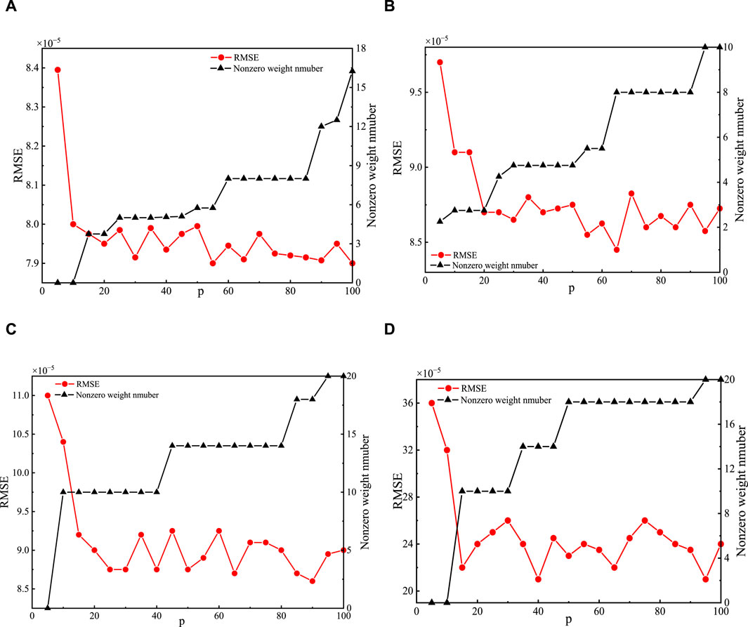
Figure 2. Non-zero weight curves and RMSE curves in ABLN with varying input dimensions: The actual and hypothetical components of the indoor scenario are shown in (A,B), respectively; The actual and imagined components of the outdoor landscape are shown in (C,D).

Generally, as the input dimension of the ABLN increases, the RMSE tends to decrease. Furthermore, when the input dimension increases, the projected output weight matrix’s non-zero members also grow. In Figure 2A, due to the increasing input dimensions, the RMSE curve of the real part of the CSI samples tends to stabilize in the indoor scenario, and the final RMSE is about 7.9e-4. Because of the increasing input dimensions, the redundancy information in Figure 2A raises the number of non-zero components of the projected output weight matrix. As a result, the lowering.

RMSE has a significant impact on the predicted output weight matrix’s sparsity. The primary ex-planation behind this is that as input dimensions grow, the ABLN model has access to more data and may perform better when making predictions. The number of non-zero items in the predicted output weight matrix rises as a result of the increased redundant information brought about by the larger input dimensions. Generally, the actual fraction of the CSI samples in the interior situation should have an input dimension of about 35. Subsequently, regarding the fictitious portion of the CSI samples in the indoor setting, the stabilized RMSE is about 8.8e-5, and the appropriate input dimension is about 35. Thus, in the indoor scenario, we set the input dimensions to 35 for both the imaginary portion of the CSI samples and the real values. Then the external situation Figure 2 display the non-zero weight curves and RMSE curves. The steady RMSEs of the real and imaginary sections of the CSI samples are, as can be shown from Figures 2C, D, approximately 9.2e-5 and 2.4e-4, respectively, just like in the indoor scene. Therefore, we also adjust the input dimensions of the real and imaginary sections of the CSI samples in the outdoor scene set to 35 to reduce the amount of non-zero weights in the estimated weight matrices.

4.2 One step prediction

Table 2 provides the regularization settings in ABLN for one step prediction. Moreover, the cost parameter c in the c-SVC, gamma in the kernel function, epsilon p in the SVM loss function, and 25, 0.001 and 2e-5 for the outside scenario are assigned the values 25, 0.006, and 2e-5. c, g and p for these evaluated model predictive performances are shown in Table 3. Figure 3 shows the ideal CSI curves, projected CSI curves, and error curves of the ABLN in the indoor scene and outdoor scenario for the real and imaginary halves of the CSI sample. The distribution range of these assessment models’ estimated output weight matrices is displayed in Figure 4.

Table 2

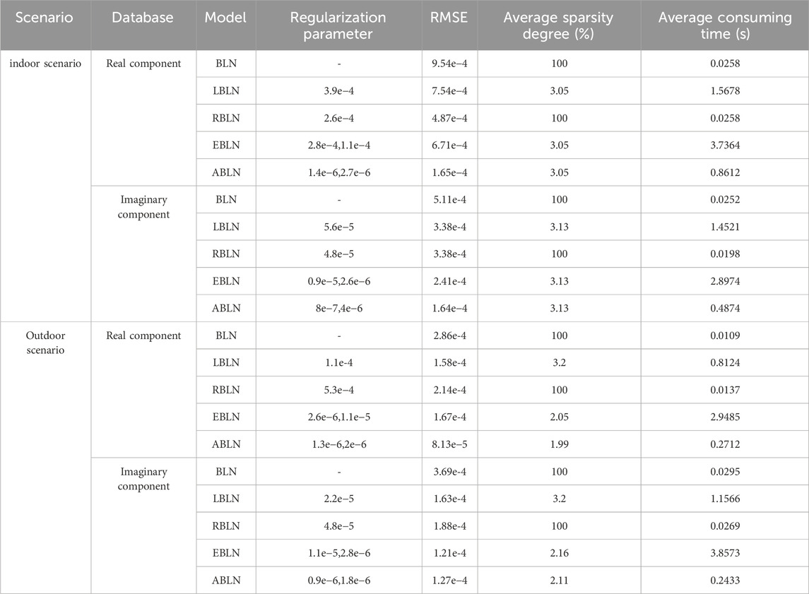
Table 2. One step prediction performance.

Table 3

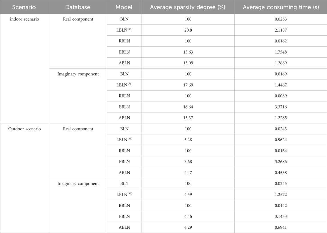
Table 3. Multistep prediction performance.

Figure 3

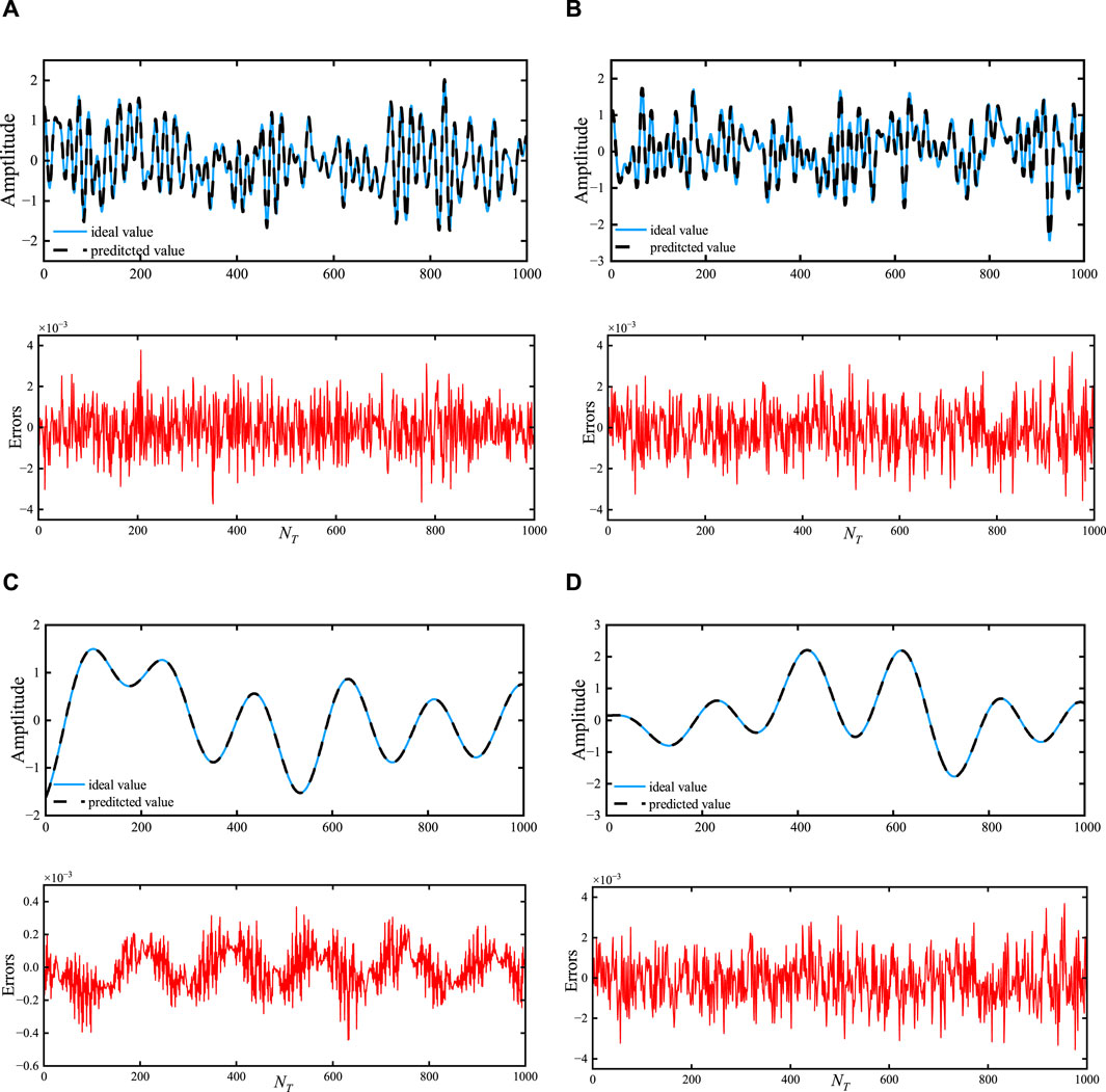
Figure 3. The predicted real and imaginary components of the inside scene are represented by the scenes (A,B), respectively, and the predicted real and imaginary elements of the outside scene by the scenes (C,D), respectively.

Figure 4

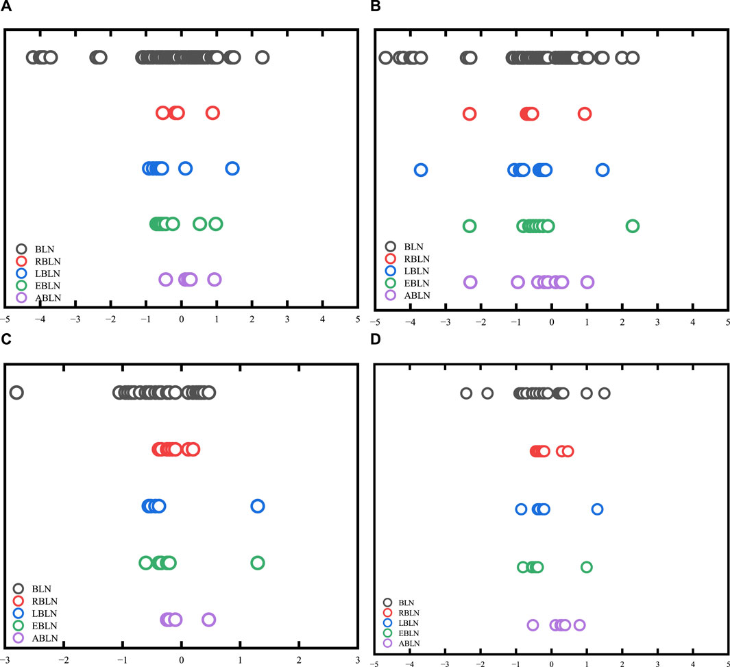
Figure 4. The estimated output weight matrix’s distribution range. in the indoor scene, (A,B) are the real and imaginary parts, respectively; (C,D) the real and imaginary parts in the outdoor scene.

The predicted CSI in ABLN, as illustrated in Figure 3A, closely resembles the ideal CSI with a maximum error of 2e-3, whereas Figure 3B shows a maximum error of 3e-3 for the imaginary component of the indoor scene. The correlation curves for the out-door scenario are displayed in Figures 3C, D. The predicted CSI curves, with a maximum error of 3e-4 in Figure 3C and 5e-3 for the imaginary component in Figure 3D, are observed to be satisfactorily accurate in matching the ideal curves. From Figure 3, it can be seen that ABLN has relatively small prediction errors in one step prediction of indoor scenes versus outdoor scenes compared to other models. Thus, for the CSI samples in the indoor scene and the outdoor scene, we can obtain excellent one step ABLN prediction performance. The one step prediction performance is shown in Table 2. Table 2 also includes the regularization parameters of the BLN-based models for the two scenarios. The assessed models’ average sparsity for the actual portion of the CSI samples in the in-door scenario is 3.05%, except for BLN and RBLN. But ABLN has the lowest RMSE (1.65e-4) compared to LESN (7.54e-4) and RESN (4.87e-3) and EESN (6.71e-4). It is calculated that, in terms of one step prediction performance, ABLN has a maximum improvement of about 96.49% with the other evaluated models. Furthermore, the amount of time needed to compute the output weight estimate matrix is also less in ABLN, with an average consumption time of about 0.8612 s, compared to 1.5678 s in LBLN and 3.7364 s in EBLN. Specifically, there is a considerable reduction in the computational time needed for the adaptive elasticity network in ABLN to estimate the input weight matrix. Although BLN and RBLN need less computing time (i.e., 0.0258), they do not yield a sparse output weight matrix. In the indoor situation, ABLN exhibits the best RMSE of 1.64e-4 and the same average sparsity of 3.13% for the imaginary part of the CSI samples. It also requires relatively little processing time, 0.4874 s. It is calculated that, in terms of the one step prediction performance, the maximum improvement of ABLN with respect to the other evaluated models is about 92.96%. ABLN requires smaller regularization parameters compared to other evaluation models. As a result, ABLN creates good sparse output weight matrices, has strong one step pre-diction performance, and uses less computing time to estimate the output weight matrices for CSI data in indoor environments. In the outdoor scenario, BLN exhibits the lowest performance for the genuine half of the CSI samples and requires a large amount of time to train the entire model; in contrast, ABLN requires very little computational time (0.2712 s) and has an ideal RMSE of 8.13e-5 and 1.99% mean sparsity. ABLN also has the same mean sparsity (e.g., 2.11%) for the imaginary component with an ideal RMSE (i.e., 1.27e-4), and a very short computation time (i.e., 0.2433 s). The highest improvement of the ABLN for the real and imaginary sections of these CSI samples compared to the other examined models in outdoor scenarios, is around 95.01% and 97.31% in terms of one step prediction performance. Therefore, ABLN can offer good one step prediction

Performance and shorter computing time for estimating the output weight matrices in two given communication scenarios for similar sparse output weight matrices.

Figure 4 displays the range of the estimated output weight matrix’s distribution in the BLN-based assessment model. The projected output weight matrix in BLN has a substantial size, as seen in Figure 4A, and it roughly ranges from −5 to 5. Thus indicating that the generalization ability of the input CSI samples is unsatisfactory. In addition, the output weight matrix of the BLN is not sparse. The output weight matrix of the RBLN is also not sparse, despite having an estimated output weight matrix with the smallest range of magnitude. Furthermore, even though the LBLN’s output weight matrix is sparse, its magnitude range exceeds the magnitude range of the RBLN. Com-pared with the output weight matrix of EBLN, the output weighting matrix typically approaches zero in ABLN. In terms of sparsity and magnitude range of the output weight matrix, ABLN has a clear advantage, which also indicates that ABLN has good generalization ability to the input CSI samples.

4.3 Multistep prediction

These parameters are the same as those in Table 3 for multi-step forecasts. Figure 5 displays the correlation curves for these assessed models’ 1-step to 15-step predictions for the two provided scenarios. Overall, the ABLN has the best multi-step prediction performance better compared to BLN, RBLN, LBLN and EBLN for the two given scenarios. In the indoor scenario, for the real and imaginary parts of the CSI samples, the improvement ratios of ABLN with the above evaluation models in the 15th step are about 80.14% and 82.03%, respectively, while in the outdoor scenario, these improvement ratios are about 90.87% and 97.42%, respectively. Moreover, ABLN has the best multi-step prediction performance for the BLN-based assessment model, particularly for the real portion of the CSI samples (Figures 5A, C). For the imaginary part of the two given scenes (as shown in Figures 5B, D), among the evaluation models, ABLN performs better in multi-step prediction. In the indoor scene, the 15th step prediction improvement rates of BLN-based ABLN compared to other evaluated models are approximately 35.28% and 28.94% for the real and imaginary parts of the CSI sample, respectively. Conversely, in the outdoor scene, these improvement rates are approximately 48.35% and 49.46%, respectively. Thus, as far as prediction performance is concerned, the ABLN has satisfactory multi-step performance for both real and imaginary parts in both given scenarios. The results for the evaluated models in terms of average sparsity and average time consumption are presented in Table 3. In this paragraph, the average sparsity and average consumption time are defined using the mean of predictions made across stages one through fifteen. In the indoor scenario, the output weight matrix in ABLN exhibits the optimal sparsity of 14.97% for the real part of the CSI samples, whereas the output weight matrices in BLN and BLN exhibit no sparsity. The BLN beats the other evaluation models, including the ABLN, in terms of the average time needed to estimate the output weight matrix. But as was already established, the BLN’s output weight matrix is not sparse. The conclusions are like those of the BLN. Then, the ABLN is also better in estimating the average time consumed for the output weight matrix compared to LBLN and EBLN. Therefore, the ABLN exhibits excellent multi-step prediction performance for the authentic portion of CSI data in the indoor scenario, considering both the average time required for calculating the output weight array and the sparsity of the estimated output weight matrix. The corresponding outcomes in the outdoor scenario are comparable to those obtained for the actual portion of CSI samples in the in-door scenario.

Figure 5

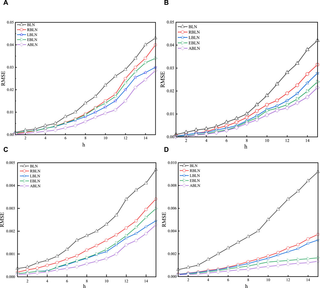
Figure 5. Multi-step prediction performance in indoor and outdoor scenarios: in the indoor scenario, (A,B) are real and imaginary parts, respectively; (C,D) real and imaginary parts in the outdoor scenario.

5 Conclusion

The channel prediction problem for distribution automation masters is the main topic of this study. Specifically, we propose in this study an ABLN for predicting the CSI of distribution automation master communications in OFDM systems. In this study, we simulate and analyze communication scenarios in both indoor and outdoor environments. The indoor scenario considers the Nakagami channel, while the outdoor scenario uses the Rayleigh channel. Moreover, in the simulation part, one step, multi-step and local predictability proofs for CSI samples are implemented. After the simulation, we draw several inferences. First, the CSI samples inferred by least squares (LS) in orthogonal frequency division multiplexing (OFDM) symbol subcarriers have significant local predictability, especially under the condition of finite maximum Doppler shift. In both cases, the local predictability of the best CSI samples exceeds 94.95%. Furthermore, in both cases, ABLN exhibits excellent one step and multistep prediction performance for both the real and imaginary parts of the CSI samples. In one step prediction, ABLN provides well one step prediction performance and shorter computation time to estimate the output weight matrix. In multistep prediction, ABLN provides satisfactory multistep performance in both real and imaginary parts of two given scenarios. It is characterised by sparse output weight matrices with small magnitude and less computational time required to estimate the output weight matrix, especially in one step prediction. The maximum improvement in the prediction performance of ABLN is calculated to be about 96.49% compared to other models. In addition, the regularization factor of ABLN is smaller than the regularization parameters of other evaluated models. Therefore, ABLN has advantages in channel prediction based on adaptive distribution automation master communication and can be used for future adaptive wireless communication in distribution automation master. The channel prediction method proposed in this paper can provide highly accurate channel prediction information, which provides a guarantee to reduce the impact of outdated channel state information on wireless communication systems such as distribution network automation master stations. The optimization and modification of the ABLN further to improve the prediction performances of the system model are the works in the future.

Data availability statement

The original contributions presented in the study are included in the article/Supplementary material, further inquiries can be directed to the corresponding author.

Author contributions

PL: Formal Analysis, Writing–original draft, Writing–review and editing. RZ: Investigation, Software, Writing–review and editing. HF: Data curation, Methodology, Writing–review and editing. HW: Resources, Validation, Visualization, Writing–review and editing. ZY: Data curation, Methodology, Supervision, Validation, Writing–review and editing.

Funding

The author(s) declare financial support was received for the research, authorship, and/or publication of this article. This research was funded by National Key Research and Development Program: Joint research and development and demonstration of collaborative energy management and operation optimization technology for “Belt and Road” National Urban Smart Energy Network (524608200157).

Conflict of interest

Authors PL, HF, and HW were employed by NARI Group Co., Ltd. Authors PL, HF, and HW were employed by NARI Technology Nanjing Control Systems Co., Ltd. Authors RZ and ZY were employed by Guangdong Power Grid Corporation.

Publisher’s note

All claims expressed in this article are solely those of the authors and do not necessarily represent those of their affiliated organizations, or those of the publisher, the editors and the reviewers. Any product that may be evaluated in this article, or claim that may be made by its manufacturer, is not guaranteed or endorsed by the publisher.

References

Bai, Q., Wang, J., Zhang, Y., and Song, J. (2019). Deep learning based channel estimation algorithm over time selective fading channels. IEEE T Cogn. Commun. 6, 125–134. doi:10.1109/TCCN.2019.2943455

CrossRef Full Text | Google Scholar

Chen, C. L. P., and Liu, Z. (2018). Broad learning system: an effective and efficient incremental learning system without the need for deep architecture. IEEE T Neur. Net. Lear. 29, 10–24. doi:10.1109/TNNLS.2017.2716952

PubMed Abstract | CrossRef Full Text | Google Scholar

Chen, C. L. P., Liu, Z., and Feng, S. (2019). Universal approximation capability of broad learning system and its structural variations. IEEE T Neur. Net. Lear. 30, 1191–1204. doi:10.1109/TNNLS.2018.2866622

PubMed Abstract | CrossRef Full Text | Google Scholar

Ding, H. F., Xie, Y. F., Xie, S. W., and Wang, J. (2023). A width learning system based on feature layer dense connectivity and attention mechanism and its application to zinc flotation process. Cont. Appli. 40, 111–120. doi:10.7641/CTA.2022.10753

CrossRef Full Text | Google Scholar

Ding, T., and Hirose, A. (2013). “Fading channel prediction based on complex-valued neural networks in frequency domain,” in IEEE International Symposium on Electromagnetic Theory, Hiroshima, Japan, May 2013, 640–643.

Google Scholar

Ding, T., and Hirose, A. (2014). Fading Channel prediction based on combination of complex-valued neural networks and chirp Z-transform. IEEE T Neur. Net. Lear. 25, 1686–1695. doi:10.1109/TNNLS.2014.2306420

CrossRef Full Text | Google Scholar

Duan, J. W., Xu, L. C., Quan, Y. J., Chen, L., and Chen, J. L. (2022). Bayesian width learning system based on graph regularization. J. Intelli. Sci. Tech. 4, 109–117. doi:10.11959/j.issn.2096–6652.202203

CrossRef Full Text | Google Scholar

Feng, S., and Chen, C. L. P. (2018). Fuzzy broad learning system: a novel neuro-fuzzy model for regression and classification. IEEE T Cy 99, 414–424. doi:10.1109/TCYB.2018.2857815

PubMed Abstract | CrossRef Full Text | Google Scholar

Gu, Y. (2017). Review of development status and trend of distribution automation in China. J. Electr. Engin 5, 270–277. doi:10.12677/jee.2017.54033

CrossRef Full Text | Google Scholar

Jiang, W., and Schotten, H. D. (2019). “Recurrent neural network-based frequency-domain Channel Prediction for wideband communications,” in IEEE Vehicular Technology Conference, Kuala Lumpur, Malaysia, April 2019, 1–9. doi:10.1109/VTCSpring.2019.8746352

CrossRef Full Text | Google Scholar

Jin, J. W., and Chen, C. L. P. (2018). Regularized robust Broad Learning System for uncertain data modeling. Neurocomputing 322, 58–69. doi:10.1016/j.neucom.2018.09.028

CrossRef Full Text | Google Scholar

Kapoor, D. S., and Kohli, A. K. (2018). Channel estimation and long-range prediction of fast fading channels for adaptive OFDM system. Int. J. Electron. Theor. Exp. 105, 1451–1466. doi:10.1080/00207217.2018.1460871

CrossRef Full Text | Google Scholar

Kurtz, R. B. S. A. (1987). Johan Håstad. Computational limitations of small-depth circuits. ACM doctoral dissertation awards. The MIT Press, Cambridge, Mass., and London, 1987, xiii + 84 pp. J. Symbolic Log. 53, 1259–1260. doi:10.2307/2274626

CrossRef Full Text | Google Scholar

Lee, J., Park, C., and Roh, H. (2021). “Revisiting bluetooth adaptive frequency hopping prediction with a ubertooth,” in international conference on information networking (ICOIN), Jeju Island, Korea (South), January 2021, 715–717. doi:10.1109/ICOIN50884.2021.9333996

CrossRef Full Text | Google Scholar

Liang, J. Y. (2023). Research on decentralized breadth learning system with high communication efficiency. Guilin Uni. Tech. doi:10.27050/d.cnki.gglgc.2023.001071

CrossRef Full Text | Google Scholar

Min, H., Shoubo, F., Philip, C. C. L., Meiling, X., and Tie, Q. (2018). Structured Manifold broad learning system: a Manifold perspective for large-scale chaotic time series analysis and prediction. IEEE T Knowl. Data En. 31, 1809–1821. doi:10.1109/TKDE.2018.2866149

CrossRef Full Text | Google Scholar

Muhammad, S. J. S., Huseyin, A. H., TurkmenHaji, M. F., and Arslan, H. (2021). Wireless communication, sensing, and REM: a security perspective. IEEE Open J. Commun. Soc. 2, 287–321. doi:10.1109/OJCOMS.2021.3054066

CrossRef Full Text | Google Scholar

Niu, G. Q., Yan, Y., Li, Y. C., Yao, X. J., Wang, C. M., and Gao, X. (2014). “Adaptive autoregressive prediction method for deep-space channel using kalman filter,” in 2014 IEEE International Conference on Instrumentation and Measurement, Computer, Communication and Control, Harbin, China, September 2014, 533–538.

CrossRef Full Text | Google Scholar

Pan, L., Han, Z., Shanshan, Z., and Feng, W. (2023). An optimal allocation method for power distribution network partitions based on improved spectral clustering algorithm. Int. J. Intelli. Real-Time Automation 123, 106497–106514. doi:10.1016/j.engappai.2023.106497

CrossRef Full Text | Google Scholar

Pao, Y. H., and Takefuji, Y. (2021). Functional-link net computing: theory, system architecture, and functionalities. Computer 25, 76–79. doi:10.1109/2.144401

CrossRef Full Text | Google Scholar

Pu, X., and Li, C. (2021). Online semi-supervised broad learning system for industrial fault diagnosis. IEEE T Ind. Inf. 17, 6644–6654. doi:10.1109/TII.2020.3048990

CrossRef Full Text | Google Scholar

Rodan, A., and Tino, P. (2012). Simple deterministically constructed cycle reservoirs with regular jumps. Neu. Compu. 24, 1822–1852. doi:10.1162/NECO_a_00297

PubMed Abstract | CrossRef Full Text | Google Scholar

Sarankumar, R., Poongodi, P., and Umamaheswari, G. (2016). Adaptive phase adjustment and Channel Prediction strategies (APA-CPS) in MIMO-OFDM based cognitive radios. Asian Journal of Information Technology 15 (11), 1816–1824.

Google Scholar

Schofield, D., Nagrani, A., Zisserman, A., Hayashi, M., Matsuzawa, T., Biro, D., et al. (2019). Chimpanzee face recognition from videos in the wild using deep learning. Sci. Adv. 5, eaaw0736–9. doi:10.1126/sciadv.aaw0736

PubMed Abstract | CrossRef Full Text | Google Scholar

Son, W. S., and Han, D. S. (2021). “Analysis on the Channel Prediction accuracy of deep learning-based approach,” in International Conference on Artificial Intelligence in Information and Communication (ICAIIC), Jeju Island, Korea, April 2021, 140–143. doi:10.1109/ICAIIC51459.2021.9415201

CrossRef Full Text | Google Scholar

Suganthan, P. N., and Katuwal, R. (2021). On the origins of randomization-based feedforward neural networks. Appl. Soft Com. 1, 107239–107245. doi:10.1016/j.asoc.2021.107239

CrossRef Full Text | Google Scholar

Tan, R. H., and Wang, J. (2023). Channel equalisation method for optical fibre communication networks based on deep learning networks. Laser J. 44, 157–161. doi:10.14016/j.cnki.jgzz.2023.10.157

CrossRef Full Text | Google Scholar

Trivedi, V. K., and Kumar, P. (2018). “BER performance of multi user scheduling for MIMO-OFDM and MIMO-SCFDMA broadcast network with imperfect CSI,” in National Conference on Communications, Hyderabad, India, February 2018, 1–6. doi:10.1109/NCC.2018.8599983

CrossRef Full Text | Google Scholar

Wang, G. (2022). A lightweight width learning system based on regularization and quantization techniques. China Uni. Min. Tech. doi:10.27623/d.cnki.gzkyu.2022.000296

CrossRef Full Text | Google Scholar

Wang, J., Ding, Y., Bian, S., Peng, Y., Liu, M., and Gui, G. (2019a). UL-CSI data driven deep learning for predicting DL-CSI in cellular FDD systems. IEEE Access 7, 96105–96112. doi:10.1109/ACCESS.2019.2929091

CrossRef Full Text | Google Scholar

Wang, T., Wen, C.-K., Jin, S., and Li, G. Y. (2019b). Deep learning-based CSI feedback approach for time-varying massive MIMO channels. IEEE Wirel. Commun. Lett. 8, 416–419. doi:10.1109/LWC.2018.2874264

CrossRef Full Text | Google Scholar

Xu, M., and Han, M. (2015). Adaptive elastic echo state network for multivariate time series prediction. IEEE T Cy 46, 2173–2183. doi:10.1109/TCYB.2015.2467167

PubMed Abstract | CrossRef Full Text | Google Scholar

Xue, C., Zhou, T., Zhang, H., Liu, L., and Tao, C. (2021). “Deep learning based Channel Prediction for massive MIMO systems in high-speed railway scenarios,” in 2021 IEEE 93rd Vehicular Technology Conference (VTC2021-Spring), Virtual Conference, April, 2021, 1–5. doi:10.1109/VTC2021-Spring51267.2021.9448982

CrossRef Full Text | Google Scholar

Yang, Y., Smith, D., Rajasegaran, J., and Seneviratne, S. (2020). Power control for body area networks: accurate Channel Prediction by lightweight deep learning. IEEE Internet Things 8, 3567–3575. doi:10.1109/JIOT.2020.3024820

CrossRef Full Text | Google Scholar

Zhang, T., Wang, X., Xu, X., and Chen, C. L. P. (2019). GCB-net: graph convolutional broad network and its application in emotion recognition. IEEE T Affect. Comput. 13, 379–388. doi:10.1109/TAFFC.2019.2937768

CrossRef Full Text | Google Scholar

Zhao, H., Zheng, J., Deng, W., and Song, Y. (2019). Semi-supervised broad learning system based on Manifold regularization and broad network. IEEE T Circuits-I 67, 983–994. doi:10.1109/TCSI.2019.2959886

CrossRef Full Text | Google Scholar

Zhao, H. Q., and Lu, X. (2023). Width learning system based on generalised maximum correlation entropy criterion. Signal Process., 1–7. doi:10.16798/j.issn.1003-0530.2023.11.005

CrossRef Full Text | Google Scholar

Zhou, D. X. (2013). On grouping effect of elastic net. Sta. Proba. Lett. 83, 2108–2112. doi:10.1016/j.spl.2013.05.014

CrossRef Full Text | Google Scholar