Numerical modeling of mixed convective nanofluid flow with fractal stochastic heat and mass transfer using finite differences

This study presents the first comprehensive numerical simulation of heat and mass transfer in fractal-like mixed convective nanofluid flows. The flow of non-Newtonian nanofluids over flat and oscillating sheets is modelled mathematically, and a finite difference scheme is used to solve this model. The two-stage scheme can tackle fractal and fractal stochastic mathematical models of partial differential equations. The consistency in the mean square is proved, and Fourier series stability analysis is adopted to find stability conditions for fractal stochastic partial differential equation. The scheme is applied to solve the unsteady Casson nanofluid flow over the flat and oscillatory sheet, which affects thermal radiation, heat source, and chemical reaction. The existence of the solution is also provided for the Navier-Stokes equation of the considered flow model using fractal time derivative. The graph illustrates that the proposed fractal technique achieves faster convergence than the Crank-Nicolson approach. Applications in energy systems, materials science, and environmental engineering are just a few of the domains that could benefit from a better understanding of mixed convective nanofluid flows with fractal features, and that is what this research study hopes to accomplish. Scientists and engineers may better develop efficient and environmentally friendly systems by simulating and analyzing these complicated processes with the suggested finite difference technique.

1 Introduction

Fluid dynamics have always been one of the most fascinating topics in the field of science. This area mainly studies different types of liquids or gases and their flowing condition in further investigations. There are three subparts to fluid dynamics: fractals, stochastic, and non-Newtonian flow. These subdivisions are now inspiring new research areas with the potential to have a range of practical and engineering uses.

Fractal fluid flow can be explained as a fluid system’s self-similar fragmented patterns and structures. Many natural and artificial systems showed fractals, including weather, stream, internet connectivity, and blood vessel networks in biological systems. It does not matter what magnification or loss of detail you choose; they will let you find the exact shape several times. Using the rule for limited design, impracticable shapes can be constructed from the principles of fractal fluid flow.

Fractals have an enormous role to play in fluid mechanics. A study that identifies the number of fractals almost widely known by the public proves an essential part of fluid flows, such as combustion (Sreenivasan, 1991), irregular flow (Sreenivasan and Meneveau, 1986; Gouldin, 1987; Ueki et al., 1999; Mazzi and Vassilicos, 2004; Cintosum et al., 2007), and fluid mechanics in general (Anwar, 2019; Anwar, 2020; Ahmad Sheikh et al., 2021; Anwar et al., 2024).

Various exciting properties of fractals have been found relative to fluid dynamics in recent years. A numerical study of the Navier-Stokes equations resulted in a few researchers (Lanotte et al., 2015) investigating the intermittency’s origin in an incompressible, homogeneous, and isotropic turbulent flow. Another had also been carried out (Lanotte et al., 2016) for incompressible, homogeneous, and isotropic turbulent flow. This is achieved by solving the Navier-Stokes equations using a restricted set of Fourier modes, which are part of a fractal set characterized by dimension $D$. The term “incompressible” refers to a substance or material exhibiting negligible change. The Navier-Stokes equations represent an incompressible fluid’s dynamic motion or flow. These equations express the unknowns of velocity and pressure as functions of both spatial and temporal variables. As mentioned earlier, the solution to the equations enables predicting the fluid’s behaviour, contingent upon understanding its initial and boundary conditions. The above equations are important as fundamental models within mathematical physics (Łukaszewicz et al., 2016). Although numerous research investigations have yielded critical preliminary stages and approaches, their answers remain one of applied mathematics’s most fundamental and challenging problems. Among these methods are fractal geometry and fractional calculus. Most of the solutions of the resulting fractional equations of motion are not trivial, even though the fractional nonlocal approach is very inspiring and has many exciting features, especially in continuum mechanics (Rasheed and Anwar, 2018; Hussain et al., 2021), hydrodynamics (Ali et al., 2021a; Ali et al., 2021b), and magnetohydrodynamics (Song and Em Karniadakis, 2019), etc. Therefore, it is necessary to make solution estimations using numbers.

The study’s objective (Kumar et al., 2014) is to present a novel analytical and approximation method for solving the time-fractional Navier-Stokes equation (NSE) within a cylindrical conduit. The suggested methodology integrates the Adomian decomposition (ADM) and the Laplace transform (LTM). Analytical solutions to the time-fractional Navier-Stokes equations are established by modifying the reduced differential transform method and developing a new iterative Elzaki transform method, both of which are shown in (Wang and Liu, 2016). In reference (Khan et al., 2009), the use of the Caputo fractional derivative is employed to investigate the Navier-Stokes equation with fractional orders using He’s homotopy perturbation technique (HPM) and variational iteration method (VIM). These approaches provide novel avenues for addressing NSE, although they are limited in several technical respects.

Fractal calculus, first introduced in (Parvate and Gangal, 2009; Gangal et al., 2011; Parvate and Gangal, 2011), provided more possibilities and feasible solutions to NSE in (Pishkoo and Darus, 2021). Since the Hausdorff fractal dimension has been shown to have a significant role in the NSE-governed flow of viscous incompressible fluids (Scheffer, 1978; Babin and Vishik, 1985; Shah and Abdeljawad, 2024), this makes intuitive sense. In (Kukavica, 2009), weak solutions of the NSE in a space-time fractal domain with finite dimensions were investigated. Using stochastic differential equations driven by Levy processes, the authors of (Zhang, 2012) explain a stochastic Lagrangian particle route method to NSE in detail. In (Constantin et al., 1985), approximate solutions of NSE in terms of time are provided for fractal dimensions, while in (Hinz and Teplyaev, 2015), NSE on one-dimensional topological fractals is studied using Hodge theory. In (Yang et al., 2020), the pullback attractors for 2D non-autonomous incompressible NSE with constant delay terms were investigated, and their limited fractal and Hausdorff dimensions were determined. The NSE was also investigated in fractal dimensions of invariant sets (Chepyzhov and Llyin, 2014). In (Mahalov et al., 1990), we derive estimates for the Hausdorff and fractal dimensions of the NSE global attractors based on the spiral and regulating physical parameters. Fractals and fractal dimensions are significant to these and other studies in fluid mechanics.

On the other side, stochastic fluid flow explores the world of chance and uncertainty in fluid systems. Fluid behaviour under varying forces or situations can be analyzed and predicted using probabilistic and statistical ideas. Stochastic modelling has proven beneficial in the face of difficulties in predicting weather and analyzing the behaviour of fluid particles in turbulence. Improvements in forecasting, risk assessment, and policymaking in domains as disparate as climate science and the stock market can be traced back to the lessons learned from research into stochastic fluid flow.

Of all the deterministic equations in physics that hide unpredictability, the most famous one is the Schrödinger equation. No mathematical probability theory can account for the inherent randomness in a quantum physics lab. Regardless of this seeming contradiction, Quantum Theory has produced a robust set of tools for controlling specific types of randomness, namely the departure from classical motion equation solutions. Does this classical/quantum link affect the Navier-Stokes and Euler equations? The two hydrodynamic equations differ significantly from the ones mentioned earlier. Euler Equation, even though representing “dry water” (Von Neumann) is already very complicated. At this moment, there seems to be no proof that it refrains from producing singularities. The comparison, as mentioned above, however, has the potential to provide some intriguing details regarding the turbulence development process.

There are several entry points for uncertainty, including faulty initial conditions. Here, statistical methods are considered: one looks at the development of a probability measure over time-based on the pertinent physical beginning facts and initiated in the 19th century (see, among many others, (Vishik et al., 1979; Marchioro and Pulvirenti, 1984). Stochastic diffusion processes have been devised for several kinds of Langevin dynamics, including equilibrium and non-equilibrium dynamics, including Kraichnan’s model in turbulent advection (for instance, see (Gawedzki et al., 2008)). To learn more about how numerical models could contribute to uncertainty, check out (Palmer and Williams, 2008; Crisan et al., 2019) about climate modelling.

Stochastic partial differential equations (SPDEs) are another well-known way to include stochasticity into the Navier-Stokes equation by including random forces. There is a mountain of material on the subject since the first seminal mathematical work on it (Bensoussan and Teman, 1973). Turbulence has been used to study stochastic Lagrangian models of the Langevin type, which incorporate smooth Lagrangian trajectories and random velocities. However, it is essential to note that such models are not commonly employed in this field (Pope, 1994).

Recently, D. D. Holm developed stochastic advection through Lie transfer (Holm, 2015). Since this is an Eulerian method, the resulting equations of motion are SPDEs.

It would be impossible to provide a comprehensive list of all the stochastic approaches that may be used to analyze fluid dynamics. Only a small subset of topics and supporting references have been selected. It is worthwhile to highlight a few interesting probabilistic representation equations. Solutions to partial differential equations are typically represented in stochastic analysis as the expected values of functionals of stochastic processes. This method has been used for a long time and is also investigated for fluid dynamics. In (Busnello, 1999), for example, a probabilistic description of the vorticity field is presented; in (le Jan and Sznitman, 1997), branching processes and the Fourier transform are used for analysis; and in (Constantin and Iyer, 2008), Lagrangian diffusion processes are employed.

Non-Newtonian fluids, particularly those with yield stress, can describe their behaviour using the Casson fluid flow mathematical model. The rheological properties of such fluids can be described by the Casson equation, which British rheologist Sydney Goldstein Casson developed. Non-Newtonian fluids, such as Casson fluids, have more complicated flow properties than Newtonian fluids, which show a linear relationship between shear stress and shear rate. Casson fluids are distinguished by their dual nature as an elastic solid and a viscous liquid.

Food processing, medicines, paints, and drilling fluids are just a few industries that can benefit from Casson fluid flow. It is essential to optimize production processes and create effective transportation networks by having a firm grasp on the flow behaviour of Casson fluids.

The flow of Casson fluids in various geometries and under various situations is studied by researchers and engineers using numerical simulations and experimental methods. Predicting flow behaviour, calculating pressure drops, and building suitable apparatus for handling Casson fluids all benefit from these findings.

Coating applications benefit significantly from Casson multiphase suspensions due to the many engineering uses for thick multiphase flows, such as in the chemical and textile industries (Batra and Jena, 1991). In addition, the worst-case scenario of magnetized multiphase flows is used to validate the prior work. The circulation of blood via the body’s arteries is a well-known example of the Casson fluid flow model (Srivastava and Saxena, 1994), among other cutting-edge applications of this model (Das and Batra, 1993). Several newly developed and repurposed delivery systems use this technique, one of which is conveying cells to the brain. Non-Newtonian fluids are seeing increased use in engineering and production. Biomechanics and polymer processing heavily use the Casson fluid model (Dash et al., 1996) to depict non-Newtonian fluid dynamics (Eldabe et al., 2001).

One category of non-Newtonian fluids whose features include yield stress is the Casson fluid model. Jelly, honey, sauce, concentrated fruit liquids, soup, etc., all feature Casson fluid as an ingredient. In addition, it has many other expanding uses in various industries. The non-Newtonian fluid’s dynamic and complicated character and interactions make its study more challenging. The zero shear stress at infinite viscosity of Casson fluid classifies it as a dilatant fluid. If the yield stress exceeds the applied stress, the fluid exhibits solid-like behaviour; conversely, if the yield stress is lower, the fluid demonstrates liquid-like characteristics. The Casson fluid model equation was initially introduced by Casson in his work (Casson, 1959). This model’s creation drew the attention of numerous scientists intent on finding a solution to the issue. The movement of Casson nanofluid along the stretching sheet was analyzed by Abbas and Shatanawi (Abbas and Shatanawi, 2022). In their study of Casson nanofluids with convective boundary conditions, Nadeem et al. (Nadeem et al., 2013) emphasized the role played by magnetic hydrodynamics. Brownian motion and thermophoresis were also brought up for discussion. At a stretching sheet, Oyelakin et al. (Oyelakin et al., 2016) investigated the time-dependent flow of Casson fluid. Thermal radiation, slip, and convective boundary conditions were investigated. Brownian motion and thermophoresis were also shown to have an impact. By considering chemical reactions and buoyancy effects across the wedge, this study aims to analyze the flow properties of a Casson liquid in a two-dimensional (2D) laminar continuous flow via a stretched porous wedge (Hussain et al., 2023). Casson micropolar fluid flow at a curved surface was considered by Amjad et al. (Amjad et al., 2020). They talked about Brownian and thermophoresis motion in induced magnetic hydrodynamics. Triple solutions of Casson nanofluid were examined by Lanjwani et al. (Lanjwani et al., 2021) at the vertical nonlinear stretching sheet. Several researchers have investigated how different physical characteristics change when the flow assumption is made with artificial neural networks (for example, see Refs. (Shafiq et al., 2022; Çolak et al., 2022; Shafiq et al., 2023)).

We began an exciting adventure into complexity, uncertainty, and fluid flow interactions as we investigated fractal, stochastic, and Casson fluid flow. Scientists and engineers are deciphering the complexities of fluid dynamics through cross-disciplinary study and novel applications, thereby expanding the boundaries of human understanding and propelling progress that could change many other fields. We explore these fascinating areas further to learn more about them and use their enormous potential for the greater good of humanity. This study hints at a complex and niche area of computational fluid dynamics and heat transfer, particularly relating to nanofluids and fractal stochastic processes. Some real-world uses and ramifications of this study are as follows:

1. This study can potentially improve the design of heat shields, thermal protection systems, and cutting-edge cooling methods for spacecraft and aeroplanes used in the aerospace industry, where extreme temperatures are often experienced.

2. The fractal stochastic component of this study has potential use in weather prediction and climate simulation. Accurate and precise climate models and weather forecasts can be provided by comprehensively understanding heat and mass transfer in the intricate turbulent context.

3. Nanofluids are specific colloid suspensions with the particles (in nanoparticle form) carefully spread uniformly in the base fluid. The study presented here can provide detailed information about the process. It can, therefore, be helpful in the field of nanofluid technology for a significant understanding of heat and mass transport.

This study can be beneficially employed across various industrial fields and applications. For instance, in technological, engineering, medical, and environmental science, this study can be implemented to advance the efficiency and performance of various systems and devices in the field of cooling systems. Moreover, this needs to be considered for elaborative analysis in spacecraft, industry, electronics, etc.

In literature, much work exists on solving the flow problems over some surfaces. However, this work considers a stochastic model using the fractal time derivative. The model has been solved by the finite difference scheme that solves the given Equation in two stages. The solution is found first on arbitrary time and then on the next time level. For this work, the iterative method solves those difference equations obtained by applying the proposed fractal scheme to the considered flow model. The iterative technique employs a single initial approximation and determines the answer of the subsequent iteration by considering the solution computed during the previous iteration.

To conclude, in our paper, we have to introduce fractal characteristics with numerical simulation for the first time in the study of the mixed convective nanofluid flow. We are unaware of any other research incorporating fractal and fractal stochastic mathematical models in examining non-Newtonian nanofluid’s heat and mass flow on a flat surface and an oscillating sheet. Our fractal approach projects evidence of faster convergence compared to the traditional Crank-Nicolson solution technique. Our two-stage finite difference scheme can also use the fractal framework for the standard linear equation problem. We are also studying the unsteady Casson nanofluid flow in the presence of thermal radiation, an extensive heat source, and a reacting, homogeneous and endothermic chemical reaction. Our findings are not limited to heat and mass transference in nanofluid, as we believe it would benefit various energy systems, materials, and the environment.

2 Proposed computational scheme

A numerical scheme will be proposed to solve fractal SPDEs. The scheme will be a predictor-corrector type scheme, with the first stage as the predictor and explicit scheme. The scheme is the explicit-implicit scheme. For proposing a scheme for partial differential equations (PDEs), consider the FPDEs as follows:

$\frac{\partial v}{\partial t^{\alpha }}=F\left(v,\frac{{\partial }^{2}v}{\partial y^2}\right)(1)$

where $0<\alpha <1$.

Let the first stage of the scheme be expressed as:

${\overline{v}}_i^{n+1}=v_i^n+\Delta t\frac{\alpha }{t_n^{1-\alpha }}{\left(\frac{\partial v}{\partial t^{\alpha }}\right)}_i^n(2)$

Where $\Delta t$ is the temporal step size.

The second stage for discretizing the time variable of Eq. 1 can be expressed as:

$v_i^{n+1}=\frac{1}{10}\left(v_i^n+9{\overline{v}}_i^{n+1}\right)+\Delta t\frac{\alpha }{t_n^{1-\alpha }}\left[a{\left(\frac{\partial v}{\partial t^{\alpha }}\right)}_i^{n+1}+b{\left(\frac{\partial v}{\partial t^{\alpha }}\right)}_i^n+c{\left(\frac{\partial \overline{v}}{\partial t^{\alpha }}\right)}_i^{n+1}\right](3)$

Where $a,b$ and $c$ are unknown parameters. For finding $a,b$ and $c,$ re-write Eq. 3 as:

$v_i^{n+1}=\frac{1}{10}\left(v_i^n+9{\overline{v}}_i^{n+1}\right)+\Delta t\frac{\alpha }{t_n^{1-\alpha }}\left[a\frac{t_{n+1}^{1-\alpha }}{\alpha }{\left(\frac{\partial v}{\partial t}\right)}_i^{n+1}+b{\frac{t_n^{1-\alpha }}{\alpha }\left(\frac{\partial v}{\partial t}\right)}_i^n+c\frac{{\overline{t}}^{1-\alpha }}{\alpha }{\left(\frac{\partial \overline{v}}{\partial t}\right)}_i^{n+1}\right](4)$

where ${\overline{t}}^{1-\alpha }=\frac{t_n^{1-\alpha }+t_{n+1}^{1-\alpha }}{2}$.

Consider the Taylor series expansion for $v_i^{n+1}$ and ${\left(\frac{\partial v}{\partial t}\right)}_i^{n+1}$

$v_i^{n+1}=v_i^n+\Delta \mathrm{t}{\left(\frac{\partial v}{\partial t}\right)}_i^n+\frac{{\left(\Delta t\right)}^2}{2}{\left(\frac{{\partial }^{2}v}{\partial t^2}\right)}_i^n+\frac{{\left(\Delta t\right)}^3}{6}{\left(\frac{{\partial }^{3}v}{\partial t^3}\right)}_i^n+o\left({\left(\Delta t\right)}^4\right)(5)$

${\left(\frac{\partial v}{\partial t}\right)}_i^{n+1}={\left(\frac{\partial v}{\partial t}\right)}_i^n+\Delta t{\left(\frac{{\partial }^{2}v}{\partial t^2}\right)}_i^n+\frac{{\left(\Delta t\right)}^2}{2}{\left(\frac{{\partial }^{3}v}{\partial t^3}\right)}_i^n+o\left({\left(\Delta t\right)}^3\right)(6)$

Substituting expression for $v_i^{n+1}$ and ${\left(\frac{\partial v}{\partial t}\right)}_i^{n+1}$ into Eq. 4, it is obtained

$\begin{array}{l}{v}_i^n+\Delta \mathrm{t}{\left(\frac{\partial v}{\partial t}\right)}_i^n+\frac{{\left(\Delta t\right)}^2}{2}{\left(\frac{{\partial }^{2}v}{\partial t^2}\right)}_i^n+\frac{{\left(\Delta t\right)}^3}{6}{\left(\frac{{\partial }^{3}v}{\partial t^3}\right)}_i^n=\frac{1}{10}\left(v_i^n+9{\left(\frac{\partial v}{\partial t}\right)}_i^n\right)\\ +\Delta t\frac{\alpha }{t_n^{1-\alpha }}\left[a\frac{t_{n+1}^{1-\alpha }}{\alpha }{\left(\frac{\partial v}{\partial t}\right)}_i^n+a\Delta t\frac{t_{n+1}^{1-\alpha }}{\alpha }{\left(\frac{{\partial }^{2}v}{\partial t^2}\right)}_i^n+\frac{{\left(\Delta t\right)}^2}{2}a\frac{t_{n+1}^{1-\alpha }}{\alpha }{\left(\frac{{\partial }^{3}v}{\partial t^3}\right)}_i^n+b{\frac{t_n^{1-\alpha }}{\alpha }\left(\frac{\partial v}{\partial t}\right)}_i^n+c\frac{{\overline{t}}^{1-\alpha }}{\alpha }{\left(\frac{\partial v}{\partial t}\right)}_i^n+c\Delta t\frac{{\overline{t}}^{1-\alpha }}{\alpha }{\left(\frac{{\partial }^{2}v}{\partial t^2}\right)}_i^n\right]\end{array}(7)$

When comparing the coefficients of $\Delta t{\left(\frac{\partial v}{\partial t}\right)}_i^n,{\left(\Delta t\right)}^2{\left(\frac{{\partial }^{2}v}{\partial t^2}\right)}_i^n$ and ${\left(\Delta t\right)}^3{\left(\frac{{\partial }^{3}v}{\partial t^3}\right)}_i^n$ on both sides of Eq. 7 gives

$a=\frac{1}{3}\frac{t_n^{1-\alpha }}{t_{n+1}^{1-\alpha }}(8)$

$b=-\frac{2}{5}(9)$

$c=\frac{1}{6}\frac{t_n^{1-\alpha }}{{\overline{t}}^{1-\alpha }}.(10)$

Therefore, Eq. 2 and (3) using (8), (9) and (10) gives the numerical scheme that discretizes the fractal time variable of Eq. 1.

The scheme given in (2) and 3 can be extended from fractal PDE (1) to fractal stochastic PDE.

$dv=G\left(v,{\partial }_{xx}v\right)d{t}^{\alpha }+\sigma dW(11)$

is

${\overline{v}}_i^{n+1}=v_i^n+\Delta tG\left(v_i^n,{\partial }_{xx}{v}_i^n\right)(12)$

$v_i^{n+1}=\frac{1}{10}\left(v_i^n+9{\overline{v}}_i^{n+1}\right)+\Delta t\frac{\alpha }{t_n^{1-\alpha }}\left[aG\left(v_i^{n+1},{\partial }_{xx}{v}_i^{n+1}\right)\frac{t_{n+1}^{1-\alpha }}{\alpha }+bG\left(v_i^n,{\partial }_{xx}{v}_i^n\right)\frac{t_n^{1-\alpha }}{\alpha }+cG\left({\overline{v}}_i^{n+1},{\partial }_{xx}{\overline{v}}_i^{n+1}\right)\frac{{\overline{t}}^{1-\alpha }}{\alpha }\right]+\sigma \left(W^{n+1}-W^n\right)(13)$

For $G={\partial }_{xx}v$ scheme (12) and (13) is given as:

${\overline{v}}_i^{n+1}=v_i^n+\Delta t\left(\frac{v_{i+1}^n-2v_i^n+v_{i-1}^n}{{\left(\Delta x\right)}^2}\right)(14)$

$v_i^{n+1}=\frac{1}{10}\left(v_i^n+9{\overline{v}}_i^{n+1}\right)+\Delta t\frac{\alpha }{t_n^{1-\alpha }}\left[a\frac{t_{n+1}^{1-\alpha }}{\alpha }\left(\frac{v_{i+1}^{n+1}-2v_i^{n+1}+v_{i-1}^{n+1}}{{\left(\Delta x\right)}^2}\right)+b\frac{t_n^{1-\alpha }}{\alpha }\left(\frac{v_{i+1}^n-2v_i^n+v_{i-1}^n}{{\left(\Delta x\right)}^2}\right)+c\frac{{\overline{t}}^{1-\alpha }}{\alpha }\left(\frac{{\overline{v}}_{i+1}^{n+1}-2{\overline{v}}_i^{n+1}+{\overline{v}}_{i-1}^{n+1}}{{\left(\Delta x\right)}^2}\right)\right]+\sigma \Delta W(15)$

where $\Delta W\sim N\left(0,\sqrt{\Delta t}\right)$.

Eqs. 14 and (15) give the time and space discretization of fractal stochastic Eq. 11 where $G={\partial }_{xx}v$. To find the consistency and stability of fractal stochastic Equation, consider the following Equation:

$dv=d_1{\partial }_{xx}vd{t}^{\alpha }+\sigma vdW(16)$

The time and space discretization of Eq. 16 using the proposed scheme is given as:

${\overline{v}}_i^{n+1}=v_i^n+\Delta t\left[d_1\left(\frac{v_{i+1}^n-2v_i^n+v_{i-1}^n}{{\left(\Delta x\right)}^2}\right)\right](17)$

and

$v_i^{n+1}=\frac{1}{10}\left(v_i^n+9{\overline{v}}_i^{n+1}\right)+\Delta t\frac{\alpha }{t_n^{1-\alpha }}\left[a\frac{t_{n+1}^{1-\alpha }}{\alpha }{d}_1\left(\frac{v_{i+1}^{n+1}-2v_i^{n+1}+v_{i-1}^{n+1}}{{\left(\Delta x\right)}^2}\right)+b\frac{t_n^{1-\alpha }}{\alpha }{d}_1\left(\frac{v_{i+1}^n-2v_i^n+v_{i-1}^n}{{\left(\Delta x\right)}^2}\right)+c\frac{{\overline{t}}^{1-\alpha }}{\alpha }{d}_1\left(\frac{{\overline{v}}_{i+1}^{n+1}-2{\overline{v}}_i^{n+1}+{\overline{v}}_{i-1}^{n+1}}{{\left(\Delta x\right)}^2}\right)\right]+\sigma v_i^n\Delta W(18)$

Theorem 1. The numerical scheme given in (17) and 18 is consistent in the mean square sense.

Proof: Let $P$ be a smooth function, then

$L{\left(P\right)}_i^n=P\left(\left(n+1\right)\Delta t,i\Delta x\right)-P\left(n\Delta t,i\Delta x\right)-{\int }_{n\Delta t}^{\left(n+1\right)\Delta t}{P}_{xx}\left(s,i\Delta x\right)ds-\sigma {\int }_{n\Delta t}^{\left(n+1\right)\Delta t}P\left(s,i\Delta x)dW(s\right)(19)$

$\begin{array}{l}L{\left(P\right)}_i^n=P\left(\left(n+1\right)\Delta t,i\Delta x\right)-P\left(\mathrm{n}\Delta t,i\Delta x\right)-\frac{\Delta t}{{\left(\Delta x\right)}^2}\\ \frac{\alpha }{t_n^{1-\alpha }}\left[a\frac{t_{n+1}^{1-\alpha }}{\alpha }{d}_1\left(P\left(\left(n+1\right)\Delta t,\left(i+1\right)\Delta x\right)-2P\left(\left(n+1\right)\Delta t,i\Delta x\right)+P\left(\left(n+1\right)\Delta t,\left(i-1\right)\Delta x\right)\right)\right]\\ +\left(b+\frac{9}{10}\right)\frac{t_n^{1-\alpha }}{\alpha }{d}_1\left(P\left(n\Delta t,\left(i+1\right)\Delta x\right)-2P\left(n\Delta t,i\Delta x\right)+P\left(n\Delta t,\left(i-1\right)\Delta x\right)\right)\\ \left.+c\frac{{\overline{t}}^{1-\alpha }}{\alpha }\left(\overline{P}\left(\left(n+1\right)\Delta t,\left(i+1\right)\Delta x\right)-2\overline{P}\left(\left(n+1\right)\Delta t,i\Delta x\right)+\overline{P}\left(\left(n+1\right)\Delta t,\left(i-1\right)\Delta x\right)\right)\right]\\ -\sigma P\left(s,i\Delta x\right)\left(W\left(\left(n+1\right)\Delta t\right)-W\left(n\Delta t\right)\right)\end{array}(20)$

where $\overline{P}\left(\left(n+1\right)\Delta t,i\Delta x\right)=P\left(\mathrm{n}\Delta t,i\Delta x\right)+\frac{\Delta t}{{\left(\Delta x\right)}^2}{d}_1\left(P\left(n\Delta t,\left(i+1\right)\Delta x\right)-2P\left(n\Delta t,i\Delta x\right)+P\left(n\Delta t,\left(i-1\right)\Delta x\right)\right)$

$\begin{array}{l}E{\left|L{\left(P\right)}_i^n-L_i^{n}P\right|}^2=E|-d_1{\int }_{n\Delta t}^{\left(n+1\right)\Delta t}{P}_{xx}\left(s,i\Delta x\right)ds-\sigma {\int }_{n\Delta t}^{\left(n+1\right)\Delta t}P\left(s,i\Delta x\right)dW\left(s\right)\\ +\frac{\Delta t}{{\left(\Delta x\right)}^2}\frac{\alpha }{t_n^{1-\alpha }}[a\frac{t_{n+1}^{1-\alpha }}{\alpha }{d}_1\left(P\left(\left(n+1\right)\Delta t,\left(i+1\right)\Delta x\right)-2P\left(\left(n+1\right)\Delta t,i\Delta x\right)+P\left(\left(n+1\right)\Delta t,\left(i-1\right)\Delta x\right)\right)\\ +\left(b+\frac{9}{10}\right)\frac{t_n^{1-\alpha }}{\alpha }{d}_1\left(P\left(n\Delta t,\left(i+1\right)\Delta x\right)-2P\left(n\Delta t,i\Delta x\right)+P\left(n\Delta t,\left(i-1\right)\Delta x\right)\right)\\ +c\frac{{\overline{t}}^{1-\alpha }}{\alpha }\left(\overline{P}\left(\left(n+1\right)\Delta t,\left(i+1\right)\Delta x\right)-2\overline{P}\left(\left(n+1\right)\Delta t,i\Delta x\right)+\overline{P}\left(\left(n+1\right)\Delta t,\left(i-1\right)\Delta x\right)\right)]+\sigma P\left(s,i\Delta x\right)\left(W\left(\left(n+1\right)\Delta t\right)-W\left(n\Delta t\right)\right){|}^2\end{array}(21)$

Eq. 21 can be expressed as:

$\begin{array}{l}E{\left|L{\left(P\right)}_i^n-L_i^{n}P\right|}^2\le 2d_1^{2}E\left|\right[{\int }_{n\Delta t}^{\left(n+1\right)\Delta t}{P}_{xx}\left(s,i\Delta x\right)ds-\frac{\Delta t}{{\left(\Delta x\right)}^2}\frac{\alpha }{t_n^{1-\alpha }}\\ \left\{a||\frac{t_{n+1}^{1-\alpha }}{\alpha }|\left(P\left(\left(n+1\right)\Delta t,\left(i+1\right)\Delta x\right)-2P\left(\left(n+1\right)\Delta t,i\Delta x\right)+P\left(\left(n+1\right)\Delta t,\left(i-1\right)\Delta x\right)\right)\right.\\ +\left(b+\frac{9}{10}\right)\frac{t_n^{1-\alpha }}{\alpha }\left(P\left(n\Delta t,\left(i+1\right)\Delta x\right)-2P\left(n\Delta t,i\Delta x\right)+P\left(n\Delta t,\left(i-1\right)\Delta x\right)\right)\\ \left.+|c||\frac{{\overline{t}}^{1-\alpha }}{\alpha }|\left(\overline{P}\left(\left(n+1\right)\Delta t,\left(i+1\right)\Delta x\right)-2\overline{P}\left(\left(n+1\right)\Delta t,i\Delta x\right)+\overline{P}\left(\left(n+1\right)\Delta t,\left(i-1\right)\Delta x\right)\right)\right\}]{|}^2\\ +2{\sigma }^{2}E{\left|{\displaystyle \underset{n\Delta t}{\overset{\left(n+1\right)\Delta t}{\int }}}\left[P\left(s,i\Delta x\right)-P\left(s,i\Delta x\left)\right]dWs\right)\right.\right|}^2\end{array}(22)$

Using the inequality

$E{\left|{\int }_{t_{\circ }}^{t}g\left(s,k\right)dW\left(s\right)\right|}^{2n}\le {\left(t-t_{\circ }\right)}^{n-1}{\left\{n\left(2n-1\right)\right\}}^n{\int }_{t_{\circ }}^{t}E\left\{{\left|f\left(s,k\right)\right|}^{2n}\right\}ds(23)$

Inequality (22) can be written as

$\begin{array}{l}E{\left|L{\left(P\right)}_i^n-L_i^{n}P\right|}^2\le 2d_1^{2}E\left|\right[{\int }_{n\Delta t}^{\left(n+1\right)\Delta t}{P}_{xx}\left(s,i\Delta x\right)ds-\frac{\Delta t}{{\left(\Delta x\right)}^2}\frac{\alpha }{t_n^{1-\alpha }}\left\{a\frac{t_{n+1}^{1-\alpha }}{\alpha }\left(P\left(\left(n+1\right)\Delta t,\left(i+1\right)\Delta x\right)-2P\left(\left(n+1\right)\Delta t,i\Delta x\right)+P\left(\left(n+1\right)\Delta t,\left(i-1\right)\Delta x\right)\right)\right.\\ +\left(b+\frac{9}{10}\right)\frac{t_n^{1-\alpha }}{\alpha }\left(P\left(n\Delta t,\left(i+1\right)\Delta x\right)-2P\left(n\Delta t,i\Delta x\right)+P\left(n\Delta t,\left(i-1\right)\Delta x\right)\right)\\ \left.+c\frac{{\overline{t}}^{1-\alpha }}{\alpha }\left(\overline{P}\left(\left(n+1\right)\Delta t,\left(i+1\right)\Delta x\right)-2\overline{P}\left(\left(n+1\right)\Delta t,i\Delta x\right)+\overline{P}\left(\left(n+1\right)\Delta t,\left(i-1\right)\Delta x\right)\right)\right\}\left\}\right]|2\\ +2{\sigma }^2{\int }_{n\Delta t}^{\left(n+1\right)\Delta t}E\left\{{\left|P\left(s,i\Delta x\right)\right|}^2\right\}ds\end{array}(24)$

Now when $\Delta t\to 0,\Delta x\to 0$ and $\left(n\Delta t,i\Delta x\right)\to \left(t,x\right)$ then $E{\left|L{\left(P\right)}_i^n-L_i^{n}P\right|}^2\to 0$. Therefore, the proposed fractal stochastic scheme is consistent in the mean square sense.

Theorem 2. The numerical scheme (17)–(18) is conditionally stable for Eq. 16.

Proof: The stability analysis study will employ either Von Neumann or Fourier series analysis techniques. By using this criterion, the transformations are given as

$\left.\begin{array}{c}{\overline{v}}_i^{n+1}={\overline{E}}^{n+1}{e}^{iI\psi },v_i^n=E^n{e}^{iI\psi }\\ v_{i\pm 1}^n=E^n{e}^{\left(i\pm 1\right)I\psi },v_i^{n+1}=E^{n+1}{e}^{iI\psi }\\ v_{i\pm 1}^{n+1}=E^{n+1}{e}^{\left(i\pm 1\right)I\psi }\end{array}\right\}(25)$

where $I=\sqrt{-1}$

We obtain the following result by substituting certain transformations from Eq. 25 into Eq. 17.

${\overline{E}}^{n+1}{e}^{iI\psi }=E^n{e}^{iI\psi }+d_1\frac{\Delta t}{{\left(\Delta x\right)}^2}\left(e^{\left(i+1\right)I\psi }-2e^{iI\psi }+e^{\left(i-1\right)I\psi }\right)E^n(26)$

Division of both sides of Eq. 26 by $e^{iI\psi }$ which yields

${\overline{E}}^{n+1}=E^n+d{d}_1\left(2\mathit{cos}\psi -2\right)E^n(27)$

where $d=\frac{\Delta t}{{\left(\Delta x\right)}^2}$.

Re-write Eq. 27 as

${\overline{E}}^{n+1}=E^n\left(1+2d{d}_1\left(\mathit{cos}\psi -1\right)\right)(28)$

Substitute some of the transformation from Eq. 25 into Eq. 18 and divide the resulting Equation by $e^{iI\psi }$ gives

$E^{n+1}=\frac{1}{10}\left(E^n+9{\overline{E}}^{n+1}\right)+d\frac{\alpha }{t^{1-\alpha }}\left[a\left(2\mathit{cos}\psi -2\right)E^{n+1}\frac{t_{n+1}^{1-\alpha }}{\alpha }+b\left(2\mathit{cos}\psi -2\right)E^n\frac{t_n^{1-\alpha }}{\alpha }+c\left(2\mathit{cos}\psi -2\right){\overline{E}}^{n+1}\frac{{\overline{t}}^{1-\alpha }}{\alpha }\right]+\sigma E^n\Delta W(29)$

Putting Eq. 28 into Eq. 29 and re-arranging the resulting Equation gives

$\left[1-2da\frac{t_{n+1}^{1-\alpha }}{t_n^{1-\alpha }}\left(\mathit{cos}\psi -1\right)\right]E^{n+1}=\left[\frac{1}{10}\left(10+18d{d}_1\left(\mathit{cos}\psi -1\right)\right)+2bd\left(\mathit{cos}\psi -1\right)+2cd\frac{{\overline{t}}^{1-\alpha }}{t_n^{1-\alpha }}\left(\mathit{cos}\psi -1\right)\left(1+2d{d}_1\left(\mathit{cos}\psi -1\right)\right)+\sigma \Delta W\right]E^n(30)$

The amplification factor can be expressed as

$\frac{E^{n+1}}{E^n}=\frac{\overline{a}}{\overline{b}}(31)$

Where $\overline{a}=1+\frac{9}{5}d{d}_1\left(\mathit{cos}\psi -1\right)+2bd\left(\mathit{cos}\psi -1\right)+2cd\frac{{\overline{t}}^{1-\alpha }}{t_n^{1-\alpha }}\left(\mathit{cos}\psi -1\right)\left(1+2d{d}_1\left(\mathit{cos}\psi -1\right)\right)+\sigma \Delta W$

$\overline{b}=1-2ad\frac{t_{n+1}^{1-\alpha }}{t_n^{1-\alpha }}\left(\mathit{cos}\psi -1\right)$

Re-write Eq. 31 as

$E{\left|\frac{E^{n+1}}{E^n}\right|}^2=E{\left|\frac{\overline{a}}{\overline{b}}\right|}^2(32)$

$E{\left|\frac{E^{n+1}}{E^n}\right|}^2\le E^1{\left|\frac{1+\frac{9}{5}d{d}_1\left(\mathit{cos}\psi -1\right)+2bd\left(\mathit{cos}\psi -1\right)+2cd\frac{{\overline{t}}^{1-\alpha }}{t_n^{1-\alpha }}\left(\mathit{cos}\psi -1\right)\left(1+2d{d}_1\left(\mathit{cos}\psi -1\right)\right)}{1-2ad\frac{t_{n+1}^{1-\alpha }}{t_n^{1-\alpha }}\left(\mathit{cos}\psi -1\right)}\right|}^2+E{\left|\frac{\sigma \Delta W}{1-2ad\frac{t_{n+1}^{1-\alpha }}{t_n^{1-\alpha }}\left(\mathit{cos}\psi -1\right)}\right|}^2(33)$

$\text{Let\hspace{0.17em}}{\left|\frac{1+\frac{9}{5}d{d}_1\left(\mathit{cos}\psi -1\right)+2bd\left(\mathit{cos}\psi -1\right)+2cd\frac{{\overline{t}}^{1-\alpha }}{t_n^{1-\alpha }}\left(\mathit{cos}\psi -1\right)\left(1+2d{d}_1\left(\mathit{cos}\psi -1\right)\right)}{1-2ad\frac{t_{n+1}^{1-\alpha }}{t_n^{1-\alpha }}\left(\mathit{cos}\psi -1\right)}\right|}^2\le 1$

$\text{and\hspace{0.17em}}{\left|\frac{\sigma }{1-2ad\frac{t_{n+1}^{1-\alpha }}{t_n^{1-\alpha }}\left(\mathit{cos}\psi -1\right)}\right|}^2=\lambda$

The inequality (33) can be expressed as

$E\left|\frac{E^{n+1}}{E^n}\right|\le 1+\lambda \Delta t(34)$

Therefore, the proposed scheme is conditionally stable.

3 Problem formulation for fractal stochastic fluid flow

Think about the Casson fluid’s flow over the sheet as laminar, incompressible, unsteady, and one-dimensional. The sheet is moving with velocity. $u_{\circ }\cos \left(a\omega t^{*}\right)$ or $u_{\circ }\sin \left(a\omega t^{*}\right)$. The abrupt displacement of the plate induces the motion of the fluid. The $x^{*}-$ axis is taken along the sheet and $y^{*}-$ axis is perpendicular to the sheet. The fluid moves in a positive $x^{*}$-axis. Consider a situation where a magnetic field is applied in a direction perpendicular to the sheet. Consider the effect of thermal radiation, heat source, chemical reaction, and fluid flow. The governing equations that describe fluid flow phenomena can be mathematically stated as:

$\frac{\partial u^{*}}{\partial t^{*}}=\left(1+\frac{1}{\beta }\right)\nu \frac{{\partial }^2{u}^{*}}{\partial y^{*}}+g{\mathrm{\beta }}_{\circ }\left(T-T_{\infty }\right)+{g\beta }_1\left(C-C_{\infty }\right)(35)$

$\frac{\partial T}{\partial t^{*}}={\alpha }_1\frac{{\partial }^{2}T}{\partial {y^{*}}^2}-\tau \left(D_B\frac{\partial T}{\partial y^{*}}\frac{\partial C}{\partial y^{*}}+\frac{D_T}{T_{\infty }}{\left(\frac{\partial T}{\partial y^{*}}\right)}^2\right)-\frac{1}{\rho c_p}\frac{\partial q_r}{\partial y^{*}}+\frac{Q}{\rho c_p}\left(T-T_{\infty }\right)(36)$

$\frac{\partial C}{\partial t^{*}}=D_B\frac{{\partial }^{2}C}{\partial {y^{*}}^2}+\frac{D_T}{T_{\infty }}\frac{{\partial }^{2}T}{\partial {y^{*}}^2}-k_1{\left(C-C_{\infty }\right)}^2(37)$

Subject to the boundary conditions

$\left.\begin{array}{c}{u}^{*}=U_w,T=T_w,C=C_{\infty }when{y}^{*}=0\\ u^{*}\to 0,T\to T_{\infty },C\to C_{\infty }for{y}^{*}\to \infty \end{array}\right\}(38)$

where $u^{*}$ is the horizontal component of the velocity, ${\beta }_{\circ }$ and ${\beta }_1$ represents the thermal expansion and solutal expansion, $g$ is the gravity, ${\alpha }_1$ is thermal diffusivity, $T_w$ and $C_w$ are temperature and concentration on the sheet, $T_{\infty }$ and $C_{\infty }$ represents ambient temperature and ambient concentration, $k_1$ is the dimensional reaction rate.

For making Eqs (35–38) dimensionless, consider the following transformations

$u=\frac{u^{*}}{u_{\circ }},y=\sqrt{\frac{\omega }{\nu }}{y}^{*},t=\omega t^{*},\theta =\frac{T-T_{\infty }}{T_w-T_{\infty }},\varphi =\frac{C-C_{\infty }}{C_w-C_{\infty }}(39)$

Substituting the transformations into Eqs. (35)-(38) gives

$\frac{\partial u}{\partial t}=\left(1+\frac{1}{\beta }\right)\frac{{\partial }^{2}u}{\partial y^2}+{\lambda }_{\circ }\theta +{\lambda }_1\varphi (40)$

$\frac{\partial \theta }{\partial t}=\frac{1}{P_r}\frac{{\partial }^2\theta }{\partial y^2}+\frac{4R_d}{3P_r}\frac{{\partial }^2\theta }{\partial y^2}+N_b\frac{\partial \theta }{\partial y}\frac{\partial \varphi }{\partial y}+N_t{\left(\frac{\partial \theta }{\partial y}\right)}^2+Q_1\theta (41)$

$\frac{\partial \varphi }{\partial t}=\frac{1}{S_c}\frac{{\partial }^2\varphi }{\partial y^2}+\frac{N_t}{N_b}\frac{{\partial }^2\theta }{\partial y^2}-\gamma {\varphi }^2(42)$

subject to the dimensionless boundary conditions

$\left.\begin{array}{c}u=\cos \left(at\right)or\mathit{sin}\left(at\right),\theta =1,\varphi =1\\ u\to 0,\theta \to 0,\varphi \to 0\end{array}\right\}(43)$

where $\beta$ is the Casson parameter, ${\lambda }_{\circ }$ is thermal mixed convection parameter, ${\lambda }_1$ denotes solutal mixed convection parameter, $R_d$ is radiation parameter, $N_b$ represents the Brownian motion coefficient, $N_t$ represents thermophoresis coefficient, $P_r$ is the Prandtl number, $S_c$ denotes Schmidt number, $Q_1$ is the heat source parameter, and $\gamma$ is the dimensionless reaction rate parameter.

The fractal stochastic system can be expressed as;

$du=\left[\left(1+\frac{1}{\beta }\right){\partial }_{yy}u+{\lambda }_{\circ }\theta +{\lambda }_1\varphi \right]d{t}^{\alpha }+{\sigma }_{1}dW(44)$

$d\theta =\left[\frac{1}{P_r}\left(1+\frac{4}{3}{R}_d\right){\partial }_{yy}\theta +N_b{\partial }_y\theta {\partial }_y\varphi +N_t{\left({\partial }_y\theta \right)}^2+Q_1\theta \right]d{t}^{\alpha }+{\sigma }_{2}dW(45)$

$d\varphi =\left[\frac{1}{S_c}{\partial }_{yy}\varphi +\frac{N_t}{N_b}{\partial }_{yy}\theta -\gamma {\varphi }^2\right]d{t}^{\alpha }+{\sigma }_{3}dW(46)$

Theorem 3. Let us consider a set $B$ that is closed, bounded, and convex in a Banach space. $L_2\left(\left(0,t\right)\times \mathrm{\Omega }\right)$ and Let $V$ be a continuous function that maps the ball $B$ onto itself. If the image of the ball under the transformation $V$ is pre-compact, then $V$ possesses at least one fixed point.

The statement of the above Theorem can be seen in (Iqbal, 2011).

To prove the existence of a solution, consider only the stochastic form of Eq. 44 as

$du=\left[\left(1+\frac{1}{\beta }\right){\partial }_{yy}u+{\lambda }_{\circ }\theta +{\lambda }_1\varphi \right]dt+{\sigma }_{1}dW(47)$

where $W$ represents the Wiener process.

Eq. 47 can be written as a Volterra integral equation if $v$ is twice differentiable with respect to the $L_2$-norm.

$v=v_{\circ }+{\displaystyle \underset{0}{\overset{t}{\int }}}\left[\left(1+\frac{1}{\beta }\right){\partial }_{yy}u+{\lambda }_{\circ }\theta +{\lambda }_1\varphi \right]d\mathrm{\tau }+{\sigma }_{1}dW(48)$

Eq. 48 can be expressed in operator form as

$T=v_{\circ }\left(x\right)+{\displaystyle \underset{0}{\overset{t}{\int }}}\left[\left(1+\frac{1}{\beta }\right){\partial }_{yy}u+{\lambda }_{\circ }\theta +{\lambda }_1\varphi \right]d\mathrm{\tau }+{\sigma }_{1}dW(49)$

The following method is used to establish the existence of a fixed-point operator, $v$. The previously mentioned Theorem 3 will be used for this purpose. The Theorem guarantees that each subset is convex, closed, and bounded in the function space. A fixed point operator will be integrated for small random variation $dW$. For best perturbation, the space $L_2\left[0,\zeta \right],\zeta =\left|t-0\right|$ will be adopted.

Next a ball $B_r\left(v_{\circ }\right)$ is constructed which is bounded, closed, and convex and it is centred at the given initial conditions as $L_2$ function.

For doing so

$B_r\left(v_{\circ }\right)=\left\{vϵL_2\left[0,\zeta \right],{‖v-v_{\circ }‖}_{L_2\left[0,\zeta \right]}<r\right\}(50)$

This implies $‖{\left|v\right|}_{L_2\left[0,\zeta \right]}‖\le r+v_{\circ }$.

The subset mentioned above, which is bounded, convex, and closed, exists within an infinite-dimensional space, rendering it non-compact. To utilize Theorem 3, it is necessary to establish two conditions:

i. $T:B_r\left(v_{\circ }\right)\to B_r\left(v_{\circ }\right)$

ii. $T\left(B_r\left(v_{\circ }\right)\right)$ is pre-compact.

Now ${‖T-v_{\circ }‖}_{L_2\left[0,\zeta \right]}=‖{\displaystyle \underset{0}{\overset{t}{\int }}}\left[\left(1+\frac{1}{\beta }\right){\partial }_{yy}u+{\lambda }_{\circ }\theta +{\lambda }_1\varphi \right]d\mathrm{\tau }+{\sigma }_{1}dW‖$

${‖T-v_{\circ }‖}_{L_2\left[0,\zeta \right]}\le {\displaystyle \underset{0}{\overset{t}{\int }}}\left[\left(1+\frac{1}{\beta }\right){‖v_{yy}‖}_{L_2\left[0,\zeta \right]}+{\lambda }_{\circ }{‖\theta ‖}_{L_2\left[0,\zeta \right]}+{\lambda }_1{‖\varphi ‖}_{L_2\left[0,\zeta \right]}\right]d\mathrm{\tau }+\left|{\sigma }_1\right|{\int }_0^t{‖v‖}_{L_2\left[0,\zeta \right]}dW$

${‖T-v_{\circ }‖}_{L_2\left[0,\zeta \right]}\le {\int }_0^t\left[\left(1+\frac{1}{\beta }\right)k_2+{\lambda }_{\circ }\left(r+c_1\right)+{\lambda }_1\left(r+c_2\right)\right]d\tau +\left|{\sigma }_1\right|{\displaystyle \underset{0}{\overset{t}{\int }}}dW$

${‖T-v_{\circ }‖}_{L_2\left[0,\zeta \right]}\le \left[\left(1+\frac{1}{\beta }\right)k_2+{\lambda }_{\circ }\left(r+c_1\right)+{\lambda }_1\left(r+c_2\right)\right]\zeta +\left|{\sigma }_1\right|\left(W\left(t\right)-W\left(0\right)\right)(51)$

Since $W\left(t\right)$ is the finite random number, so

${‖T-v_{\circ }‖}_{L_2\left[0,\zeta \right]}\le \left[\left(1+\frac{1}{\beta }\right)k_2+{\lambda }_{\circ }\left(r+c_1\right)+{\lambda }_1\left(r+c_2\right)\right]\zeta +\left|{\sigma }_1\right|{\beta }_1\zeta (52)$

For self-mapping

$\left[\left(1+\frac{1}{\beta }\right)k_2+{\lambda }_{\circ }\left(r+c_1\right)+{\lambda }_1\left(r+c_2\right)\right]\zeta +\left|{\sigma }_1\right|{\beta }_1\zeta \le r$

This implies $\zeta \le \frac{r}{\left(1+\frac{1}{\beta }\right)k_2+{\lambda }_{\circ }\left(r+c_1\right)+{\lambda }_1\left(r+c_2\right)+\left|{\sigma }_1\right|{\beta }_1}$

If a solution to the problem exists, it exhibits continuity within the given interval;

$\left[0,\frac{r}{\left(1+\frac{1}{\beta }\right)k_2+{\lambda }_{\circ }\left(r+c_1\right)+{\lambda }_1\left(r+c_2\right)+\left|\sigma \right|\beta }\right]$

The following approach is employed to establish the pre-compactness of T.

${‖T_i\left(t\right)-T_i\left(t_1\right)‖}_{L_2\left[0,\zeta \right]}\le {\int }_t^{t_1}\left[\left(1+\frac{1}{\beta }\right){‖v_{yy}‖}_{L_2\left[0,\zeta \right]}+{\lambda }_{\circ }{‖\theta ‖}_{L_2\left[0,\zeta \right]}+{\lambda }_1{‖\varphi ‖}_{L_2\left[0,\zeta \right]}\right]d\mathrm{\tau }+\left|{\sigma }_1\right|{\int }_t^{t_1}dW(53)$

${‖T_i\left(t\right)-T_i\left(t_1\right)‖}_{L_2\left[0,\zeta \right]}\le \left[\left(1+\frac{1}{\beta }\right){‖v_{yy}‖}_{L_2\left[0,\zeta \right]}+{\lambda }_{\circ }{‖\theta ‖}_{L_2\left[0,\zeta \right]}+{\lambda }_1{‖\varphi ‖}_{L_2\left[0,\zeta \right]}\right]\left(t_1-t\right)+\left|{\sigma }_1\right|\left(W\left(t_1\right)-W\left(t\right)\right)$

${‖T_i\left(t\right)-T_i\left(t_1\right)‖}_{L_2\left[0,\zeta \right]}\le \left[\left(1+\frac{1}{\beta }\right){‖v_{yy}‖}_{L_2\left[0,\zeta \right]}+{\lambda }_{\circ }{‖\theta ‖}_{L_2\left[0,\zeta \right]}+{\lambda }_1{‖\varphi ‖}_{L_2\left[0,\zeta \right]}\right]\left(t_1-t\right)+\left|{\sigma }_1\right|{\beta }_1\left(t_1-t\right)(54)$

If $t\to t_1,T\left(t\right)\to T_i\left(t_1\right)$. Thus $T_i$ has a uniformly convergent subsequence $T_{i_n}$ of $T_i$. So, $T\left(B_r\left(v_{\circ }\right)\right)$ is pre-compact. Thus, there must exist a fixed point function ${\overline{T}}_i$ of $T_i$ which is also the solution of Eq. 47.

4 Results and discussions

A fractal stochastic scheme is proposed. The scheme is two-stage, and its stability and consistency are proven. The finite difference scheme finds the solution of the fractal stochastic problem on each grid point. The scheme is conditionally stable, so the step sizes are restricted. The scheme can be used to solve fractal and stochastic problems. Given the implicit nature of the second stage of the scheme, it is necessary to employ an iterative method to solve the difference equation derived from the suggested scheme. Determining the stopping criteria for fractal problem-solving is contingent upon evaluating the norm of the difference between two solutions computed during consecutive iterations. In the context of stochastic problems, the practice of employing the averaged answer arises when the code is executed multiple times.

Eqs (44–46) using boundary conditions (43) solved by the proposed scheme. Figure 1 shows the comparison between fractal and fractal stochastic models. The coefficient of the Brownian motion term is chosen to be the same for all three Eqs (44–46). The decay in velocity occurs due to the decay of the fluid. With the decay of fluid, the diffusion process of fluid also gets altered.

Figure 1

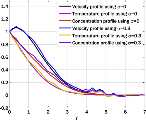
Figure 1. Comparison of the fractal and fractal stochastic models using $\alpha =0.5,\beta =3,{\lambda }_1=1,{\lambda }_2=0.7,\mathit{Pr}=1,Rd=0.1,Q=0.1,Nb=0.1,Nt=0.1,Sc=1,\gamma =0.1$

Figure 2 shows the comparison of existing and proposed numerical schemes. Upon examination of Figure 2, it becomes evident that the proposed scheme exhibits a higher convergence rate than the preexisting Crank-Nicolson scheme when applied to the fractal model. Figure 3 displays the Casson parameter’s effect on the fractal model’s velocity profile. The velocity profile decreases by incrementing the Casson parameter. The increment in the Casson parameter produces decay in the coefficient of diffusion term, and due to this decay of diffusion process in the fluid, the velocity of the fluid decays. This decay is due to the complex interaction between temperature gradient forces and fluid velocity.

Figure 2

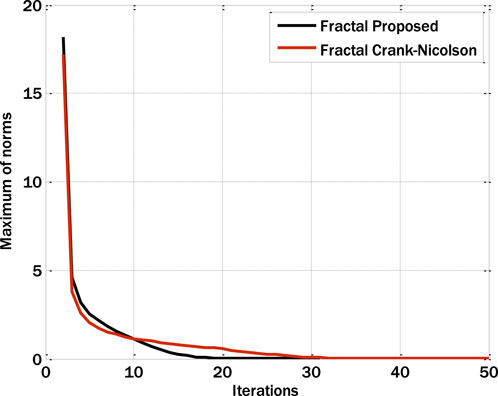
Figure 2. Comparison of the fractal proposed and fractal Crank-Nicolson schemes using $\alpha =0.5,\beta =3,{\lambda }_1=1,{\lambda }_2=0.7,\mathit{Pr}=1,Rd=0.1,Q=0.1,Nb=0.1,Nt=0.1,Sc=1,\gamma =0.1$

Figure 3

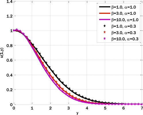
Figure 3. Effect of Casson parameter on velocity profile for the fractal model using ${\lambda }_1=0.5,{\lambda }_2=0.7,\mathit{Pr}=1,Rd=0.1,Q=0.1,Nb=0.1,Nt=0.1,Sc=1,\gamma =1,\sigma =0$

The effect of the thermal mixed convection parameter on the velocity profile is displayed in Figure 4. The velocity profile is enhanced by raising the thermal mixed convection parameter. The temperature gradient is one of the forces in the mixed convection flows that can be responsible for the rise and fall of the flow velocity. Due to the boundaries, the figures give an overwhelming response for the extended time, thus giving a detailed idea of how the features and the system operate.

Figure 4

Figure 4. Effect of thermal mixed convection parameter on velocity profile for the fractal model using $\beta =3,{\lambda }_2=0.7,\mathit{Pr}=1,Rd=0.1,Q=0.1,Nb=0.1,Nt=0.1,Sc=1,\gamma =1,\sigma =0$

Figure 5 shows the change in the temperature distribution profile due to the heating source parameter. Here, we can see that the profile’s temperature increases with an increment in the heating source parameter. Now, the fluid is being heated with radiation from a heat source. In other words, the heat flow of the fluid increases with the incident radiation power. Therefore, the temperature profile of the fluid graph is also increasing. Figure 6 shows the influence of radiation parameters on the temperature profile. As can be observed from the figure, the temperature profile of the fluid is facing an increasing trend due to the increase in radiation parameters. An increase in incoming radiation flux increases the heat flux, thus raising the temperature profile. Figure 7 shows the influence of the Brownian motion parameter on the temperature profile. The motion of the hot particles is now generally increasing the temperature profile of the fluid. The correlation between the temperature profile and the variation of the thermophoresis parameters is shown in Figure 8. As the values of the thermophoresis parameters rise, so does the temperature profile. Accelerating the thermophoresis parameter results in an enhanced rotational process whereby heated particles are transported more rapidly from the plate to the vicinity of the plate and vice versa. As a consequence of the progressive advancement of this cycle, particles with higher thermal energy migrate towards distinct regions within the fluid, resulting in an elevation of the fluid’s temperature.

Figure 5

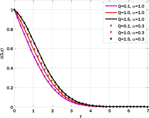
Figure 5. Effect of heat source parameter on a temperature profile for the fractal model using $\beta =3,{\lambda }_2=0.7,\mathit{Pr}=1,Rd=0.1,{\lambda }_1=1.0,Nb=0.1,Nt=0.1,Sc=1,\gamma =1,\sigma =0$

Figure 6

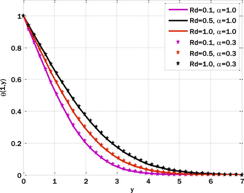
Figure 6. Effect of radiation parameter on a temperature profile for the fractal model using $\beta =3,{\lambda }_2=0.7,\mathit{Pr}=1,Q=0.1,{\lambda }_1=1.0,Nb=0.1,Nt=0.1,Sc=1,\gamma =1,\sigma =0$

Figure 7

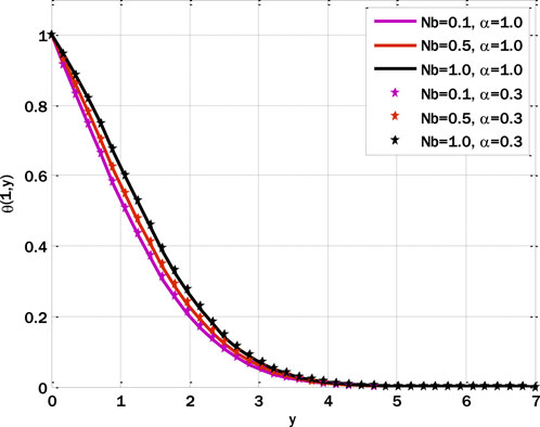
Figure 7. Effect of Brownian motion parameter on a temperature profile for the fractal model using $\beta =3,{\lambda }_2=0.7,\mathit{Pr}=1,Q=0.1,{\lambda }_1=1.0,Rd=0.1,Nt=0.1,Sc=1,\gamma =1,\sigma =0$

Figure 8

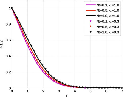
Figure 8. Effect of thermophoresis parameter on a temperature profile for the fractal model using $\beta =3,{\lambda }_2=0.7,\mathit{Pr}=1,Q=0.1,{\lambda }_1=1.0,Rd=0.1,Nb=0.1,Sc=1,\gamma =1,\sigma =0$

A correlation between the temperature profile and the variation of the Brownian motion parameter is seen in Figure 9. As the Brownian motion parameter is increased, the concentration profile decreases. Figure 10 shows the impact of the reaction rate parameter on the concentration profile. The concentration profile diminishes due to the augmentation of the response rate parameter. The growing reaction rate parameter enhances the conversion of one substance into another, and the concentration profile decays. Figures 11, 12 show the fractal stochastic velocity profile mesh plots and Figures 13, 14 displays the contour plots for fractal stochastic velocity profile for the case of flow over an oscillatory sheet using cosine boundary conditions. The effect of boundary conditions over a long time can be seen in mesh plots. The complete discussion shows that each figure’s detailed analysis clearly indicates the type of mixed convective nanofluid flow with fractal features. The numerical scheme we gave has proved effective, as we could validate the results with the help of these figures.

Figure 9

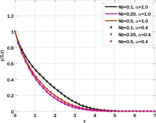
Figure 9. Effect of Brownian motion parameter on concentration profile for the fractal model using $\beta =3,{\lambda }_2=0.7,\mathit{Pr}=1,Q=0.1,{\lambda }_1=0.5,Rd=0.1,Nt=0.1,Sc=1,\gamma =1,\sigma =0$

Figure 10

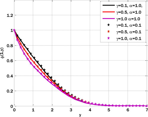
Figure 10. Effect of reaction rate parameter on concentration profile for the fractal model using $\beta =3,{\lambda }_2=0.7,\mathit{Pr}=1,Q=0.1,{\lambda }_1=0.5,Rd=0.1,Nt=0.1,Sc=1,Nb=0.1,\sigma =0$

Figure 11

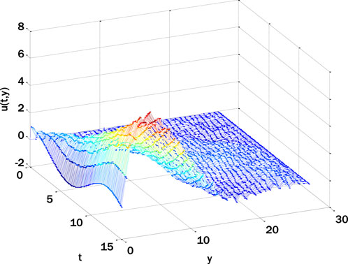
Figure 11. Mesh plot for fractal stochastic model using $\alpha =0.5,\beta =3,{\lambda }_2=0.5,\mathit{Pr}=1,Q=0.1,{\lambda }_1=1,Rd=0.1,Nt=0.1,Sc=1,\gamma =0.1,Nb=0.1,\sigma =0.3,u_0=\mathit{cos}\left(0.5t\right)$

Figure 12

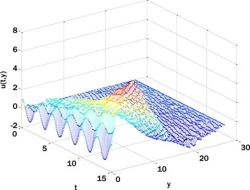
Figure 12. Mesh plot for fractal stochastic model using $\alpha =0.5,\beta =3,{\lambda }_2=0.5,\mathit{Pr}=1,Q=0.1,{\lambda }_1=1,Rd=0.1,Nt=0.1,Sc=1,\gamma =0.1,Nb=0.1,\sigma =0.3,u_0=\mathit{cos}\left(3t\right)$

Figure 13

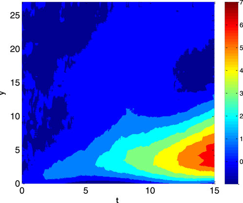
Figure 13. Contour plot for fractal stochastic model using $\alpha =0.5,\beta =3,{\lambda }_2=0.5,\mathit{Pr}=1,Q=0.1,{\lambda }_1=1,Rd=0.1,Nt=0.1,Sc=1,\gamma =0.1,Nb=0.1,\sigma =0.3,u_0=\mathit{cos}\left(0.5t\right)$

Figure 14

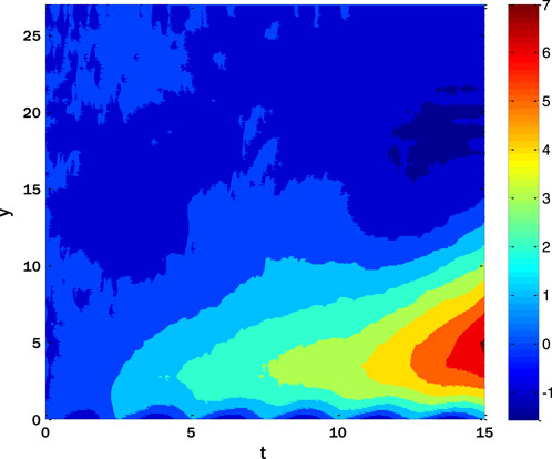
Figure 14. Contour plot for fractal stochastic model using $\alpha =0.5,\beta =3,{\lambda }_2=0.5,\mathit{Pr}=1,Q=0.1,{\lambda }_1=1,Rd=0.1,Nt=0.1,Sc=1,\gamma =0.1,Nb=0.1,\sigma =0.3,u_0=\mathit{cos}\left(3t\right)$

5 Conclusion

To better understand the fractal stochastic heat and mass transfer in mixed convective nanofluid flow, we propose a thorough numerical model in this work. The complex relationship between convective flow, nanofluid properties, and the randomness of heat and mass transfer within the system was effectively simulated and examined using the finite difference method. We suggest a finite difference scheme, a numerical technique for approximating derivatives in differential equations, to solve the equations numerically. The approach uses difference equations to approximatively calculate the spatial derivatives by discretizing the computational domain into a grid. Nanofluid flow behaviour can be simulated, thereby predicting heat and mass transfer characteristics. A two-dimensional mathematical model of such a boundary layer flow has been presented in this work. It is a time-dependent model that involves the flow over the plates. We introduced the mathematical heat and mass transfer model for boundary layer flow over the flat and oscillating sheets by considering the fractional time derivative. Nanofluids are fluids with nanoparticle suspensions, and their response under mixed convective conditions has been studied. The interaction between forced convection and natural convection is known as mixed convection. The temperature or concentration gradient condition produces natural convection in the fluid. Because of their unusual characteristics and interactions with the fluid, nanoparticles bring a new layer of complexity to the system. The proposed scheme has solved the problem, and the following concluding points are found,

i. The fractal scheme under consideration exhibited a higher convergence rate than the fractal Crank-Nicolson scheme.

ii. Increasing the Casson parameter in the fractal mathematical model causes the velocity profile to decay.

iii. The fractal model’s increasing heat source, thermal radiation, thermophoresis, and Brownian motion factors enhance the temperature profile.

iv. The concentration profile underwent decay due to the increasing values of the Brownian motion particle and the reaction rate parameter.

Our study highlights the significance of incorporating fractal stochastic heat and mass transport in the simulation of mixed convective nanofluid flows. Nanofluid properties’ elaborate and ever-changing nature and the influence of fractal stochastic phenomena create a multifaceted and dynamic system that opens up novel possibilities for scientific investigation and future technological progress. The present study establishes a fundamental basis for future inquiries and advancements in nanofluid dynamics and heat transfer.

Still, it is essential to discuss certain limitations of our work (Arif et al., 2023; Nawaz et al., 2024a; Nawaz et al., 2024b). Assumptions made based on the mathematical models might oversimplify the real-world scenarios. Although we took a numerical approach, future studies may need to elaborate on the models, keeping real-life scenarios in mind.

Data availability statement

The original contributions presented in the study are included in the article/supplementary material, further inquiries can be directed to the corresponding author.

Author contributions

MA: Conceptualization, Investigation, Supervision, Writing–original draft, Writing–review and editing. KA: Data curation, Formal Analysis, Funding acquisition, Resources, Visualization, Writing–review and editing. YN: Conceptualization, Investigation, Resources, Software, Writing–original draft.

Funding

The author(s) declare that no financial support was received for the research, authorship, and/or publication of this article. This research received no specific grant from the public, commercial, or not-for-profit funding agencies.

Acknowledgments

The authors wish to express their gratitude to Prince Sultan University for facilitating the publication of this article through the Theoretical and Applied Sciences Lab.

Conflict of interest

The authors declare that the research was conducted in the absence of any commercial or financial relationships that could be construed as a potential conflict of interest.

Publisher’s note

All claims expressed in this article are solely those of the authors and do not necessarily represent those of their affiliated organizations, or those of the publisher, the editors and the reviewers. Any product that may be evaluated in this article, or claim that may be made by its manufacturer, is not guaranteed or endorsed by the publisher.

References

Abbas, N., and Shatanawi, W. (2022). Heat and mass transfer of micropolar-casson nanofluid over vertical variable stretching riga sheet. Energies 15, 4945. doi:10.3390/en15144945

CrossRef Full Text | Google Scholar

Ahmad Sheikh, N., Ling Chuan Ching, D., Abdeljawad, T., Khan, I., Jamil, M., and Sooppy Nisar, K. (2021). A fractal-fractional model for the mhd flow of casson fluid in a channel. Comput. Mater. Continua 67 (2), 1385–1398. doi:10.32604/cmc.2021.011986

CrossRef Full Text | Google Scholar

Ali, A., Hussain, M., Anwar, M. S., and Inc, M. (2021a). Mathematical modeling and parametric investigation of blood flow through a stenosis artery. Appl. Math. Mech. 42, 1675–1684. doi:10.1007/s10483-021-2791-8

CrossRef Full Text | Google Scholar

Ali, I., Rasheed, A., Anwar, M. S., Irfan, M., and Hussain, Z. (2021b). Fractional calculus approach for the phase dynamics of Josephson junction. Chaos, Solit. Fractals 143, 110572. doi:10.1016/j.chaos.2020.110572

CrossRef Full Text | Google Scholar

Amjad, M., Zehra, I., Nadeem, S., Abbas, N., Saleem, A., and Issakhov, A. (2020). Influence of Lorentz force and induced magnetic field effects on Casson micropolar nanofluid flow over a permeable curved stretching/shrinking surface under the stagnation region. Surf. Interfaces 21, 100766. doi:10.1016/j.surfin.2020.100766

CrossRef Full Text | Google Scholar

Anwar, M. S. (2019). Modeling and numerical simulations of some fractional nonlinear viscoelastic flow problems (Lahore, Pakistan: Lahore University of Management of Science). PhD diss.

Anwar, M. S. (2020). Numerical study of transport phenomena in a nanofluid using fractional relaxation times in Buongiorno model. Phys. Scr. 95 (3), 035211. doi:10.1088/1402-4896/ab4ba9

CrossRef Full Text | Google Scholar

Anwar, M. S., Alam, M. M., Khan, M. A., Abouzied, A. S., Hussain, Z., and Puneeth, V. (2024). Generalized viscoelastic flow with thermal radiations and chemical reactions. Geoenergy Sci. Eng. 232, 212442. doi:10.1016/j.geoen.2023.212442

CrossRef Full Text | Google Scholar

Arif, M. S., Shatanawi, W., and Nawaz, Y. (2023). Modified finite element study for heat and mass transfer of electrical MHD non-Newtonian boundary layer nanofluid flow. Mathematics 11 (4), 1064. doi:10.3390/math11041064

CrossRef Full Text | Google Scholar

Babin, A. V., and Vishik, M. I. (1985). Attractors of Navier-Stokes systems and of parabolic equations, and estimates for their dimensions. J. Sov. Math. 28, 619–627. doi:10.1007/bf02112325

CrossRef Full Text | Google Scholar

Batra, R., and Jena, B. (1991). Flow of a Casson fluid in a slightly curved tube. Int. J. Eng. Sci. 29, 1245–1258. doi:10.1016/0020-7225(91)90028-2

CrossRef Full Text | Google Scholar

Bensoussan, A., and Teman, R. (1973). Équations stochastiques du type Navier–Stokes. J. Funct. Anal. 13, 195–222. doi:10.1016/0022-1236(73)90045-1

CrossRef Full Text | Google Scholar

Busnello, B. (1999). A probabilistic approach to the two-dimensional Navier-Stokes equations. Ann. Probab. 27, 1750–1780. doi:10.1214/aop/1022874814

CrossRef Full Text | Google Scholar

Casson, N. (1959). “A flow equation for pigment-oil suspensions of the printing ink type,” in Rheology of disperse systems (Oxford, UK: Pergamon Press).

Google Scholar

Chepyzhov, V. V., and Llyin, A. A. (2004). On the fractal dimension of invariant sets: applications to Navier–Stokes equation. Dis. Cont. Dyn. Syst. 10, 117–136. doi:10.3934/dcds.2004.10

CrossRef Full Text | Google Scholar

Cintosum, E., Smallwood, G. J., and Gulder, O. L. (2007). Flame surface fractal characteristics in premixed turbulent combustion at high turbulence intensities. AIAA J. 45, 2785–2789. doi:10.2514/1.29533

CrossRef Full Text | Google Scholar

Çolak, A. B., Shafiq, A., and Sindhu, T. N. (2022). Modeling of Darcy–Forchheimer bioconvective Powell Eyring nanofluid with artificial neural network. Chin. J. Phys. 77, 2435–2453. doi:10.1016/j.cjph.2022.04.004

CrossRef Full Text | Google Scholar

Constantin, P., Foias, C., Manley, O. P., and Temam, R. (1985). Determining modes and fractal dimension of turbulent flows. J. Fluid Mech. 150, 427–440. doi:10.1017/s0022112085000209

CrossRef Full Text | Google Scholar

Constantin, P., and Iyer, G. (2008). A stochastic Lagrangian representation of the three-dimensional incompressible Navier-Stokes equations. Commun. Pure Appl. Math. 61, 330–345. doi:10.1002/cpa.20192

CrossRef Full Text | Google Scholar

Crisan, D., Flandoli, F., and Holm, D. D. (2019). Solution properties of a 3D stochastic Euler Fluid equation. J. Nonlin. Sci. 29, 813–870. doi:10.1007/s00332-018-9506-6

CrossRef Full Text | Google Scholar

Das, B., and Batra, R. (1993). Secondary flow of a Casson fluid in a slightly curved tube. Int. J. Nonlinear Mech. 28, 567–577. doi:10.1016/0020-7462(93)90048-p

CrossRef Full Text | Google Scholar

Dash, R. K., Mehta, K. N., and Jayaraman, G. (1996). Casson fluid flow in a pipe filled with a homogeneous porous medi-um. Int. J. Eng. Sci. 34, 1145–1156. doi:10.1016/0020-7225(96)00012-2

CrossRef Full Text | Google Scholar

Eldabe, N. T., Saddeck, M. G., and El-Sayed, A. F. (2001). Heat transfer of MHD non-Newtonian Casson fluid flow between two rotating cylinders. Mech. Mech. Eng. 5, 237–251.

Google Scholar

Gangal, A. D., Parvate, A., and Satin, S. (2011). Calculus on fractal curves in rn. Fractals 19, 15–27. doi:10.1142/s0218348x1100518x

CrossRef Full Text | Google Scholar

Gawedzki, K. (2008). “Soluble models of turbulent transport,” in Non-equilibrium statistical mechanics and turbulence Editors S. Nazarenko, and O. Zaboronski 3 (Cambridge, UK: Cambridge Uniersity Press), 47–107.

Google Scholar

Gouldin, F. C. (1987). An application of fractals to modeling premixed turbulent flames. Comb. Flame 68, 249–266. doi:10.1016/0010-2180(87)90003-4

CrossRef Full Text | Google Scholar

Hinz, M., and Teplyaev, A. (2015). Local Dirichlet forms, Hodge theory, and the Navier–Stokes equations on topologically one-dimensional fractals. Trans. Amer. Math. Soc. 367, 1347–1380. doi:10.1090/s0002-9947-2014-06203-x

CrossRef Full Text | Google Scholar

Holm, D. D. (2015). Variational principles for stochastic fluid dynamics. Proc. R. Soc. A 471, 20140963. doi:10.1098/rspa.2014.0963

PubMed Abstract | CrossRef Full Text | Google Scholar

Hussain, M., Shoaib, M., Ranjha, Q. A., Anwar, M. S., Ahmad, Z., and Inc, M. (2023). Numerical solution to flow of Casson fluid via stretched permeable wedge with chemical reaction and mass transfer effects. Mod. Phys. Lett. B 38, 2341008. doi:10.1142/s0217984923410087

CrossRef Full Text | Google Scholar

Hussain, Z., Muhammad, S., and Anwar, M. S. (2021). Effects of first-order chemical reaction and melting heat on hybrid nanoliquid flow over a nonlinear stretched curved surface with shape factors. Adv. Mech. Eng. 13 (4), 168781402199952. doi:10.1177/1687814021999526

CrossRef Full Text | Google Scholar

Iqbal, M. S. (2011). Solutions of boundary value problems for nonlinear partial differential equations by fixed point methods.

Google Scholar

Khan, N. A., Ara, A., Ali, S. A., and Mahmood, A. (2009). Analytical study of Navier-Stokes equation with fractional orders using He's homotopy perturbation and variational iteration methods. Int. J. Nonlinear Sci. Numer. Simul. 10 (9), 1127–1134. doi:10.1515/ijnsns.2009.10.9.1127

CrossRef Full Text | Google Scholar

Kukavica, I. (2009). The fractal dimension of the singular set for solutions of the Navier–Stokes system. Nonlinearity 22, 2889–2900. doi:10.1088/0951-7715/22/12/005

CrossRef Full Text | Google Scholar

Kumar, D., Kumar, S., Abbasbandy, S., and Rashidi, M. M. (2014). Analytical solution of fractional Navier–Stokes equation by using modified Laplace decomposition method. Ain Shams Eng. J. 5, 569–574. doi:10.1016/j.asej.2013.11.004

CrossRef Full Text | Google Scholar

Lanjwani, H. B., Saleem, S., Chandio, M. S., Anwar, M. I., and Abbas, N. (2021). Stability analysis of triple solutions of Casson nanofluid past on a vertical exponentially stretching/shrinking sheet. Adv. Mech. Eng. 13, 168781402110596. doi:10.1177/16878140211059679

CrossRef Full Text | Google Scholar

Lanotte, A. S., Benzi, R., Malapaka, S. K., Toschi, F., and Biferale, L. (2015). Turbulence on a fractal Fourier set. Phys. Rev. Lett. 115, 264502. doi:10.1103/physrevlett.115.264502

PubMed Abstract | CrossRef Full Text | Google Scholar

Lanotte, A. S., Malapaka, S. K., and Biferale, L. (2016). On the vortex dynamics in fractal Fourier turbulence. Eur. Phys. J. E 39, 49. doi:10.1140/epje/i2016-16049-x

PubMed Abstract | CrossRef Full Text | Google Scholar

le Jan, Y., and Sznitman, A. S. (1997). Stochastic cascades and 3-dimensional Navier–Stokes equations. Probab. Theory Relat. Fields 109, 343–366. doi:10.1007/s004400050135

CrossRef Full Text | Google Scholar

Łukaszewicz, G., and Kalita, P. (2016). “Navier–Stokes Equations: an introduction with applications,” in Advances in mechanics and mathematics, vol. 34. Editors G. Łukaszewicz, and P. Kalita (Cham: Springer).

Google Scholar

Mahalov, A., Riti, E. S., and Leibovich, S. (1990). Invariant helical subspaces for the Navier-Stokes equations. Arch. Ration. Mech. Anal. 112, 193–222. doi:10.1007/bf00381234

CrossRef Full Text | Google Scholar

Marchioro, C., and Pulvirenti, M. (1984). “Vortex methods in two-dimensional fluid mechanics,” in Lecture notes in physics (Berlin Germany: Springer).

Google Scholar

Mazzi, B., and Vassilicos, J. C. (2004). Fractal-generated turbulence. J. Fluid Mech. 502, 65–87. doi:10.1017/s0022112003007249

CrossRef Full Text | Google Scholar

Nadeem, S., Haq, R. U., and Akbar, N. S. (2013). MHD three-dimensional boundary layer flow of Casson nanofluid past a linearly stretching sheet with convective boundary condition. IEEE Trans. Nanotechnol. 13, 109–115. doi:10.1109/tnano.2013.2293735

CrossRef Full Text | Google Scholar

Nawaz, Y., Arif, M. S., Abodayeh, K., Soori, A. H., and Javed, U. (2024b). A modification of explicit time integrator scheme for unsteady power-law nanofluid flow over the moving sheets. Front. Energy Res. 12, 1335642. doi:10.3389/fenrg.2024.1335642

CrossRef Full Text | Google Scholar

Nawaz, Y., Arif, M. S., Nazeer, A., Abbasi, J. N., and Abodayeh, K. (2024a). A two-stage reliable computational scheme for stochastic unsteady mixed convection flow of Casson nanofluid. Int. J. Numer. Methods Fluids. doi:10.1002/fld.5264

CrossRef Full Text | Google Scholar

Oyelakin, I. S., Mondal, S., and Sibanda, P. (2016). Unsteady Casson nanofluid flow over a stretching sheet with thermal radiation, convective and slip boundary conditions. Alex. Eng. J. 55, 1025–1035. doi:10.1016/j.aej.2016.03.003

CrossRef Full Text | Google Scholar

Palmer, T. N., and Williams, P. D. (2008). Introduction. Stochastic physics and climate modelling. Philos. Trans. R. Soc. A 366, 2419–2425. doi:10.1098/rsta.2008.0059

PubMed Abstract | CrossRef Full Text | Google Scholar

Parvate, A., and Gangal, A. D. (2009). Calculus on fractal subsets of real-line I: formulation. Fractals 17, 53–81. doi:10.1142/s0218348x09004181

CrossRef Full Text | Google Scholar

Parvate, A., and Gangal, A. D. (2011). Calculus on fractal subsets of real line II: conjugacy with ordinary calculus. Fractals 19, 271–290. doi:10.1142/s0218348x11005440

CrossRef Full Text | Google Scholar

Pishkoo, A., and Darus, M. (2021). Using fractal calculus to solve fractal Navier–Stokes equations, and simulation of laminar static mixing in COMSOL multiphysics. Frac. Fract. 5, 16. doi:10.3390/fractalfract5010016

CrossRef Full Text | Google Scholar

Pope, S. B. (1994). On the relationship between stochastic Lagrangian models of turbulence and second-moment closures. Phys. Fluids 6, 973–985. doi:10.1063/1.868329

CrossRef Full Text | Google Scholar

Rasheed, A., and Anwar, M. S. (2018). Numerical computations of fractional nonlinear Hartmann flow with revised heat flux model. Comput. Math. Appl. 76 (10), 2421–2433. doi:10.1016/j.camwa.2018.08.039

CrossRef Full Text | Google Scholar

Scheffer, V. (1978). Fractal geometry and turbulence-Navier-Stokes equations and the Hausdorff dimension. Acad. Sci. Paris Compt. Rend. A-Sci. Math. 282, 121.

Google Scholar

Shafiq, A., Çolak, A. B., and Sindhu, T. N. (2023). Modeling of Soret and Dufour's convective heat transfer in nanofluid flow through a moving needle with artificial neural network. Arabian J. Sci. Eng. 48 (3), 2807–2820. doi:10.1007/s13369-022-06945-9

CrossRef Full Text | Google Scholar

Shafiq, A., Çolak, A. B., Sindhu, T. N., and Muhammad, T. (2022). Optimization of Darcy-Forchheimer squeezing flow in nonlinear stratified fluid under convective conditions with artificial neural network. Heat Transf. Res. 53 (3), 67–89. doi:10.1615/heattransres.2021041018

CrossRef Full Text | Google Scholar

Shah, K., and Abdeljawad, T. (2024). Study of radioactive decay process of uranium atoms via fractals-fractional analysis. South Afr. J. Chem. Eng. 48, 63–70. doi:10.1016/j.sajce.2024.01.003

CrossRef Full Text | Google Scholar

Song, F., and Em Karniadakis, G. (2019). Fractional magnetohydrodynamics: algorithms and applications. J. Comp. Phys. 378, 44–62. doi:10.1016/j.jcp.2018.10.047

CrossRef Full Text | Google Scholar

Sreenivasan, K. R. (1991). Fractals and multifractals in fluid turbulence. Ann. Rev. Fluid Mech. 23, 539–600. doi:10.1146/annurev.fluid.23.1.539

CrossRef Full Text | Google Scholar

Sreenivasan, K. R., and Meneveau, C. (1986). The fractal facets of turbulence. J. Fluid Mech. 173, 357–386. doi:10.1017/s0022112086001209

CrossRef Full Text | Google Scholar

Srivastava, V., and Saxena, M. (1994). Two-layered model of Casson fluid flow through stenotic blood vessels: applications to the cardiovascular system. J. Biomech. 27, 921–928. doi:10.1016/0021-9290(94)90264-x

PubMed Abstract | CrossRef Full Text | Google Scholar

Ueki, Y., Tsuji, Y., and Nakamura, I. (1999). Fractal analysis of a circulating flow field with two different velocity laws. Eur. J. Mech. B/Fluids 18, 959–975. doi:10.1016/s0997-7546(99)00123-5

CrossRef Full Text | Google Scholar

Vishik, M. I., Komechi, A. I., and Fursikov, A. I. (1979). Some mathematical problems of statistical hydrodynamics. Russ. Math. Surv. 34, 149–234. doi:10.1070/rm1979v034n05abeh003906

CrossRef Full Text | Google Scholar

Wang, K., and Liu, S. (2016). Analytical study of time-fractional Navier–Stokes equation by using transform methods. Adv. Diff. Equa. 2016, 61. doi:10.1186/s13662-016-0783-9

CrossRef Full Text | Google Scholar

Yang, X.-G., Guo, B., and Li, D. (2020). The fractal dimension of pullback attractors for the 2D Navier–Stokes equations with delay. Math. Meth. Appl. Sci. 43, 9637–9653. doi:10.1002/mma.6634

CrossRef Full Text | Google Scholar

Zhang, X. (2012). Stochastic Lagrangian particle approach to fractal Navier–Stokes equations. Comm. Math. Phys. 311, 133–155. doi:10.1007/s00220-012-1414-2

CrossRef Full Text | Google Scholar