Application of improved graph convolutional networks in daily-ahead carbon emission prediction

With the increasing complexity of power systems and the proliferation of renewable energy sources, the task of calculating carbon emissions has become increasingly challenging. To address these challenges, we developed a new method for predicting carbon emission factors. Bayesian optimization technique graphical convolutional networks with long- and short-term network (BO-TGNN) is used to predict the carbon emissions of the power system. The method aims to quickly predict the day-ahead carbon emissions of power system nodes with enhanced feature extraction and optimized network training hyperparameters. The effectiveness of the proposed method is demonstrated through simulation tests on three different power systems using four deep learning algorithms. The method provides a tailored solution to the evolving needs of carbon reduction efforts and is a significant step forward in addressing the complexity of carbon emission calculations for modern power systems.

1 Introduction

Emission source analysis and emission trend prediction help electricity consumers (Zeng X. et al., 2023; Zhang X. et al., 2023) and power generation enterprises (Zhang et al., 2020; Ruhnau et al., 2022) explore effective paths and measures for carbon emission reduction and theoretically ensure the development of reasonable carbon reduction and emission reduction operations and behaviors (Sun and Huang, 2022). Therefore, there is a need to explore scientific methods to predict carbon emission. Considering the reduction of fossil fuels, replacing electricity with renewable energy is gradually becoming popular around the world, and the mechanisms between carbon footprint and other carbon reduction measures are worth exploring. In addition to renewable energy, the supply chain with hydrogen and ammonia is also favorable for shipping organizations and institutions (Yan et al., 2023).

For the carbon emission prediction, Gao et al. (2022) derived a differential formula-based gray prediction model with the whale optimization algorithm (WOA) for parameters’ optimization. The carbon emission forecast of the thermal power plant was analyzed in Zhou et al. (2017) with particle swarm optimization (PSO) for the parameter update of the backpropagation (BP) neural network. In Ye et al. (2023), the carbon emission of the industry zone was forecasted quickly via the combination of integrating autoregressive integrated moving average (ARIMA) and support vector regression (SVR). Another important part of the prediction area considering carbon emission is carbon emission peak (CEP) prediction (Gao et al., 2023). In Wu et al. (2018), stochastic impacts by regression on population, affluence, and technology (STIRPAT) is employed to predict the CEP for Qingdao, China. For the carbon emission reduction, Wu et al. (2022) adopted the radial basis function (RBF) neural network to extract the feature of the indices with the production of vinyl.

For the carbon emission price prediction, Yang et al. (2022) presented a generalized autoregressive conditional heteroscedasticity model to effectively obtain the price of the carbon, and a mixed-integer linear programming (MILP) model is constructed for the cooperation of the electricity market and carbon market. In Sun and Zhang (2022), a cooperation technique with least square support vector machine (LSSVM) and artificial fish swarm algorithm (AFSA) is constructed for the effective and robust of carbon price forecast. For the carbon emission factor (CEF) forecast, Sun and Huang (2022) adopted the machine learning technique, extreme learning machine (ELM), to learn the feature of CEF at a provincial level for carbon emissions in China, with a heuristic-based approach, WOA, for the optimal operation and fast convergence. For the prediction of carbon emission or CEF, Zhang X. et al. (2023) constructed a surrogated optimization with generalized regression neural network (GRNN) for the acceleration of a two-stage optimization model for the electricity vehicle. With the consumer satisfaction, the day-ahead optimization of air-conditioning control was conducted in Zeng X. et al. (2023) with a driving training-based optimization (DTBO).

With the continuous breakthroughs in artificial intelligence technology, deep learning algorithms with their efficient feature extraction and function approximation ability have gradually received more attention in the field of carbon emission-related prediction. Recurrent neural networks (RNNs) and their variants, including long short-term memory (LSTM) (Kong et al., 2019) and gated recurrent units (GRUs), focus on capturing the time dimension feature. Therefore, they are suitable for the task of time series prediction of carbon prices. The day-ahead prediction with time series of CEI was performed in Cai et al. (2023) based on the LSTM neural network. Later, in Chen et al. (2023), the real-time of CEI with 15 min data was evaluated with the gated cycle unit network. In Niu et al. (2022), the empirical mode decomposition (EMD) cooperated with dragonfly algorithm (DA) was employed to process the features of the time series data considering uncertainty. And four methods were performed for the simulation test of carbon price forecast. Zhang K. et al. (2023) formulated the feature decomposition and capture model for the carbon price via the cooperation of variational mode decomposition (VMD) and LSTM. The PSO is adopted to search the parameter of LSTM in Zeng Q. et al. (2023) for the CEP at Yangtze River Delta city cluster, China.

In addition, the graph convolutional neural network (GNN) is one of the brand-new areas of deep learning. It can capture non-Euclidean geometric spatial features of graph structures, such as traffic flow, metro lines, and chemical structures, more efficiently than traditional convolutional networks. Time series networks can effectively extract high-dimensional non-linear features between electricity quantities from massive historical time series data using gate structures and learn the non-linear relationships between carbon emission time series in the source network. Therefore, the graph convolution network with long- and short-term network (TGNN) is constructed for the carbon emission prediction. Recently, several studies have evaluated the applications of GNNs in power grids (Boyaci et al., 2022; Liu et al., 2022; Hansen et al., 2023; Liu et al., 2023). The Bayesian optimization utilizes Gaussian process regression to construct a selection function for obtaining the next sample point. This technique shows good competence for searching the hyperparameter of network in studies (De Baets et al., 2017; Aslam et al., 2021; Rana et al., 2021), such as load monitoring (Rana et al., 2021), cyber-attack detection (De Baets et al., 2017), and renewable energy power forecast (Aslam et al., 2021). Rana et al. (2021) combines Bayesian optimization with machine learning for non-invasive load monitoring. This process is repeated, including hyperparameter optimization and network parameter training. On account of these, this paper proposes a novel Bayesian optimal technique for the graph convolution network with long- and short-term network (BO-TGNN) for the prediction of carbon emissions in new power systems. Through the data-driven form, it can reduce the dependence on the grid topology and system parameters. With the addition of Bayesian optimization, the network’s hyperparameter optimization operation is carried out to improve the generalization and convergence ability of the data-driven model. Finally, the combination of the time series network can quickly predict the electrical quantity of the CEF forecast. There are three novel points in this research, which are explained below:

1) Different from Boyaci et al. (2022), Liu et al. (2022), Hansen et al. (2023), and Liu et al. (2023), the BO-TGNN algorithm can effectively extract the high-dimensional electrical quantity characteristics of the power system spatio-temporally, and it can predict these characteristics for the user nodes system by analyzing the historical data on the source–network–load parameter.

2) Consistent with De Baets et al. (2017), Aslam et al. (2021), and Rana et al. (2021), this method innovatively applies a spatio-temporal graph convolutional neural network based on Bayesian optimization to the power system network in order to rapidly and accurately predict the carbon emission factors of power system load nodes.

3) It can meet certain calculation accuracy requirements and show good ability to effectively adapt to the source–load dynamics of the power system, providing a powerful tool for sustainable monitoring and management of power system carbon emissions.

The rest of the paper is organized as follows: Section 2 introduces the mathematical model for the analysis for carbon emission factors. Section 3 gives the structure and detailed implementation of BO-TGNN. Simulation results and discussion with three power systems are presented in Section 4. At last, Section 5 summarizes the paper.

2 Mathematical model of the CEF calculation

For the carbon flow prediction based on the graph convolution network with a long- and short-term network, the prediction process is divided into five steps, as shown in Figure 1. It includes the load and generator historical series dataset, carbon emission factor computation and collection, network training, hyperparameter of networks based on the Bayesian optimization technique, and the day-ahead forecast application for the nodes or electricity consumers in power systems.

Figure 1

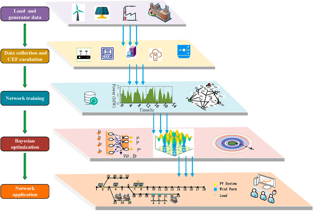
Figure 1. Framework of BO-TGNN for the power system and electricity consumer.

The first step is to collect the load historical sequence inputs from the PQ nodes, and Newton’s method is employed for power flow calculation. Then, the carbon flow analysis is performed and the load input data with the corresponding CEF output data on the power system nodes are collected. In the third step, the hyperparameters of the TGNN are selected as the variables for Bayesian optimization, followed by training the parameters of the network based on the collected data and updating the LSTM parameters by combining the loss function evaluation and backpropagation. In the fourth step, Bayesian optimization utilizes the Gaussian process regression to construct the ensemble function of the next sample point and repeats the hyperparameter optimization iterations and the training of the network parameters. Finally, the optimization is performed according to the real-time load sequence data and generator power output data, and the optimized optimal network is used for the online prediction of carbon emission coefficients to achieve a fast prediction of carbon emission coefficients at each node.

2.1 Calculation of the power flow

In order to predict day-ahead CEF, the primary task is to collect the historical load sequence inputs of PQ nodes and renewable energy power output data. Then, the power flow calculations should be performed. The power flow and voltage distribution of the power system are closely related. For containing $N_{\mathrm{g}}$ generators and $N_{\mathrm{n}}$ power bus, the power output of a power system with n nodes is divided into active and reactive parts. The power flow equation of the power system nodes can be expressed as follows:

$P_{\mathrm{G}}^i-P_{\mathrm{L}}^i=V_i{\displaystyle {\sum }_{j=1}^{N_{\mathrm{n}}}}{V}_j\left(G_{ij}\cos {\theta }_{ij}+B_{ij}\sin {\theta }_{ij}\right),(1)$

${\displaystyle {\sum }_{k=1}^{N_{\mathrm{g}}}}{Q}_{\mathrm{G}}^i-Q_{\mathrm{L}}^i=V_i{\displaystyle {\sum }_{j=1}^{N_{\mathrm{n}}}}{V}_j\left(G_{ij}\sin {\theta }_{ij}-B_{ij}\cos {\theta }_{ij}\right),(2)$

${\theta }_{ij}={\theta }_i-{\theta }_j,(3)$

$P_j^{\min }\le P_{\mathrm{G}}^i\le P_j^{\mathrm{m}\text{ax}},(4)$

$Q_j^{\min }\le Q_{\mathrm{G}}^i\le Q_j^{\mathrm{m}\text{ax}},(5)$

$V_j^{\min }\le V_j\le V_j^{\mathrm{m}\text{ax}},(6)$

where $P_{\mathrm{G}}^i$ and $P_{\mathrm{L}}^i$ are the active power values of the generator and load at node i, respectively; $Q_{\mathrm{G}}^i$ and $Q_{\mathrm{L}}^i$ are the reactive power values of the generator and load at node i, respectively; $G_{ij}$ and ${\mathrm{B}}_{\text{ij}}$ are the negative values of line i–j conductance and inductive reactance, respectively; $V_j$ denotes the voltage amplitudes at node i; ${\theta }_{ij}$ denotes the voltage angle difference between node i and node j; and ${\theta }_i$ denotes the voltage angle of node i, where $P_j^{\min }$, $P_j^{\mathrm{m}\text{ax}}$, $Q_j^{\min }$, $Q_j^{\mathrm{m}\text{ax}}$, $V_j^{\min }$, and $V_j^{\mathrm{m}\text{ax}}$ are the minimum and maximum values of active power regulation and reactive power regulation and output voltages for the jth generator, respectively.

2.2 Calculation of the carbon flow

In the carbon emission factor calculation, the CEF of the power system node corresponds to the active power of the input source and input source node. The calculation of CEF can be based on the above current results. The CEF equation can be expressed as follows:

${\delta }_{\mathrm{L},i}=\frac{P_{\mathrm{G}}^i\bullet {\delta }_{\mathrm{G},i}+{\displaystyle {\sum }_{j=1}^{N_{\mathrm{n}}}}{P}_{\mathrm{L}}^{i,j}\bullet {\delta }_{\mathrm{L},j}}{P_{\mathrm{G}}^i+{\displaystyle {\sum }_{j=1}^{N_{\mathrm{n}}}}{P}_{\mathrm{L}}^{i,j}},(7)$

$\left(P_{\mathrm{G}}^i+{\displaystyle {\sum }_{j=1}^{N_{\mathrm{n}}}}{P}_{\mathrm{L}}^{i,j}\right){\delta }_{\mathrm{L},i}-{\displaystyle {\sum }_{j=1}^{N_{\mathrm{n}}}}{P}_{\mathrm{L}}^{i,j}\bullet {\delta }_{\mathrm{L},j}=P_{\mathrm{G}}^i\bullet {\delta }_{\mathrm{G},i},(8)$

where ${\delta }_{\mathrm{L},i}$ $\left(i=1,2,\dots N_{\mathrm{n}}\right)$ is the set of solutions to the carbon flow equation, where $N_{\mathrm{n}}$ is the set of required solutions and equations. $\left(P_{\mathrm{G}}^i+{\displaystyle {\sum }_{j=1}^{N_{\mathrm{n}}}}{P}_{\mathrm{L}}^{i,j}\right)$ is the diagonal component of the carbon flow equation, which corresponds to the total power injected into the ith node; $P_{\mathrm{L}}^{i,j}$ is the active power injected along the line from the jth node to the ith node; and $P_{\mathrm{L}}^{i,j}$ is the non-diagonal component of the equation, which corresponds to the active power along the j–i line.

2.3 Construction of the data feature

The sequence data on the past ∆t length of the power system are selected as the input, which can be expressed as $\mathit{X}=\left\{{\mathit{X}}_1,{\mathit{X}}_2,\dots ,{\mathit{X}}_{T_{\mathrm{S}}-T_{\mathrm{h}}}\right\},\mathit{X}=\left\{{\mathit{x}}_1,{\mathit{x}}_2,\dots ,{\mathit{x}}_{T_{\mathrm{S}}-T_{\mathrm{h}}}\right\}.$ For a single moment, the network input feature quantity can be represented as ${\mathit{x}}_i=\left\{L_i,G_i,{\delta }_{\mathrm{L},i}\right\}\left(i=1,2,\dots ,T_{\mathrm{S}}-T_{\mathrm{h}}\right)$. $L=\left\{L_1,L_2,\dots ,L_{T_{\mathrm{S}}-T_{\mathrm{h}}}\right\}$, $=\left\{G_1,G_2,\dots ,G_{T_{\mathrm{S}}-T_{\mathrm{h}}}\right\}$, where $T_{\mathrm{S}}$ is the total collection data series length, $T_{\mathrm{h}}$ denotes the length of data series for a sample, and $T_{\mathrm{S}}-T_{\mathrm{h}}$ is the total valid number of collected samples. For the output characteristics of carbon emission factor trend analysis, it is necessary to consider the characteristic quantities of the output sequence of node carbon emission factors. Therefore, this article selects the load, new energy output, and carbon emission factor of each node as characteristic outputs. The network prediction feature quantity is the output of the network’s feature quantity at the next moment, which can be expressed as $\mathit{Y}=\left\{{\mathit{Y}}_1,{\mathit{Y}}_2,\dots ,{\mathit{Y}}_{T_{\mathrm{S}}-T_{\mathrm{h}}}\right\}$ and $Y_i=x_{i+T_{\mathrm{h}}}\left(i=1,2,\dots ,T_{\mathrm{S}}-T_{\mathrm{h}}\right)$.

3 Design of BO-TGNN for day-ahead CEF

The following flowchart in Figure 2 complements the specific steps of the BO-TGNN. In the upper part of the flowchart, the data source, calculation of electricity quantities, and data collection are presented for network training in the lower part of the flowchart. For GNN, the adjacency matrix should be determined according to the topology and line parameters of the power system. In the flowchart, network training and hyperparameter optimization are the cores of the whole prediction process. Bayesian optimization of the network hyperparameters involves a large loop of iterative Bayesian optimization. In each iteration of this grand loop, a series of network training iterations are performed.

Figure 2

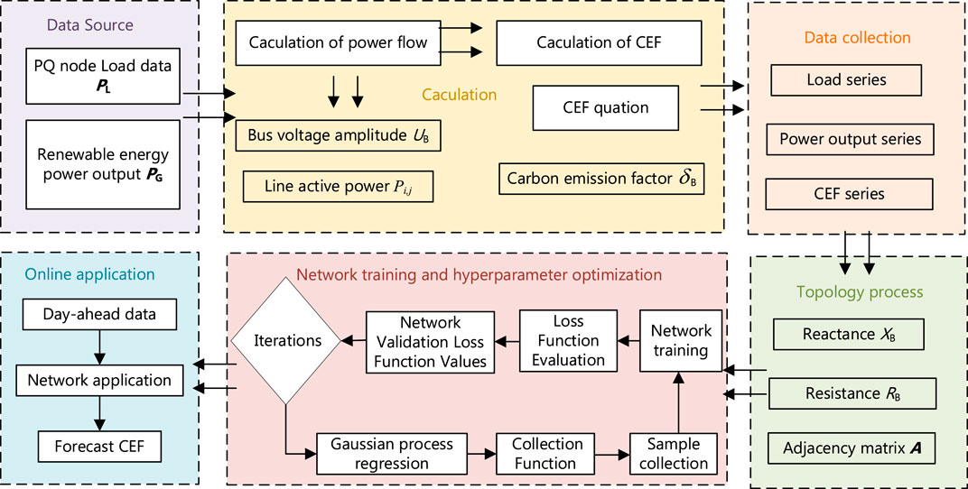
Figure 2. Flow diagram for the day-ahead CEF forecast with BO-TGNN.

3.1 Principle of LSTM

During the training of the network, historical sequences of input and output features of the dataset will be used to train the network parameters. The trained network will be utilized to quickly assess the carbon emission factors during the pre-testing process of the network. The forward propagation of LSTM with the gate and output computation is given as follows:

$\left\{\begin{array}{c}{f}_t=\sigma (w_f\bullet \left[\begin{array}{c}{h}_{t-1}\\ x_t\end{array}\right]+b_f\\ i_t=\sigma \left(w_i\bullet \left[\begin{array}{c}{h}_{t-1}\\ x_t\end{array}\right]+b_i\right)\\ g_t=\sigma \left(w_g\bullet \left[\begin{array}{c}{h}_{t-1}\\ x_t\end{array}\right]+b_g\right)\\ o_t=\sigma \left(w_o\bullet \left[\begin{array}{c}{h}_{t-1}\\ x_t\end{array}\right]+b_o\right),\end{array}\right.(9)$

where $x_t$ and $h_{t-1}$ denote the input of the tth time dimension; $f_{\mathrm{t}}$, $i_{\mathrm{t}}$, $g_{\mathrm{t}}$, and $o_{\mathrm{t}}$ are the forget, input state, new vector, and output state at the tth time dimension, respectively; $w_{\mathrm{f}}$, $w_{\mathrm{i}}$, $w_{\mathrm{g}}$, and $w_{\mathrm{o}}$, and $b_{\mathrm{f}}$, $b_{\mathrm{i}}$, $b_{\mathrm{g}}$, and $b_{\mathrm{o}}$ represent the weight and bias parameters of the LSTM layers, respectively; and $\left[\begin{array}{c}{\mathrm{h}}_{\mathrm{t}-1}\\ {\mathrm{x}}_{\mathrm{t}}\end{array}\right]$ represents the aggregation operation of two vectors.

3.2 Principle of GNN

GNN shows excellent performance in processing graph structured data. For a power system, it can represent graph relationships through topology and lines and use adjacency matrices to reflect the topological structure of the graph. In this paper, the topology of the power system and parameters of the lines (resistance $R_{\mathrm{B}}$ and reactance $X_{\mathrm{B}}$) are selected for the construction of adjacency matrix A, which are expressed as follows:

$\left\{\begin{array}{l}{\mathit{A}}_{ij}=\frac{{\overrightarrow{\mathit{v}}}_i-\min \overrightarrow{v}}{\max \overrightarrow{v}-\min \overrightarrow{v}}+\frac{{\overrightarrow{\mathit{u}}}_i-\min \overrightarrow{u}}{\max \overrightarrow{u}-\min \overrightarrow{u}}\\ {\overrightarrow{\mathit{v}}}_i=\frac{R_{i,j}-\underset{j=1,2,\dots N_n}{\mathrm{m}\text{in}}{R}_{i,j}}{\underset{j=1,2,\dots N_{\mathrm{n}}}{\max }{R}_{i,j}-\underset{j=1,2,\dots N_{\mathrm{n}}}{\mathrm{m}\text{in}}{R}_{i,j}}\\ {\overrightarrow{\mathit{u}}}_i=\frac{X_{i,j}-\underset{j=1,2,\dots N_n}{\mathrm{m}\text{in}}{X}_{i,j}}{\underset{j=1,2,\dots N_{\mathrm{n}}}{\max }{X}_{i,j}-\underset{j=1,2,\dots N_{\mathrm{n}}}{\mathrm{m}\text{in}}{X}_{i,j}}\end{array}\right.,(10)$

where ${\mathit{A}}_{ij}$ is the value of the adjacency matrix; ${\overrightarrow{\mathit{v}}}_i$ and ${\overrightarrow{\mathit{u}}}_i$ denote the elements of two normalized vectors; and $R_{i,j}$ and $X_{i,j}$ are the resistance and reactance between ith node and jth node.

Then, for the graph convolution operation of TGNN, the output feature can be determined by the adjacency matrix, input feature, and the optimal parameters, which is expressed as follows:

$\left\{\begin{array}{l}{H}_{\mathrm{c}}^{\text{out}}=\sigma \left({\stackrel{\sim }{D}}^{-\frac{1}{2}}\stackrel{\sim }{A}{\stackrel{\sim }{D}}^{-\frac{1}{2}}{H}_{\mathrm{c}}^{\text{in}}{w}_{\mathrm{c}}+b_{\mathrm{c}}\right),\\ \stackrel{\sim }{A}=A+I,\\ \stackrel{\sim }{D}={\sum }_{j=1}^{N_{\mathrm{n}}}{\stackrel{\sim }{A}}_{ij},\end{array}\right.(11)$

where $H_{\mathrm{c}}^{\text{out}}$ and $H_{\mathrm{c}}^{\text{in}}$ are the output and input features of the GNN layer, respectively; I denotes an identity matrix; $\stackrel{\sim }{D}$ is a degree matrix computed by $\stackrel{\sim }{A}$; and $w_{\mathrm{c}}$ and $b_{\mathrm{c}}$ are the parameters of the GNN.

3.3 Design of TGNN with Bayesian optimization

Due to good competence of LSTM for temporal feature extraction and GNN for spatial feature, the TGNN is employed to quickly forecast the carbon emission factor for power system and electricity consumers. The configuration of TGNN is given in Figure 3. It has four layers, including the input layer time series layer, graph convolution layer, and fully connected layer.

Figure 3

Figure 3. Network configuration of TGNN.

For hyperparameter optimization of TGNN, the Bayesian optimization technique is employed to search the optimum, which has three optimal steps. First, the hyperparameter of the system is determined by the sample operation for the current iterations, which is expressed as follows:

$f\left(\phi \right)\sim N[m\left(\phi \right),k\left(\phi ,{\phi }^{\prime }\right),(12)$

where $\phi$ is the optimal hyperparameter and $f\left(\phi \right)$ is the corresponding probability distribution function. ${\phi }_{\text{best}}$ is the location of the lowest posterior mean. $\omega \left({\phi }_{\text{best}}\right)$ is the minimum of the posterior mean.

Second, the forward propagation of the network is performed and the loss is calculated by the mean square error (MSE) function. Then, a collection function based on Gaussian process regression is constructed for collecting the sample set for the next iteration, which is expressed as follows:

$\overline{E}\left(\phi \right)=E\{\max \left[0,\omega \right.\left({\phi }_{\text{best}}\right)-f\left.\left.\left(\phi \right)\right]\right\},(13)$

where $\overline{E}\left(\phi \right)$ is the corresponding acquisition function.

Finally, the steps will be repeated until the iteration conditions are satisfied. The mean percentage error (MPE) function of the validation set is employed for the value evaluation, which is expressed as follows:

$\overline{\phi }=\arg \min e_{\text{mpe}}\left(\phi \right),\phi \in \overline{\mathit{\vartheta },}(14)$

where $\overline{\phi }$ is the optimal hyperparameter set, $\overline{\mathit{\vartheta }}$ denotes the optimal search space, and $e_{\text{mpe}}\left(\phi \right)$ is the objective function.

3.4 Calculation flow of BO-TGNN

The whole process of calculating the day-ahead CEF forecast by BO-TGNN is provided in the following Table 1. It follows three steps, namely, data collection, network training, and day-ahead application.

Table 1

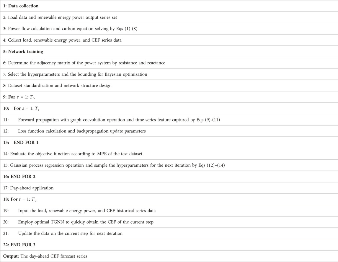
Table 1. Execution procedure of BO-TGNN for the day-ahead CEF forecast.

4 Case studies

In this paper, the IEEE-9 node, IEEE-39 node, and IEEE-118 node systems are employed to conduct simulation cases for simulation. In addition, the simulation is conducted with four algorithms, namely, BO-FULL, BO-LSTM, BO-GNN, and BO-TGNN. They all have the same hyperparameters and the same search space.

4.1 Dataset and parameters of three systems

The system topologies are shown in Figure 4A, Figure 5A, and Figure 6A. Then, the adjacency matrixes of the power systems for the GNN computation are given in Figure 4B, Figure 5B, and Figure 6B. These matrix values are determined by the topology, resistance, and reluctance of the power system nodes. The simulation uses 3 months of simulated data with a sampling time granularity of 15 min, considering the load fluctuation and renewable energy power output (as given in Figure 7). It has 11,520 sample data for deep learning technique training. The ratio of the training set to validation set is 1:4. The specific parameter data on the node system and algorithm are shown in Tables 2. For the carbon emission factor of the power system nodes, it related to the source end power generation technology of power system nodes. The renewable resources (like wind and PV) are set to 0 kg/kWh, the coal fired is set to 1.2 kg/kwh, and gas plant is set to 0.5 kg/kwh.

Figure 4

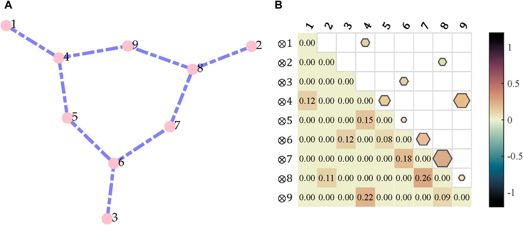
Figure 4. Spatial parameters of the IEEE-9 system. (A) Topology and (B) adjacency matrix.

Figure 5

Figure 5. Spatial parameters of the IEEE-39 system. (A) Topology and (B) adjacency matrix.

Figure 6

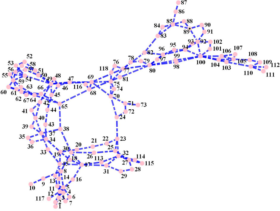
Figure 6. Spatial parameters of the IEEE-118 system. (A) Topology and (B) adjacency matrix.

Figure 7

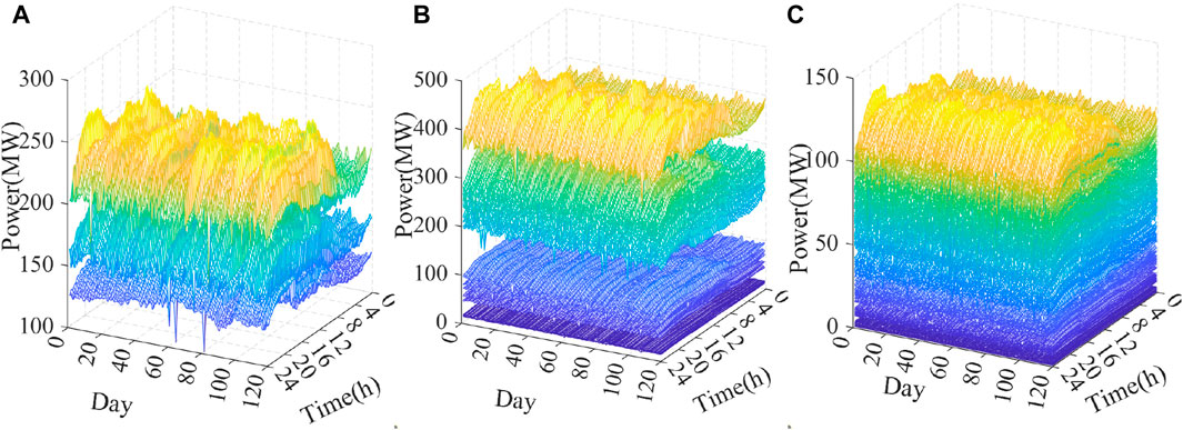
Figure 7. Fluctuation of the power system node considering the load and renewable power output. (A) IEEE-9, (B) IEEE-39, and (C) IEEE-118.

Table 2

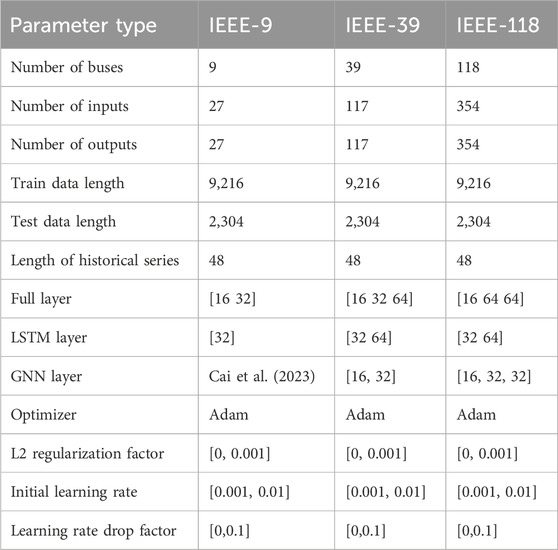
Table 2. System and algorithm parameter settings.

For Bayesian optimization, three hyperparameters of the four networks are selected, which are the L2 regularization factor, initial learning rate, and learning rate drop factor with the optimizer. These parameters are important for the network prediction performance, network training convergence, and generalization ability. To improve the transparency and understanding of the network for carbon emission factor prediction, these hyperparameters should be optimal reasonably. The iteration of Bayesian optimization is set to 35. The iteration of parameter optimization for deep learning is set to 100. The batch size of the training process is set to 64, and the Adam optimizer is selected for the network training. The time series length is set to 48 (12 h) for the day-ahead carbon emission factor forecast. The MPE is selected for the Bayesian optimization objective function, and MSE is selected for the network training loss function. MSE is widely used in regression models to analyze the prediction accuracy. MPE can better reflect the relative errors of various features in the model. For the mth dimension prediction result, the MPE and MSE can be given as follows:

$\text{MSE}=\frac{{\displaystyle {\sum }_{i=1}^m}{\left(y_i-{\overline{y}}_i\right)}^2}{m},(15)$

$\text{MPE}={\displaystyle {\sum }_{i=1}^m}\left|\frac{y_i-{\overline{y}}_i}{y_i}\right|.(16)$

4.2 Bayesian optimization for TGNN

Bayesian optimization is often applied to the hyperparameter optimization of networks, due to the good predictive performance requiring only a small number of iterations. It includes two iteration processes. The first iteration is the Bayesian optimization for hyperparameters for the network training, as shown in Figure 8A, Figure 9A, and Figure 10A. Then, the network parameters of the weight, bias parameters of each layer will be optimized according to the forward propagation and backward propagation, and the loss function of the convergence of the network will be obtained (as given in Figure 8B, Figure 9B, and Figure 10B).

Figure 8

Figure 8. Bayesian optimization results of the IEEE-9 system. (A) Bayesian optimization objective function and (B) MSE loss in network training for TGNN.

Figure 9

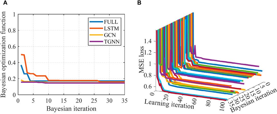
Figure 9. Bayesian optimization results of the IEEE-39 system. (A) Bayesian optimization objective function and (B) MSE loss in network training.

Figure 10

Figure 10. Bayesian optimization results of the IEEE-118 system. (A) Bayesian optimization objective function and (B) MSE loss in network training.

The following section discusses the optimal process of Bayesian optimization for each algorithm at different power systems. For the IEEE-9 node system, four algorithms eventually converge to approximate optimized values (as shown in Figure 8A). The TGNN converged first, followed by the GCN, LSTM, and FULL. The network training loss curves of TGNN for each Bayesian optimal iterations are given in Figure 8B.

In addition, for the IEEE-39 node system, the proposed TGNN has the best convergence value with the fastest convergence rate than the other three deep networks based on Bayesian optimization (as depicted in Figure 9A). In the network parameter training, Figure 9B shows the MSE loss function convergence process. With the vast majority of Bayesian optimization hyperparameters, the network parameter training converges at 30–40 iteration steps.

Finally, for the IEEE-118 node system, the best performance for Bayesian optimization can also be acquired with the cooperation of LSTM and GNN (as depicted in Figure 10A), and it has faster convergence rate and greater objective optimization than the IEEE-39 node system. This means that with the increase in power system’s nodes sizes, suitable network hyperparameter selection is necessary. This improves the predictive performance and convergence speed of the network. It is worth noting that the iterative loss function of the optimal hyperparameters in Figure 10B is instead higher than that of the other non-optimal iterative sets. This means that Bayesian optimization helps search the optimal hyperparameters and improve the generalization of the network, rather than simply improving the performance of the network’s loss function.

The Bayesian optimal parameter paths of the three systems with TGNN are given in Figure 11. For the IEEE-9 node system, the proposed Bayesian technique can optimize the parameters with a lower fluctuation (as depicted in Figure 9A). In the three parameters, the L2 regularization factor has the maximum numerical fluctuation than the other two parameters. In addition, parameter optimization fluctuations of the initial learning rate also gradually increased (as depicted in Figure 11B; Figure 11C). These indicate that Bayesian optimization can effectively explore the hyperparameters of the network.

Figure 11

Figure 11. Bayesian optimal parameters path with TGNN. (A) IEEE-9, (B) IEEE-39, and (C) IEEE-118.

4.3 Day-ahead optimization

4.3.1 Comparison for the power system node

The day-ahead results of CEFs for the power system node are given in Figure 12, Figure 13, and Figure 14 with prediction results of 3 days. For the IEEE-9 node system, the GCN shows shortcoming in predicting the carbon emission of the system due to the lack of the time series mechanism. The TGNN has the lower forecast error and fluctuation amplitude than the GCN (as shown in Figure 12). However, it fails to demonstrate advantages in comparing the performance of traditional algorithms, like FULL and LSTM. This may be due to the few features to the capture. In addition, in the IEEE-39 nodes system, it can track the trend of carbon emissions at nodes well. However, there are still lagging predictions at certain times, like 16:00 and 40:00. Finally, as given in Figure 13, the TGNN can track the fluctuation in carbon emission factors of power system nodes, indicating that it shows the best predictive performance on this testing system compared to other algorithms.

Figure 12

Figure 12. Day-ahead result of CEF in the IEEE-9 node system. (A) Node 9 and (B) node 7.

Figure 13

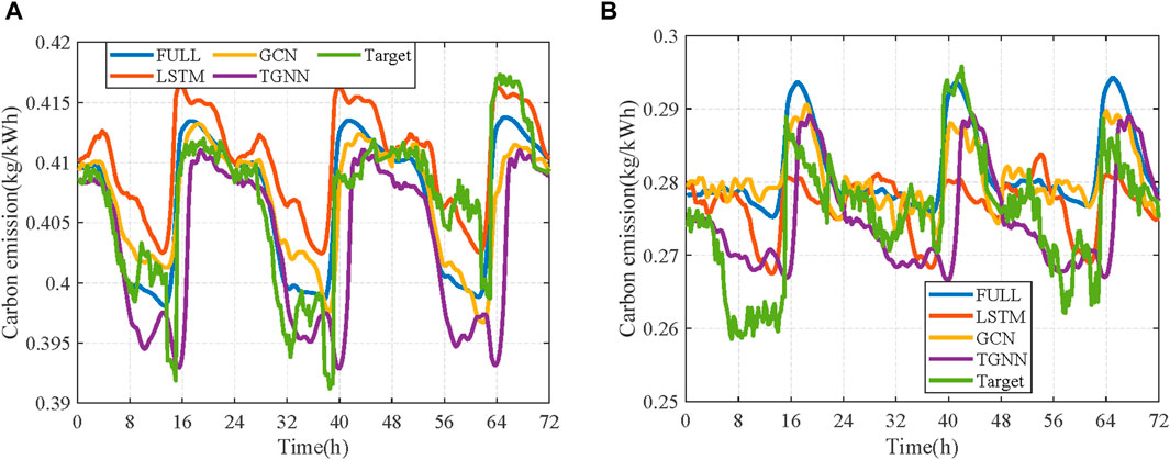
Figure 13. Day-ahead result of CEF for node 15 in the IEEE-39 node system. (A) Node 15 and (B) node 19.

Figure 14

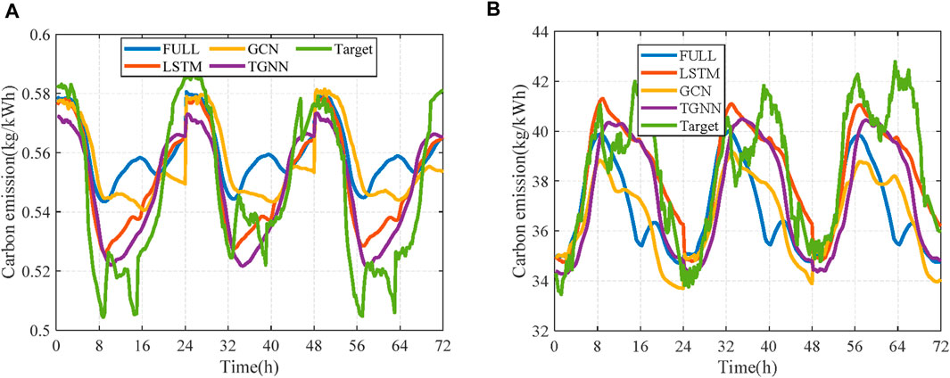
Figure 14. Day-ahead result of CEF for node 15 in the IEEE-118 node system. (A) Node 15 and (B) node 28.

4.3.2 Statistical results

To further evaluate the performance of the TGNN in the day-ahead CEF forecast, this section presents the application results of the four algorithms with three indexes separately, as shown in Table 3, where MSE is the loss function for deep network training. Higher values of MSE do not indicate a better network performance, and there may be network overfitting. In addition, MPE and the mean absolute error (MAE) are also used to evaluate the algorithm’s forward prediction performance. It is worth noting that the MPE function is also the objective function of Bayesian optimization. For the IEEE-9 node system, the MPE value is too terrible; this means that the network is hard to predict the results due to the bad hyperparameters for the network training. With the introduction of Bayesian optimization for hyperparameters of the deep network, the performance of the networks is improved. For the IEEE-39 node and 118 node systems, the proposed BO-TGNN has the lowest MPE; this means that it has the best performance for the prediction of the day-ahead carbon emission factor of the power system with larger node sizes. It can help improve the MPE performance for FULL with 89.3%, 53.3%, and 61.2%; LSTM with 94.9%, 67.9%, and 72.6%; GCN with 96.3%, 18.2%, and 86.7%; and TGNN with 98.9%, 7%, and 61.3%, respectively.

Table 3

Table 3. Result comparison with Bayesian optimization and none for each algorithm.

5 Conclusion

In conclusion, the work in this paper consists of the below two contributions:

1) The data-driven model is developed to effectively extract high-dimensional spatio-temporal electrical quantity characteristics of power systems, and these features of the user node system are predicted by analyzing the historical data on source–network–load parameters.

2) The method innovatively applies the spatio-temporal graph convolutional neural network based on Bayesian optimization to the power system network, which achieves a fast and accurate prediction of the daily-ahead carbon emission factor of a power system with a large node size.

In this paper, only the carbon emission factor is predictively analyzed and the impact of the response of the flexibility resources on the system is not considered. Future work will seriously address the uncertainty of wind and solar power generation in carbon emission prediction, in order to improve the comprehensiveness of prediction models. For the case of random changes in the load and new energy sources of the power system, the realistic resource response may not be consistent at all. In order to further improve the operation technology of the power system and power users, the carbon emission optimization model is subsequently considered to be combined with the forecasting technique to achieve the optimal carbon energy response of flexible loads.

Data availability statement

The raw data supporting the conclusion of this article will be made available by the authors, without undue reservation.

Author contributions

FP: conceptualization, funding acquisition, investigation, resources, writing–original draft, and writing–review and editing. YY: conceptualization, supervision, writing–original draft, and writing–review and editing. JL: funding acquisition, supervision, validation, and writing–original draft. JZ: data curation, formal analysis, resources, visualization, and writing–original draft. LZ: formal analysis, methodology, project administration, and writing–original draft. YJ: investigation, supervision, software, and writing–review and editing.

Funding

The author(s) declare that financial support was received for the research, authorship, and/or publication of this article. This work was jointly supported by the National Key Research and Development Program of China (2022YFF0606600) and the Science and Technology Project of China Southern Power Grid (GDKJXM20230256).

Conflict of interest

Authors FP, YY, YJ, JL, JZ, and LZ were employed by Metrology Center of Guangdong Power Grid Co., Ltd.

The authors declare that this study received funding from China Southern Power Grid. The funder had the following involvement in the study: Study design.

Publisher’s note

All claims expressed in this article are solely those of the authors and do not necessarily represent those of their affiliated organizations, or those of the publisher, the editors, and the reviewers. Any product that may be evaluated in this article, or claim that may be made by its manufacturer, is not guaranteed or endorsed by the publisher.

References

Aslam, M., Lee, S.-J., Khang, S.-H., and Hong, S. (2021). Two-stage attention over LSTM with bayesian optimization for day-ahead solar power forecasting. IEEE Access 9, 107387–107398. doi:10.1109/ACCESS.2021.3100105

CrossRef Full Text | Google Scholar

Boyaci, O., Umunnakwe, A., Sahu, A., Narimani, M. R., Ismail, M., Davis, K. R., et al. (2022). Graph neural networks based detection of stealth false data injection attacks in smart grids. IEEE Syst. J. 16, 2946–2957. doi:10.1109/JSYST.2021.3109082

CrossRef Full Text | Google Scholar

Cai, M., Huang, L., Zhang, Y., Liu, C., and Li, C. (2023). “Day-ahead forecast of carbon emission factor based on long and short-term memory networks,” in 2023 5th Asia Energy and Electrical Engineering Symposium (AEEES), Chengdu, China, 23-26 March 2023, 1568–1573. doi:10.1109/AEEES56888.2023.10114203

CrossRef Full Text | Google Scholar

Chen, S., Zheng, Y., Wen, X., Peng, Z., and Li, C. (2023). Research on real-time carbon emission factor prediction method for load nodes of power system based on gated recurrent cell network. 2023 3rd Power Syst. Green Energy Conf. (PSGEC), 683–688. doi:10.1109/PSGEC58411.2023.10256007

CrossRef Full Text | Google Scholar

De Baets, L., Ruyssinck, J., Develder, C., Dhaene, T., and Deschrijver, D. (2017). On the Bayesian optimization and robustness of event detection methods in NILM. Energy Build. 145, 57–66. doi:10.1016/j.enbuild.2017.03.061

CrossRef Full Text | Google Scholar

Gao, H., Wang, X., Wu, K., Zheng, Y., Wang, Q., Shi, W., et al. (2023). A review of building carbon emission accounting and prediction models. Buildings 13, 1617. doi:10.3390/buildings13071617

CrossRef Full Text | Google Scholar

Gao, M., Yang, H., Xiao, Q., and Goh, M. (2022). A novel method for carbon emission forecasting based on Gompertz’s law and fractional grey model: evidence from American industrial sector. Renew. Energy 181, 803–819. doi:10.1016/j.renene.2021.09.072

CrossRef Full Text | Google Scholar

Hansen, J. B., Anfinsen, S. N., and Bianchi, F. M. (2023). Power flow balancing with decentralized graph neural networks. IEEE Trans. Power Syst. 38, 2423–2433. doi:10.1109/TPWRS.2022.3195301

CrossRef Full Text | Google Scholar

Kong, W., Dong, Z. Y., Jia, Y., Hill, D. J., Xu, Y., and Zhang, Y. (2019). Short-term residential load forecasting based on LSTM recurrent neural network. IEEE Trans. Smart Grid 10, 841–851. doi:10.1109/TSG.2017.2753802

CrossRef Full Text | Google Scholar

Liu, S., Wu, C., and Zhu, H. (2022). Topology-aware graph neural networks for learning feasible and adaptive AC-OPF solutions. IEEE Trans. Power Syst. 38, 5660–5670. doi:10.1109/tpwrs.2022.3230555

CrossRef Full Text | Google Scholar

Liu, Y., Xie, H., Presekal, A., Stefanov, A., and Palensky, P. (2023). A GNN-based generative model for generating synthetic cyber-physical power system topology. IEEE Trans. Smart Grid 14, 4968–4971. doi:10.1109/TSG.2023.3304134

CrossRef Full Text | Google Scholar

Niu, X., Wang, J., Wei, D., and Zhang, L. (2022). A combined forecasting framework including point prediction and interval prediction for carbon emission trading prices. Renew. Energy 201, 46–59. doi:10.1016/j.renene.2022.10.027

CrossRef Full Text | Google Scholar

Rana, M. M., Bo, R., and Abdelhadi, A. (2021). Distributed grid state estimation under cyber attacks using optimal filter and bayesian approach. IEEE Syst. J. 15, 1970–1978. doi:10.1109/JSYST.2020.3010848

CrossRef Full Text | Google Scholar

Ruhnau, O., Bucksteeg, M., Ritter, D., Schmitz, R., Böttger, D., Koch, M., et al. (2022). Why electricity market models yield different results: carbon pricing in a model-comparison experiment. Renew. Sustain. Energy Rev. 153, 111701. doi:10.1016/j.rser.2021.111701

CrossRef Full Text | Google Scholar

Sun, W., and Huang, C. (2022). Predictions of carbon emission intensity based on factor analysis and an improved extreme learning machine from the perspective of carbon emission efficiency. J. Clean. Prod. 338, 130414. doi:10.1016/j.jclepro.2022.130414

CrossRef Full Text | Google Scholar

Sun, W., and Zhang, J. (2022). A novel carbon price prediction model based on optimized least square support vector machine combining characteristic-scale decomposition and phase space reconstruction. Energy 253, 124167. doi:10.1016/j.energy.2022.124167

CrossRef Full Text | Google Scholar

Wu, C. B., Huang, G. H., Xin, B. G., and Chen, J. K. (2018). Scenario analysis of carbon emissions’ anti-driving effect on Qingdao’s energy structure adjustment with an optimization model, Part Ⅰ: carbon emissions peak value prediction. J. Clean. Prod. 172, 466–474. doi:10.1016/j.jclepro.2017.10.216

CrossRef Full Text | Google Scholar

Wu, H., Han, Y., Geng, Z., Fan, J., and Xu, W. (2022). Production capacity assessment and carbon reduction of industrial processes based on novel radial basis function integrating multi-dimensional scaling. Sustain. Energy Technol. Assessments 49, 101734. doi:10.1016/j.seta.2021.101734

CrossRef Full Text | Google Scholar

Yan, X., He, Y., and Fan, A. (2023). Carbon footprint prediction considering the evolution of alternative fuels and cargo: a case study of Yangtze river ships. Renew. Sustain. Energy Rev. 173, 113068. doi:10.1016/j.rser.2022.113068

CrossRef Full Text | Google Scholar

Yang, Y., Liu, J., Xu, X., Xie, K., Lai, Z., Xue, Y., et al. (2022). Cooperative trading strategy of carbon emitting power generation units participating in carbon and electricity markets. Front. Energy Res. 10, 10. doi:10.3389/fenrg.2022.977509

CrossRef Full Text | Google Scholar

Ye, L., Du, P., and Wang, S. (2023). Industrial carbon emission forecasting considering external factors based on linear and machine learning models. J. Clean. Prod. 2023, 140010. doi:10.1016/j.jclepro.2023.140010

CrossRef Full Text | Google Scholar

Zeng, Q., Shi, C., Zhu, W., Zhi, J., and Na, X. (2023b). Sequential data-driven carbon peaking path simulation research of the Yangtze River Delta urban agglomeration based on semantic mining and heuristic algorithm optimization. Energy 285, 129415. doi:10.1016/j.energy.2023.129415

CrossRef Full Text | Google Scholar

Zeng, X., Zhang, Y., Guo, B., Huang, L., and Li, C. (2023a). “Optimal day-ahead dispatch of air-conditioning load under dynamic carbon emission factors,” in 2023 5th Asia Energy and Electrical Engineering Symposium (AEEES), Chengdu, China, 23-26 March 2023.

CrossRef Full Text | Google Scholar

Zhang, K., Yang, X., Wang, T., Thé, J., Tan, Z., and Yu, H. (2023b). Multi-step carbon price forecasting using a hybrid model based on multivariate decomposition strategy and deep learning algorithms. J. Clean. Prod. 405, 136959. doi:10.1016/j.jclepro.2023.136959

CrossRef Full Text | Google Scholar

Zhang, X., Gan, D., Wang, Y., Liu, Y., Ge, J., and Xie, R. (2020). The impact of price and revenue floors on carbon emission reduction investment by coal-fired power plants. Technol. Forecast. Soc. Change 154, 119961. doi:10.1016/j.techfore.2020.119961

CrossRef Full Text | Google Scholar

Zhang, X., Guo, Z., Pan, F., Yang, Y., and Li, C. (2023a). Dynamic carbon emission factor based interactive control of distribution network by a generalized regression neural network assisted optimization. Energy 283, 129132. doi:10.1016/j.energy.2023.129132

CrossRef Full Text | Google Scholar

Zhou, J., Du, S., Shi, J., and Guang, F. (2017). Carbon emissions scenario prediction of the thermal power industry in the beijing-tianjin-hebei region based on a back propagation neural network optimized by an improved particle swarm optimization algorithm. Pol. J. Environ. Stud. 26, 1895–1904. doi:10.15244/pjoes/68881

CrossRef Full Text | Google Scholar