Station-network cooperative planning method of urban integrated energy system based on energy flow model

Coordinated siting and sizing for energy stations and supply networks in urban integrated energy system (UIES) is significant for economic improvement and carbon emissions reduction. A station-network cooperative planning method of UIES based on energy flow model is proposed. First, an operation model of heat network based on energy flow theory is proposed, which solves the problem that the temperature mixing equation in the traditional operation model cannot be applied to heat network planning. On this basis, a bi-level model for station-network cooperative planning of UIES is constructed, in which the upper level optimizes the siting and sizing of the energy station and the topology of the supply network, and the lower level optimizes the operation of the UIES and feeds back the operation cost of the UIES to the upper level. Finally, a solution method of cooperative planning based on the Karush-Kuhn-Tucher condition is proposed, to transform the bi-level nonlinear optimization model into a single-level linear optimization model for efficient solution. Case studies on the 55-node and 77-road urban topology show that the proposed method can perform an effective planning on energy supply network topology and rationally configure the capacity of various devices in the energy station.

1 Introduction

With the continuous depletion of traditional fossil fuels and the increasingly serious problem of environmental pollution, there is an urgent need to form a new highly efficient, clean and sustainable way of utilizing multiple energy sources in a complementary manner (Strezoski et al., 2022). As an advanced energy utilization concept emerging in recent years, urban integrated energy system (UIES) can realize the coordinated complementary and efficient utilization of various types of energy sources, thereby increasing the rate of renewable energy consumption and reducing carbon emissions (Li et al., 2021). Therefore, it is of great significance to study the optimal configuration and operation optimization strategy of UIES under the background of dual carbon target (Chen et al., 2022).

Currently, global scholars have conducted a large number of studies on the planning of UIES. In Farrokhifar et al. (2020), a comprehensive summary of the planning research of UIES is provided from the perspectives of mathematical modeling, operation constraints, optimization objectives and methods of handling uncertainty. In Mu et al. (2020), a planning model for energy conversion and storage devices in UIES considering dynamic energy con-version efficiency coefficients is developed. In order to achieve carbon emission reduction, a device capacity planning strategy in UIES based on various device investment constraints is proposed in Wang et al. (2019). In Dong et al. (2023), an optimal expansion planning model for an integrated energy system consisting of a power grid, a gas network and multiple energy hubs is proposed. The references mentioned above focus on the planning problem of the capacity of the device in energy stations when the siting of the station and energy supply network are predetermined. However, the siting and sizing of the energy station and the energy supply network are interacting with each other, and the global optimal solution of UIES planning cannot be obtained when the siting of the station and the supply network are predetermined (Xiao et al., 2018). Therefore, further research is needed to investigate the cooperative planning of the siting and sizing of energy station with energy supply network.

In this context, a coordinated siting and sizing method for PIES that considers load complementary characteristics is proposed in Liu. (2020a). In Liu (2020b), an alternating optimization method based on cellular network theory is proposed for UIES’s energy station site selection, energy supply area division, and pipe network planning, and the Kruskal algorithm is used to determine the pipe network topology planning strategy. In Zhang et al. (2015), a long-term expansion planning methodology for energy hubs containing electric, gas and heat to optimally determine the least-cost planning schedules for generating units, transmission lines, gas boiler (GB) and combined heat and power (CHP) generation is proposed. However, these references do not use an exact model that includes variables such as thermal mass flow and temperature when modeling heat networks, but simply de-scribes them through thermal power balance constraints only, which will lead to inability to obtain accurate planning results.

To address this problem, a planning method of UIES consisting of a simulation model and an optimization model is proposed in Hong et al. (2018), where the simulation model adopts a two-layer bus structure, and considers both the energy flow in the external bus and the detailed network in the internal bus to achieve an accurate modeling of the thermal network in mass regulation mode. In Chen et al. (2024), a two-stage planning model of UIES for coordinating the location and size of the energy station as well as the supply net-work is proposed, where the optimal location of the energy station and the topology of the supply network are optimized to obtain the optimal location of the energy station in the first stage, and the size of the energy station and the pipeline network selection are optimized to obtain the optimal location of the energy station and the supply net-work topology in the second stage. However, all of the above references are planning with the topology of the heat network determined and does not consider planning for the heat supply pipeline. This is because the temperature mixing equation is only valid if the inlet and outlet of the heat pipeline are correctly determined, whereas the ther-mal mass flow direction cannot be predetermined when considering the planning of the heat pipeline, and therefore the model needs to be improved.

In this regard, by introducing an auxiliary heat variable and approximating the calculation equation of heat loss, the heat network model is transformed into a linear energy flow model in Xue et al. (2021), which can be applied to the planning problem of heat net-work to significantly improve the computational efficiency. Based on this model, for a mesh multi-energy distribution network (MMDN) containing electric, gas and heat, a resilience-oriented extended planning and reinforcement model is proposed in Li et al. (2023), to enhance the resilience of the MMDN through multi-energy coupling support, reinforcement, and reconfiguration strategies to resist low-probability high-damage un-foreseen events. In order to increase the penetration rate of wind power, a coordinated planning model for electric and heat based on the energy flow model and considering seasonal heat network reconfiguration is developed in Du et al. (2024), which is formulated as a mixed integer linear programming model. However, none of the energy flow-based heat network operation models in the above reference take into account the transmission delay characteristic of thermal mass, which cannot fully utilize the heat storage capacity of the heat network.

In summary, it can be seen that how to apply the energy flow model to the station-network cooperative planning of UIES and consider the transmission delay of thermal mass still needs to be investigated. Aiming at this problem, a station-network cooperative planning method of UIES based on energy flow model is proposed, which realizes the cooperative optimization of the siting and sizing of energy station and the topology of energy supply network. The main contributions are as follows:

(1) By introducing energy flow variables to replace the product of flow and temperature, and establishing the transmission delay characteristic equation, an energy flow-based heat network operation model is proposed, which solve the problem that the existing models do not take into account the transmission delay characteristic of thermal mass.

(2) A bi-level model for station-network cooperative planning of UIES is constructed, in which the upper level optimizes the siting and sizing of energy station and the topology of energy supply network with the objective of minimizing the total cost and passes it to the lower level, and the lower level optimizes the operation of the UIES according to the planning scheme and feeds back the total operation cost of the UIES to the upper level.

(3) A solution method of cooperative planning based on the Karush-Kuhn-Tucher (KKT) condition is proposed. Firstly, the nonlinear bi-level cooperative planning model is transformed into a bi-level linear model based on mathematical linearization theory to improve the solution efficiency, and then the bi-level linear model is transformed into a mixed-integer linear planning model which is easy to be solved based on the KKT condition.

The remainder is organized as follows. In Section 2, the operation model of heat network based on energy flow theory is proposed. In Section 3, the bi-level model for station-network cooperative planning of UIES is constructed. In Section 4, the solution method of cooperative planning based on the KKT condition is proposed. In Section 5, case studies are conducted to demonstrate the Effectiveness and efficiency of the proposed method. Conclusion is finally given in Section 6.

2 Operation model of heat network based on energy flow theory

2.1 Exact operation model of heat network

In the heat network, the return water is heated by the heat source, and enters the supply pipeline after the temperature rises, and is transmitted to each secondary heat exchanger station through the supply pipeline, and flows into the return pipeline again after heat exchange. The exact operation model of heat network is as follows (Wu et al., 2018; Ha et al., 2022):

$H_{i,t,s}^{\mathrm{N}}=c_{\mathrm{w}}{m}_i\left(T_{i,t,s}^{\mathrm{S}}-T_{i,t,s}^{\mathrm{R}}\right)(1)$

${\displaystyle \sum _{ki}}{m}_{ki}^{\mathrm{S}}={\displaystyle \sum _{ij}}{m}_{ij}^{\mathrm{S}}(2)$

${\displaystyle \sum _{ki}}{m}_{ki}^{\mathrm{R}}={\displaystyle \sum _{ij}}{m}_{ij}^{\mathrm{R}}(3)$

$T_{i,t,s}^{\mathrm{S}}{\displaystyle \sum _{ki}}{m}_{ki}^{\mathrm{S}}={\displaystyle \sum _{ki}}{m}_{ki}^{\mathrm{S}}{T}_{ki,t}^{\mathrm{S},\text{out}}(4)$

$T_{i,t,s}^{\mathrm{R}}{\displaystyle \sum _{ki}}{m}_{ki}^{\mathrm{R}}={\displaystyle \sum _{ki}}{m}_{ki}^{\mathrm{R}}{T}_{ki,t,s}^{\mathrm{R},\text{out}}(5)$

$T_{i,t,s}^{\mathrm{S}}=T_{ij,t,s}^{\mathrm{S},\text{in}}(6)$

$T_{i,t,s}^{\mathrm{R}}=T_{ij,t,s}^{\mathrm{R},\text{out}}(7)$

$T_{ij,t,s}^{\mathrm{S},\text{out}}=T_{t,s}^{\text{am}}+\left(T_{ij,t-{\tau }_{ij},s}^{\mathrm{S},\text{in}}-T_{t,s}^{\text{am}}\right)e^{-\frac{{\lambda }_{ij}{L}_{ij}}{m_{ij}^{\mathrm{S}}{A}_{ij}{\rho }_{\mathrm{w}}{c}_{\mathrm{w}}}}(8)$

$T_{ij,t,s}^{\mathrm{R},\text{out}}=T_{t,s}^{\text{am}}+\left(T_{ij,t-{\tau }_{ij},s}^{\mathrm{R},\text{in}}-T_{t,s}^{\text{am}}\right)e^{-\frac{{\lambda }_{ij}{L}_{ij}}{m_{ij}^{\mathrm{R}}{A}_{ij}{\rho }_{\mathrm{w}}{c}_{\mathrm{w}}}}(9)$

$T_{\min ,i}^{\mathrm{S}}\le T_{i,t,s}^{\mathrm{S}}\le T_{\max ,i}^{\mathrm{S}}(10)$

$T_{\min ,i}^{\mathrm{R}}\le T_{i,t,s}^{\mathrm{R}}\le T_{\max ,i}^{\mathrm{R}}(11)$

$m_{\min ,ij}^{\mathrm{S}}\le m_{ij}^{\mathrm{S}}\le m_{\max ,ij}^{\mathrm{S}}(12)$

$m_{\min ,ij}^{\mathrm{R}}\le m_{ij}^{\mathrm{R}}\le m_{\max ,ij}^{\mathrm{R}}(13)$

where H^N_i,t,s is the heat power of heat network node i at period t under scenario s; c_w is the specific heat capacity of water; m_i is the mass flow rate of heat exchanger at node i; T^S _i,t,s and T^R _i,t,s are the temperature of water flow at node i in supply/return network at period t under scenario s, respectively; m^S _ij and m^R _ij is the mass flow rate in pipe ij of supply and return networks, respectively; λ_ij is the thermal conductivity of pipe ij; L_ij is the length of the road between nodes i and j; A_ij is the cross-sectional area of pipe ij; ρ_w is the density of water; T^{S, in} _ij,t,s and $T_{\mathrm{ij},t,s}^{\text{R,in}}$ are the inlet temperatures of water flow in pipe ij of supply and return network at period t under scenario s, respectively; $T_{\mathrm{ij},\mathrm{t},\mathrm{s}}^{\text{S,out}}$ and $T_{\mathrm{ij},\mathrm{t},\mathrm{s}}^{\text{R,out}}$ are the outlet temperatures of water flow in pipeline ij of supply and return network at period t under scenario s, respectively; Tam t,s is the ambient temperature at period t under scenario s; τ_ij is the transmission delay of pipeline ij; T^S _max,i and T^S _min,i are the maximum and minimum temperatures of water in supply network for node i, respectively; $T_{\text{max},i}^{\text{R}}$ and $T_{\text{min},i}^{\text{R}}$ are the maximum and minimum temperatures of water in return network for node i, respectively; m^S _max,ij and $m_{\text{min},\mathit{ij}}^{\text{S}}$ are the maximum and minimum flow rates of the water in pipe ij of supply network, respectively; m^R _max,ij and m^R _min,ij are the maximum and minimum flow rates of the water in pipe ij of return network, respectively.

The above model cannot be directly applied to the station-network cooperative planning of UIES mainly because of the following two problems:

(1) In the exact operation model, the temperature mixing equations, i.e., Eqs. 4, 5, are only valid if the inlet and outlet of the heat pipe are correctly determined, whereas the direction of mass flow cannot be predetermined when considering the planning for heat network, and therefore the model cannot be used.

(2) The product term of mass flow rate and temperature exists in the exact model, which, if applied to the station-network cooperative planning of UIES, will make the planning model become a nonlinear optimization model, which not only has a poor solution efficiency, but may not be able to achieve the solution when the size of network is large.

Therefore, a heat network operation model based on theory (Xue et al., 2021) is constructed in this paper, which effectively solves the above two problems.

2.2 Energy flow-based heat network operation model

Based on the energy flow theory, utilizing an auxiliary variable instead of the nonlinear term (i.e., the product of temperature and mass flow rate) is considered in this paper, and defines the available heat quantity at the inlet and outlet of the pipe ij at period t under scenario s as hⁱⁿ _ij,t,s and h^out _ij,t,s, respectively, as shown in the following equation:

$h_{ij,t,s}^{\text{in}}=c_{\mathrm{w}}{m}_{ij}^{\mathrm{S}}\left(T_{ij,t,s}^{\mathrm{S},\text{in}}-T_{ij,t,s}^{\mathrm{R},\text{in}}\right)(14)$

$h_{ij,t,s}^{\text{out}}=c_{\mathrm{w}}{m}_{ij}^{\mathrm{S}}\left(T_{ij,t,s}^{\mathrm{S},\text{out}}-T_{ij,t,s}^{\mathrm{R},\text{out}}\right)(15)$

Then Eqs. 4, 5 are transformed into the following equation:

${\displaystyle \sum _{ki}}{h}_{ki,t,s}^{\text{out}}+H_{i,t,s}^{\mathrm{N}}={\displaystyle \sum _{ij}}{h}_{ij,t,s}^{\text{in}}(16)$

Due to the flow direction of heat pipeline in the UIES planning problem varies with the planning scheme, the energy flow-based heat network operation model in Xue et al. (2021) is unable to account for transmission delay characteristics of thermal mass. To address this issue, this paper depicts the flow direction of heat pipeline based on the spanning tree variables in the spanning tree theory, and rewrites the delay characteristic equation Eqs. 8, 9 into the following form:

$-\left(1-b_{ij}^{\mathrm{H}}\right)M\le h_{ij,t,s}^{\text{in}}-h_{ij,t-{\tau }_{ij},s}^{\text{out}}-h_{ij,t,s}^{\text{loss}}\le \left(1-b_{ij}^{\mathrm{H}}\right)M(17)$

$-\left(1-b_{ji}^{\mathrm{H}}\right)M\le h_{ij,t,s}^{\text{out}}-h_{ij,t-{\tau }_{ij},s}^{\text{in}}-h_{ij,t,s}^{\text{loss}}\le \left(1-b_{ji}^{\mathrm{H}}\right)M(18)$

$h_{ij,t,s}^{\text{loss}}=c_{\mathrm{w}}{m}_{ij}^{\mathrm{S}}\left(T_{ij,t,s}^{\mathrm{S},\text{in}}+T_{ij,t,s}^{\mathrm{R},\text{in}}-2T_{t,s}^{\text{am}}\right)\left(1-e^{-\frac{{\lambda }_{ij}{L}_{ij}}{m_{ij}^{\mathrm{S}}{A}_{ij}{\rho }_{\mathrm{w}}{c}_{\mathrm{w}}}}\right)(19)$

where $h_{\mathit{ij},\mathit{t},\mathit{s}}^{\text{loss}}$ is the loss of available heat quantity of the pipe ij at period t under scenario s; $b_{\mathit{ij}}^{\text{H}}$ and $b_{\mathit{ji}}^{\text{H}}$ are binary spanning tree variables. If node i is the parent of node j in the heat network, b^H _ij = 1 and b^H _ji = 0; if node j is the parent of node i, b^H _ji = 1 and b^H _ij = 0. When b^H _ij = 1, the flow direction of pipeline ij is from node i to node j, therefore Eq. 17 transform to $h_{ij,t,s}^{\text{in}}-h_{ij,t-{\tau }_{ij},s}^{\text{out}}-h_{ij,t,s}^{\text{loss}}=0$ to depict the transmission delay characteristic of the available heat quantity of the pipe ij. Eq. 18 is the same as Eq. 17.

Based on Eqs 10–13, the upper and lower constraints on the available heat quantity are respectively established as shown in Eqs 20–23 and give the calculation of the upper and lower limits of the available heat quantity.

$h_{\min ,ij}^{\text{in}}\le h_{ij,t,s}^{\text{in}}\le h_{\max ,ij}^{\text{in}}(20)$

$h_{\min ,ij}^{\text{out}}\le h_{ij,t,s}^{\text{out}}\le h_{\max ,ij}^{\text{out}}(21)$

$\left\{\begin{array}{l}{h}_{\max ,ij}^{\text{in}}=c_{\mathrm{w}}{m}_{\max ,ij}^{\mathrm{S}}\left(T_{\max }^{\mathrm{S}}-T_{\min }^{\mathrm{R}}\right)\\ h_{\max ,ij}^{\text{out}}=c_{\mathrm{w}}{m}_{\max ,ij}^{\mathrm{S}}\left(T_{\max }^{\mathrm{S}}-T_{\min }^{\mathrm{R}}\right)\end{array}\right.(22)$

$\left\{\begin{array}{l}{h}_{\min ,ij}^{\text{in}}=0\\ h_{\min ,ij}^{\text{out}}=0\end{array}\right.(23)$

where $h_{\text{max},\mathit{ij}}^{\text{in}}$ and $h_{\text{min},\mathit{ij}}^{\text{in}}$ are the upper and lower limits of the available heat quantity at the inlet of the pipe ij, respectively; h^out _{max, ij} and h^out _{min, ij} are the upper and lower limits of the available heat quantity at the outlet of the pipe ij, respectively; T^S _max and T^S _min are the maximum and minimum temperatures of water in supply network, respectively; T^R _max and T^R _min are the maximum and minimum temperatures of water in return network, respectively.

If the heat loss $h_{\mathit{ij},\mathit{t},\mathit{s}}^{\text{loss}}$ is determined, the operation model of heat network based on energy flow theory is independent of temperature and mass flow rate and can be solved directly without considering the direction of water flow. The nonlinear term λ_ijl_ij/$m_{ij}^{\mathrm{S}}{A}_{ij}{\rho }_{\mathrm{w}}{c}_{\mathrm{w}}$ in Eq. 19 is very close to 0, usually less than 0.001, so considering 1-e^-x≈x, the loss of available heat quantity can be approximated as (Dorfner and Hamacher, 2014):

$h_{ij,t,s}^{\text{loss}}\approx c_{\mathrm{w}}{m}_{ij}^{\mathrm{S}}\left(T_{ij,t,s}^{\mathrm{S},\text{in}}+T_{ij,t,s}^{\mathrm{R},\text{in}}-2T_{t,s}^{\text{am}}\right)\frac{{\lambda }_{ij}{L}_{ij}}{m_{ij}^{\mathrm{S}}{A}_{ij}{\rho }_{\mathrm{w}}{c}_{\mathrm{w}}}=\frac{{\lambda }_{ij}{L}_{ij}}{A_{ij}{\rho }_{\mathrm{w}}}\left(T_{ij,t,s}^{\mathrm{S},\text{in}}+T_{ij,t,s}^{\mathrm{R},\text{in}}-2T_{t,s}^{\text{am}}\right).(24)$

Since the only controllable variable affecting the loss of available heat quantity is temperature, the temperature of pipe should be kept lower to minimize the heat loss. In calculating the loss of available heat quantity, the inlet temperature of pipe in Eq. 21 is set as its lower limit, therefore:

$h_{ij,t,s}^{\text{loss}}=\frac{{\lambda }_{ij}{L}_{ij}}{A_{ij}{\rho }_{\mathrm{w}}}\left(T_{\min ,ij}^{\mathrm{S},\text{in}}+T_{\min ,ij}^{\mathrm{R},\text{in}}-2T_{t,s}^{\text{am}}\right)(25)$

where T^{S, in} _{min, ij} and T^{R, in} _{min, ij} are the lowest outlet temperatures of water flow in pipe ij of supply and return network, respectively.

3 Bi-level planning model of station-network cooperative optimization of UIES

3.1 Objective of the upper level planning model

The objective of the upper level is to minimize the total cost C^all, including the investment cost C^inv and the operation cost C^ope as shown in the following equation:

$\min C^{\text{all}}=C^{\text{inv}}+C^{\text{ope}}(26)$

The investment cost C^inv includes the device investment cost C^dv and the pipeline investment cost C^pl, as shown in the following equation:

$C^{\text{inv}}=C^{\text{line}}+C^{\text{device}}(27)$

$C^{\text{device}}={\displaystyle \sum _{i\in N^{\mathrm{P}}}}{\displaystyle \sum _{d\in {\mathrm{\Omega }}^{\mathrm{D}}}}{c}_{\text{inv}}^d{S}_i^d{R}_{\text{ir}}^d(28)$

$C^{\text{line}}={\displaystyle \sum _{ij\in L}}{\displaystyle \sum _{d\in {\mathrm{\Omega }}^{\mathrm{L}}}}{c}_{\text{inv}}^d{l}_{ij}{y}_{ij}^d{R}_{\text{ir}}^d(29)$

$R_{\text{ir}}^d=\frac{r{\left(1+r\right)}^{{\tau }^d}}{{\left(1+r\right)}^{{\tau }^d}-1}(30)$

where N^P is the set of candidate nodes of energy station; L is the set of roads; Ω^D is the set of the types of devices, including CHP, GB, electrical heater (EH), energy storage (ES), photovoltaic (PV) and wind turbine (WT); Ω^L is the set of the types of pipelines, including electric lines and heat pipes; cd inv is the investment cost factor for the d-category device/pipeline; R^d _ir is the payback factor for d-category device/pipeline, which spread the investment cost of the device over the planning period equally over the years of the life cycle; τ^d is the life of d-category devices/pipelines; S^d_i is the planning capacity of d-category device at node i; y^d _ij indicates whether d-category pipeline is installed between nodes i and j. If it is installed, y^d _ij,k = 1, otherwise, y^d_ij,k = 0.

3.2 Constraints of the upper level planning model

3.2.1 Constraints of planning for energy station

This paper considers that there are multiple candidate nodes of energy station, and defines the binary variable $y_i^S$ to indicate whether energy station is planned at node i. If it is planned, y^S _i = 1; otherwise, y^S _i = 0. The number of energy stations in the UIES needs to meet the following constraints:

$N_{\min }^{\mathrm{S}}\le {\displaystyle \sum _i}{y}_i^{\mathrm{S}}\le N_{\max }^{\mathrm{S}}(31)$

where N^S _min and N^S _max are the lower and upper limits of the number of energy stations, respectively.

The CHP units, GB, EH, ES, PV and WT can be configured only when the node is planning an energy station, so there:

$y_i^{\mathrm{S}}{S}_{\min ,i}^d\le S_i^d\le y_i^{\mathrm{S}}{S}_{\max ,i}^d,d\in \left\{\text{CHP},\text{GB},\text{EH},\text{ES},\text{WT},\text{PV}\right\}(32)$

where S^d_i denotes the installed capacity of d-category device at node i; S^d _min,i and S^d _max,i are the minimum and maximum installed capacity of d-category device at node i, respectively.

The total capacity of each type of equipment in the UIES needs to meet the following constraints:

$S_{\min }^d\le {\displaystyle \sum _i}{S}_i^d\le S_{\max }^d,d\in \left\{\text{CHP},\text{GB},\text{EH},\text{ES},\text{WT},\text{PV}\right\}(33)$

where S^d _min and S^d _max are the lower and upper limits of the total installed capacity of d-category equipment in the UIES.

3.2.2 Constraints of planning for energy supply network

In this paper, the planning of electric lines and heat pipes is considered, in order to ensure the radial structure of the electric network, the following constraints are in place. Eqs 31, 32 and give the calculation of the number of parent node of a node based on the spanning tree theory. Eq. 36 indicates that if a candidate node is planned as an energy station, it must be the root node and has no parent node. Eq. 37 indicates that each load node has a parent node. Eq. 38 indicates that nodes other than candidate nodes and load nodes have at most one parent node.

$y_{ij}^{\mathrm{E}}=b_{ij}^{\mathrm{E}}+b_{ji}^{\mathrm{E}}(34)$

$c_i^{\mathrm{E}}={\displaystyle \sum _{ji}}{b}_{ji}^{\mathrm{E}}(35)$

$c_i^{\mathrm{E}}\le 1-y_i^{\mathrm{S}},i\in N^{\mathrm{P}}(36)$

$c_i^{\mathrm{E}}=1,i\in N^{\mathrm{L}}(37)$

$c_i^{\mathrm{E}}\le 1,i\in N\backslash \left(N^{\mathrm{P}}\cup N^{\mathrm{L}}\right)(38)$

where N, N^P and N^L are the sets of all nodes, candidate energy station nodes and load nodes, respectively; y^E _ij indicates whether the electric line is planned between nodes i and j. If it is planned, y^E _ij = 1; otherwise, y^E _ij = 0; b^E _ij and b^E _ji are binary spanning tree variables. If node i is the parent of node j in the electric network, b^E _ij = 1 and b^E _ji = 0; if node j is the parent of node i, b^E _ji = 1 and b^E _ij = 0; c^E _i denotes the number of parent nodes of node i in the electric network.

Similarly, to ensure the radial structure of the heat network, the following constraints are imposed based on Eqs 34–38:

$y_{ij}^{\mathrm{H}}=b_{ij}^{\mathrm{H}}+b_{ji}^{\mathrm{H}}(39)$

$c_i^{\mathrm{H}}={\displaystyle \sum _{ji}}{b}_{ji}^{\mathrm{H}}(40)$

$c_i^{\mathrm{H}}\le 1-y_i^{\mathrm{S}},i\in N^{\mathrm{P}}(41)$

$c_i^{\mathrm{H}}=1,i\in N^{\mathrm{L}}(42)$

$c_i^{\mathrm{H}}\le 1,i\in N\backslash \left(N^{\mathrm{P}}\cup N^{\mathrm{L}}\right)(43)$

where y^H _ij indicates whether the heat pipe is planned between nodes i and j. If it is planned, $y_{\mathit{ij}}^{\text{H}}$ = 1; otherwise, $y_{\mathit{ij}}^{\text{H}}$ = 0; $c_{\mathit{i}}^{\text{H}}$ denotes the number of parent nodes of node i in the heat network.

3.3 Objective of the lower level planning model

The objective of the lower level is to minimize the operating cost C^ope, which includes purchasing electric cost $C_{\text{e}}^{\text{buy}}$, purchasing gas cost $C_{\text{g}}^{\text{buy}}$ and maintenance cost C^main, as shown in the following equation:

$\min C^{\text{ope}}=C_{\mathrm{e}}^{\text{buy}}+C_{\mathrm{g}}^{\text{buy}}+C^{\text{main}}(44)$

$C_{\mathrm{e}}^{\text{buy}}={\displaystyle \sum _s}{\displaystyle \sum _t}{\displaystyle \sum _i}{\alpha }_s^{\text{sce}}{P}_{i,t,s}^{\text{buy}}{c}_t^{\mathrm{E}}(45)$

$C_{\mathrm{g}}^{\text{buy}}={\displaystyle \sum _s}{\displaystyle \sum _t}{\displaystyle \sum _i}{\alpha }_s^{\text{sce}}{G}_{i,t,s}^{\text{buy}}{c}_t^{\mathrm{G}}(46)$

$C^{\text{main}}={\displaystyle \sum _{i\in N^{\mathrm{P}}}}{\displaystyle \sum _d}{c}_{\mathrm{m}}^d{S}_i^d+{\displaystyle \sum _{ij\in L}}{l}_{ij}\left(y_{ij}^{\mathrm{E}}{c}_{\mathrm{m}}^{\mathrm{E}}+y_{ij}^{\mathrm{H}}{c}_{\mathrm{m}}^{\mathrm{H}}\right)(47)$

where $P_{\mathit{i},\mathit{t},\mathit{s}}^{\text{buy}}$ is the power of purchasing electric at node i at period t under scenario s; $G_{\mathit{i},\mathit{t},\mathit{s}}^{\text{buy}}$ is the power of purchasing gas at node i at period t under scenario s; P^d _i,t,s is the output of d-category device at node i at period t under scenario s; $c_{\mathrm{m}}^{\mathit{d}}$ is the unit maintenance cost of d-category device; c^E _m and c^H _m are the unit maintenance cost of electric line and heat pipe, respectively.

3.4 Objective of the lower level planning model

3.4.1 Constraints of device

(1) Constraints of CHP.

The constraints of CHP are established as follows (Chen et al., 2023):

$H_{i,t,s}^{\text{CHP}}=K_{\mathrm{e}}^{\text{CHP}}{P}_{i,t,s}^{\text{CHP}}(48)$

$H_{i,t,s}^{\text{CHP}}=K_{\mathrm{h}}^{\text{CHP}}{G}_{i,t,s}^{\text{CHP}}(49)$

$P_{\min }^{\text{CHP}}{S}_i^{\text{CHP}}\le P_{i,t,s}^{\text{CHP}}\le P_{\max }^{\text{CHP}}{S}_i^{\text{CHP}}(50)$

$-r_{\max }^{\text{CHP}}{S}_i^{\text{CHP}}\Delta t\le P_{i,t,s}^{\text{CHP}}-P_{i,t-1,s}^{\text{CHP}}\le r_{\max }^{\text{CHP}}{S}_i^{\text{CHP}}\Delta t(51)$

where P^CHP _i,t,s, G^CHP _i,t,s and H^CHP _i,t,s are the electric power, gas consumption power and heat power of the CHP at node i at period t under scenario s, respectively; $K_{\mathrm{e}}^{\text{CHP}}$ is the heat-to-electric ratio coefficient of the CHP; $K_{\mathrm{h}}^{\text{CHP}}$ is the gas-heat conversion efficiency of the CHP; $P_{\text{max}}^{\text{CHP}}$ and $P_{\text{min}}^{\text{CHP}}$ are the upper and lower limits of the generation power of the CHP, respectively; $r_{\text{max}}^{\text{CHP}}$ is the maximum ramp rate of the CHP.

(2) Constraints of GB (Zhang et al., 2023).

$H_{i,t,s}^{\text{GB}}=K^{\text{GB}}{G}_{i,t,s}^{\text{GB}}(52)$

$H_{\min }^{\text{GB}}{S}_i^{\text{GB}}\le H_{i,t,s}^{\text{GB}}\le H_{\max }^{\text{GB}}{S}_i^{\text{GB}}(53)$

where $G_{\mathit{i},\mathit{t},\mathit{s}}^{\text{GB}}$ and H^GB _i,t,s are the gas consumption power and heat power of the GB at node i at period t under scenario s, respectively; K^GB is the heat-gas conversion factor of the GB; $H_{\text{max}}^{\text{GB}}$ and $H_{\text{min}}^{\text{GB}}$ are the upper and lower limits of the heat power of the GB, respectively.

(3) Constraints of EH (Chen et al., 2023).

$H_{i,t,s}^{\text{EH}}=K^{\text{EH}}{P}_{i,t,s}^{\text{EH}}(54)$

$H_{\min }^{\text{EH}}{S}_i^{\text{EH}}\le H_{i,t,s}^{\text{EH}}\le H_{\max }^{\text{EH}}{S}_i^{\text{EH}}(55)$

where P^EH _i,t,s and H^EH _i,t,s are electric power and heat power of the EH at node i at period t under scenario s, respectively; K^EH is the heat-electric conversion factor of the EH; HEH max and HEH min are the upper and lower limits of the heat power of the EH, respectively.

(4) Constraints of ES (Wang et al., 2021).

$x_{i,t,s}^{\text{ES},\mathrm{c}}+x_{i,t,s}^{\text{ES},\mathrm{f}}\le 1(56)$

$0\le P_{i,t,s}^{\text{ES},\mathrm{c}}\le x_{i,t,s}^{\text{ES},\mathrm{c}}{S}_i^{\text{ES}}(57)$

$0\le P_{i,t,s}^{\text{ES},\mathrm{f}}\le x_{i,t,s}^{\text{ES},\mathrm{f}}{S}_i^{\text{ES}}(58)$

$P_{i,t,s}^{\text{ES}}=P_{i,t,s}^{\text{ES},\mathrm{c}}-P_{i,t,s}^{\text{ES},\mathrm{f}}(59)$

$E_{i,t,s}^{\text{ES}}=E_{i,t-1,s}^{\text{ES}}+{\eta }^{\text{ES},\mathrm{c}}{P}_{i,t,s}^{\text{ES},\mathrm{c}}-\frac{P_{i,t,s}^{\text{ES},\mathrm{f}}}{{\eta }^{\text{ES},\mathrm{f}}}(60)$

$10\%E_i^{\text{ES},\mathrm{p}}\le E_{i,t,s}^{\text{ES}}\le 90\%E_i^{\text{ES},\mathrm{p}}(61)$

where x^ES,c _i,t,s and x^ES,f _i,t,s are the charging and discharging state of the ES at node i at period t under scenario s, respectively; P^ES,c _i,t,s and P^ES,f _i,t,s are the charging and discharging power of the ES at node i at period t under scenario s, respectively; E^ES _i,t,s is the capacity of the ES at node i at period t under scenario s; η^ES,c and η^ES,f are the charging and discharging efficiencies of the ES, respectively; $E_{\mathit{i}}^{\text{ES},\mathrm{p}}$ is the planning capacity of the ES at node i.

(5) Constraints of PV (Chen et al., 2023).

$0\le P_{i,t,s}^{\text{PV}}\le {\alpha }_{t,s}^{\text{PV},\text{pre}}{S}_i^{\text{PV}}(62)$

where ${\alpha }_{\mathit{t},\mathit{s}}^{\text{PV},\text{pre}}$ is the predicted output coefficients for PV at period t under scenario s; P^PV _i,t,s is the power outputs of PV at node i at period t under scenario s.

(6) Constraints of WT.

$0\le P_{i,t,s}^{\text{WT}}\le {\alpha }_{t,s}^{\text{WT},\text{pre}}{S}_i^{\text{WT}}(63)$

where ${\alpha }_{\mathit{t},\mathit{s}}^{\text{WT},\text{pre}}$ is the predicted output coefficients for WT at period t under scenario s; $P_{\mathit{i},\mathit{t},\mathit{s}}^{\text{WT}}$ is the power outputs of WT at node i at period t under scenario s.

(7) Constraints of Power of Purchasing Gas.

$G_{i,t,s}^{\text{buy}}=G_{i,t,s}^{\text{CHP}}+G_{i,t,s}^{\text{GB}}(64)$

3.4.2 Constraints of electric network

The power flow model of the electric network is established based on the LinDistFlow model as follows (Baran and Wu, 1989; Su et al., 2023):

$\left\{\begin{array}{l}{P}_{i,t,s}^{\mathrm{N}}=P_{i,t,s}^{\text{buy}}+P_{i,t,s}^{\text{CHP}}+P_{i,t,s}^{\text{PV}}+P_{i,t,s}^{\text{WT}}+P_{i,t,s}^{\text{ES}}-P_{i,t,s}^{\text{EH}}-P_{i,t,s}^{\text{load}}\\ Q_{i,t,s}^{\mathrm{N}}=Q_{i,t,s}^{\text{buy}}+Q_{i,t,s}^{\text{CHP}}+Q_{i,t,s}^{\text{PV}}+Q_{i,t,s}^{\text{WT}}-Q_{i,t,s}^{\text{EH}}-Q_{i,t,s}^{\text{load}}\end{array}\right.(65)$

$\left\{\begin{array}{l}{\displaystyle \sum _{ki\in L}}{P}_{ki,t,s}^{\mathrm{L}}+P_{i,t,s}^{\mathrm{N}}={\displaystyle \sum _{ij\in L}}{P}_{ij,t,s}^{\mathrm{L}}\\ {\displaystyle \sum _{ki\in L}}{Q}_{ki,t,s}^{\mathrm{L}}+Q_{i,t,s}^{\mathrm{N}}={\displaystyle \sum _{ij\in L}}{Q}_{ij,t,s}^{\mathrm{L}}\end{array}\right.(66)$

$-M\left(1-y_{ij}^{\mathrm{E}}\right)\le U_{i,t,s}^2-U_{j,t,s}^2-2P_{ij,t,s}^{\mathrm{L}}{R}_{ij}-2Q_{ij,t,s}^{\mathrm{L}}{X}_{ij}\le M\left(1-y_{ij}^{\mathrm{E}}\right)(67)$

$U_{\min }^2\le U_{i,t,s}^2\le U_{\max }^2(68)$

${\left(P_{ij,t,s}^{\mathrm{L}}\right)}^2+{\left(Q_{ij,t,s}^{\mathrm{L}}\right)}^2\le y_{ij}^{\mathrm{E}}{\left(S_{ij}\right)}^2(69)$

where P^N _i,t,s and Q^N _i,t,s are the active and reactive power at node i at period t under scenario s, respectively; P^L _ij,t,s and Q^L _ij,t,s are the active and reactive power transmitted by line ij at period t under scenario s, respectively; U² _i,t,s is the squared value of the voltage at node i at period t under scenario s; R_ij and X_ij are the resistance and reactance of line ij, respectively; M comes from the big-M method and is a sufficiently positive number, so that for any unplanned line ij, U² _i,t,s and U² _j,t,s do not directly influence each other; $U_{\mathit{\text{min}}}^2$ and $U_{\mathit{\text{max}}}^2$ are the squares of the lower and upper limits of voltage, respectively; S_ij is the capacity of line ij.

R_ij and X_ij in Eq. 67 require the substitutions shown in Eq. 70:

$\left\{\begin{array}{l}{R}_{ij}=y_{ij}^{\mathrm{E}}{l}_{ij}R\\ X_{ij}=y_{ij}^{\mathrm{E}}{l}_{ij}X\end{array}\right.(70)$

where R and X are the resistance and reactance per unit length of the electric line, respectively.

Then Eq. 67 is transformed into Eq. 71:

$-M\left(1-y_{ij}^{\mathrm{E}}\right)\le U_{i,t,s}^2-U_{j,t,s}^2-2P_{ij,t,s}^{\mathrm{L}}{y}_{ij}^{\mathrm{E}}{l}_{ij}R-2Q_{ij,t,s}^{\mathrm{L}}{y}_{ij}^{\mathrm{E}}{l}_{ij}X\le M\left(1-y_{ij}^{\mathrm{E}}\right)(71)$

3.4.3 Constraints of heat network

In addition to the energy flow-based heat network operation model developed in Section 2, the constraint shown in Eq. 72 is included.

$H_{i,t,s}^{\mathrm{N}}=H_{i,t,s}^{\text{CHP}}+H_{i,t,s}^{\text{GB}}+H_{i,t,s}^{\text{EH}}-H_{i,t,s}^{\text{load}}(72)$

In summary, the constraints of heat network include Eqs 16, 20, 21, 25, 72.

4 Solution method of station-network cooperative optimization of UIES

Firstly, the nonlinear terms in the cooperative optimization model are linearized based on mathematical theory, and the bi-level nonlinear optimization model is transformed into a bi-level linear optimization model. Then based on the Lagrangian function and KKT condition, the lower level model is transformed into the additional constraints of upper level model, and the bi-level linear optimization model is transformed into a single-level linear optimization model, which can be efficiently solved by commercial solvers.

4.1 Linearization of the cooperative planning model

The nonlinear terms P^L _{ij,t, syE ijlijR} and Q^L _{ij,t, syE ijlijR} appear in Eq. 71, which need to be linearized to improve the efficiency of the solution. Define the auxiliary variable Z^P _ij,t,s = P^L _ij,t,sy^E _ij, Z^Q _ij,t,s = Q^L _ij,t,sy^E _ij, where y^E _ij is a 0–1 variable, so there are the constraints shown in Eqs 73–76. When y^E _ij = 1, Eqs 73, 74 are translated into Z^P _ij,k,t,s = P^L _ij,t,s; when y^E _ij = 0, Eqs 73, 74 are translated into Z^P _ij,k,t,s = 0. Eqs 75, 76 are identical to the above.

$P_{ij,t,s}^{\mathrm{L}}-M\left(1-y_{ij}^{\mathrm{E}}\right)\le Z_{ij,t,s}^{\mathrm{P}}\le P_{ij,t,s}^{\mathrm{L}}+M\left(1-y_{ij}^{\mathrm{E}}\right)(73)$

$-M{y}_{ij}^{\mathrm{E}}\le Z_{ij,t,s}^{\mathrm{P}}\le M{y}_{ij}^{\mathrm{E}}(74)$

$Q_{ij,t,s}^{\mathrm{L}}-M\left(1-y_{ij}^{\mathrm{E}}\right)\le Z_{ij,t,s}^{\mathrm{Q}}\le Q_{ij,t,s}^{\mathrm{Q}}+M\left(1-y_{ij}^{\mathrm{E}}\right)(75)$

$-M{y}_{ij}^{\mathrm{E}}\le Z_{ij,t,s}^{\mathrm{Q}}\le M{y}_{ij}^{\mathrm{E}}(76)$

Then Eq. 71 is transformed into:

$-M\left(1-y_{ij}^{\mathrm{E}}\right)\le U_{i,t,s}^2-U_{j,t,s}^2-2Z_{ij,t,s}^{\mathrm{P}}{l}_{ij}R-2Z_{ij,t,s}^{\mathrm{Q}}{l}_{ij}X\le M\left(1-y_{ij}^{\mathrm{E}}\right).(77)$

Further, Eq. 69 is linearized based on quadratic constraint linearization method, and two square constraints Eq. 78 are employed to substitute for Eq. 69 (Chen et al., 2016).

$\left\{\begin{array}{l}-y_{ij}^{\mathrm{E}}{S}_{ij}\le P_{ij,t,s}^{\mathrm{L}}\le y_{ij}^{\mathrm{E}}{S}_{ij}\\ -y_{ij}^{\mathrm{E}}{S}_{ij}\le Q_{ij,t,s}^{\mathrm{L}}\le y_{ij}^{\mathrm{E}}{S}_{ij}\\ -\sqrt{2}{y}_{ij}^{\mathrm{E}}{S}_{ij}\le P_{ij,t,s}^{\mathrm{L}}+Q_{ij,t,s}^{\mathrm{L}}\le \sqrt{2}{y}_{ij}^{\mathrm{E}}{S}_{ij}\\ -\sqrt{2}{y}_{ij}^{\mathrm{E}}{S}_{ij}\le P_{ij,t,s}^{\mathrm{L}}-Q_{ij,t,s}^{\mathrm{L}}\le \sqrt{2}{y}_{ij}^{\mathrm{E}}{S}_{ij}\end{array}\right.(78)$

At this point, the bi-level nonlinear optimization model is transformed into a bi-level linear optimization model.

4.2 Transformation of the cooperative planning model based on KKT conditions

The Lagrangian function of the lower level model is shown in Eq. 79.

$L\left(q_u,q_l,\lambda ,\mu \right)=f\left(q_u,q_l\right)+{\displaystyle \sum _{i=1}^I}{\lambda }_i{b}_i\left(q_u,q_l\right)+{\displaystyle \sum _{j=1}^J}{\mu }_j{d}_j\left(q_u,q_l\right)(79)$

where f (q_u, q_l) is the objective function of the lower level model; b (q_u, q_l) and d (q_u, q_l) are the set of inequality constraints and the set of equation constraints of the lower level model, respectively; q_u and q_l are the decision variables of the upper level model and lower level model, respectively; λ_i∈λ and μ_j∈μ are the Lagrange multipliers of the inequality constraints and equation constraints in the lower level model, respectively; I and J are the number of inequality constraints and equation constraints in the lower level model, respectively.

Based on Eq. 79, the Lagrangian function of the lower level model is constructed as in Eq. 80.

$\begin{array}{l}{L}^{\text{LM}}={\displaystyle \sum _s}{\displaystyle \sum _t}{\displaystyle \sum _i}{\alpha }_s^{\text{sce}}{P}_{i,t,s}^{\text{buy}}{c}_t^{\mathrm{E}}+{\displaystyle \sum _s}{\displaystyle \sum _t}{\displaystyle \sum _i}{\alpha }_s^{\text{sce}}{G}_{i,t,s}^{\text{buy}}{c}_t^{\mathrm{G}}+{\displaystyle \sum _{i\in N^{\mathrm{P}}}}{\displaystyle \sum _d}{c}_{\mathrm{m}}^d{S}_i^d+{\displaystyle \sum _{ij\in L}}{l}_{ij}\left(y_{ij}^{\mathrm{E}}{c}_{\mathrm{m}}^{\mathrm{E}}+y_{ij}^{\mathrm{H}}{c}_{\mathrm{m}}^{\mathrm{H}}\right)+\\ {\lambda }_{i,t,s}^1\left(H_{i,t,s}^{\text{CHP}}-K_{\mathrm{e}}^{\text{CHP}}{P}_{i,t,s}^{\text{CHP}}\right)+{\lambda }_{i,t,s}^2\left(H_{i,t,s}^{\text{CHP}}-K_{\mathrm{h}}^{\text{CHP}}{G}_{i,t,s}^{\text{CHP}}\right)+{\lambda }_{i,t,s}^3\left(H_{i,t,s}^{\text{GB}}-K^{\text{GB}}{G}_{i,t,s}^{\text{GB}}\right)+\\ {\lambda }_{i,t,s}^4\left(H_{i,t,s}^{\text{EH}}-K^{\text{EH}}{P}_{i,t,s}^{\text{EH}}\right)+{\lambda }_{i,t,s}^5\left(P_{i,t,s}^{\text{ES}}-P_{i,t,s}^{\text{ES},\mathrm{c}}+P_{i,t,s}^{\text{ES},\mathrm{f}}\right)+{\lambda }_{i,t,s}^6\left(E_{i,t,s}^{\text{ES}}-E_{i,t-1,s}^{\text{ES}}-{\eta }^{\text{ES},\mathrm{c}}{P}_{i,t,s}^{\text{ES},\mathrm{c}}+P_{i,t,s}^{\text{ES},\mathrm{f}}/{\eta }^{\text{ES},\mathrm{f}}\right)+\\ {\lambda }_{i,t,s}^7\left(G_{i,t,s}^{\text{buy}}-G_{i,t,s}^{\text{CHP}}-G_{i,t,s}^{\text{GB}}\right)+{\lambda }_{i,t,s}^8\left(P_{i,t,s}^{\mathrm{N}}-P_{i,t,s}^{\text{buy}}-P_{i,t,s}^{\text{CHP}}-P_{i,t,s}^{\text{PV}}-P_{i,t,s}^{\text{WT}}-P_{i,t,s}^{\text{ES}}+P_{i,t,s}^{\text{EH}}+P_{i,t,s}^{\text{load}}\right)+\\ {\lambda }_{i,t,s}^9\left(Q_{i,t,s}^{\mathrm{N}}-Q_{i,t,s}^{\text{buy}}-Q_{i,t,s}^{\text{CHP}}-Q_{i,t,s}^{\text{PV}}-Q_{i,t,s}^{\text{WT}}+Q_{i,t,s}^{\text{EH}}+Q_{i,t,s}^{\text{load}}\right)+\\ {\lambda }_{i,t,s}^{10}\left({\displaystyle \sum _{ki\in L}}{P}_{ki,t,s}^{\mathrm{L}}+P_{i,t,s}^{\mathrm{N}}-{\displaystyle \sum _{ij\in L}}{P}_{ij,t,s}^{\mathrm{L}}\right)+{\lambda }_{i,t,s}^{11}\left({\displaystyle \sum _{ki\in L}}{Q}_{ki,t,s}^{\mathrm{L}}+Q_{i,t,s}^{\mathrm{N}}-{\displaystyle \sum _{ij\in L}}{Q}_{ij,t,s}^{\mathrm{L}}\right)+{\lambda }_{i,t,s}^{12}\left({\displaystyle \sum _{ki}}{h}_{ki,t,s}^{\text{out}}+H_{i,t,s}^{\mathrm{N}}-{\displaystyle \sum _{ij}}{h}_{ij,t,s}^{\text{in}}\right)+\\ {\lambda }_{i,t,s}^{13}\left(H_{i,t,s}^{\mathrm{N}}-H_{i,t,s}^{\text{CHP}}-H_{i,t,s}^{\text{GP}}-H_{i,t,s}^{\text{EH}}-H_{i,t,s}^{\text{load}}\right)+u_{i,t,s}^{1,\min }\left(P_{\min }^{\text{CHP}}{S}_i^{\text{CHP}}-P_{i,t,s}^{\text{CHP}}\right)+u_{i,t,s}^{1,\max }\left(P_{i,t,s}^{\text{CHP}}-P_{\max }^{\text{CHP}}{S}_i^{\text{CHP}}\right)+\\ u_{i,t,s}^{2,\min }\left(-r_{\max }^{\text{CHP}}{S}_i^{\text{CHP}}\Delta t-P_{i,t,s}^{\text{CHP}}+P_{i,t-1,s}^{\text{CHP}}\right)+u_{i,t,s}^{2,\max }\left(P_{i,t,s}^{\text{CHP}}-P_{i,t-1,s}^{\text{CHP}}-r_{\max }^{\text{CHP}}{S}_i^{\text{CHP}}\Delta t\right)+\\ u_{i,t,s}^{3,\min }\left(H_{\min }^{\text{GB}}{S}_i^{\text{GB}}-H_{i,t,s}^{\text{GB}}\right)+u_{i,t,s}^{3,\max }\left(H_{i,t,s}^{\text{GB}}-H_{\max }^{\text{GB}}{S}_i^{\text{GB}}\right)+u_{i,t,s}^{4,\min }\left(H_{\min }^{\text{EH}}{S}_i^{\text{EH}}-H_{i,t,s}^{\text{HP}}\right)+u_{i,t,s}^{4,\max }\left(H_{i,t,s}^{\text{EH}}-H_{\max }^{\text{EH}}{S}_i^{\text{EH}}\right)-\\ u_{i,t,s}^{5,\min }\left(x_{i,t,s}^{\text{ES},\mathrm{c}}+x_{i,t,s}^{\text{ES},\mathrm{f}}\right)+u_{i,t,s}^{5,\max }\left(x_{i,t,s}^{\text{ES},\mathrm{c}}+x_{i,t,s}^{\text{ES},\mathrm{f}}-1\right)-u_{i,t,s}^{6,\min }{P}_{i,t,s}^{\text{ES},\mathrm{c}}+u_{i,t,s}^{6,\max }\left(P_{i,t,s}^{\text{ES},\mathrm{c}}-x_{i,t,s}^{\text{ES},\mathrm{c}}{S}_i^{\text{ES}}\right)-\\ u_{i,t,s}^{7,\min }{P}_{i,t,s}^{\text{ES},\mathrm{f}}+u_{i,t,s}^{7,\max }\left(P_{i,t,s}^{\text{ES},\mathrm{f}}-x_{i,t,s}^{\text{ES},\mathrm{f}}{S}_i^{\text{ES}}\right)+u_{i,t,s}^{8,\min }\left(10\%E_i^{\text{ES},\mathrm{p}}-E_{i,t,s}^{\text{ES}}\right)+u_{i,t,s}^{8,\max }\left(E_{i,t,s}^{\text{ES}}-90\%E_i^{\text{ES},\mathrm{p}}\right)-\\ u_{i,t,s}^{9,\min }{P}_{i,t,s}^{\text{PV}}+u_{i,t,s}^{9,\max }\left(P_{i,t,s}^{\text{PV}}-{\alpha }_{t,s}^{\text{PV},\text{pre}}{S}_i^{\text{PV}}\right)-u_{i,t,s}^{10,\min }{P}_{i,t,s}^{\text{WT}}+u_{i,t,s}^{10,\max }\left(P_{i,t,s}^{\text{WT}}-{\alpha }_{t,s}^{\text{WT},\text{pre}}{S}_i^{\text{WT}}\right)+\\ u_{ij,t,s}^{11,\min }\left[-M\left(1-y_{ij}^{\mathrm{E}}\right)-U_{i,t,s}^2+U_{j,t,s}^2+2Z_{ij,t,s}^{\mathrm{P}}{l}_{ij}R+2Z_{ij,t,s}^{\mathrm{Q}}{l}_{ij}X\right]+\\ u_{ij,t,s}^{11,\max }\left[U_{i,t,s}^2-U_{j,t,s}^2-2Z_{ij,t,s}^{\mathrm{P}}{l}_{ij}R-2Z_{ij,t,s}^{\mathrm{Q}}{l}_{ij}X-M\left(1-y_{ij}^{\mathrm{E}}\right)\right]+\\ u_{ij,t,s}^{12,\min }\left[P_{ij,t,s}^{\mathrm{L}}-M\left(1-y_{ij}^{\mathrm{E}}\right)-Z_{ij,t,s}^{\mathrm{P}}\right]+u_{ij,t,s}^{12,\max }\left[Z_{ij,t,s}^{\mathrm{P}}-P_{ij,t,s}^{\mathrm{L}}-M\left(1-y_{ij}^{\mathrm{E}}\right)\right]+\\ u_{ij,t,s}^{13,\min }\left[Q_{ij,t,s}^{\mathrm{L}}-M\left(1-y_{ij}^{\mathrm{E}}\right)-Z_{ij,t,s}^{\mathrm{Q}}\right]+u_{ij,t,s}^{13,\max }\left[Z_{ij,t,s}^{\mathrm{Q}}-Q_{ij,t,s}^{\mathrm{Q}}-M\left(1-y_{ij}^{\mathrm{E}}\right)\right]+\\ u_{ij,t,s}^{14,\min }\left(-M{y}_{ij}^{\mathrm{E}}-Z_{ij,t,s}^{\mathrm{P}}\right)+u_{ij,t,s}^{14,\max }\left(Z_{ij,t,s}^{\mathrm{P}}-M{y}_{ij}^{\mathrm{E}}\right)+u_{ij,t,s}^{15,\min }\left(-M{y}_{ij}^{\mathrm{E}}-Z_{ij,t,s}^{\mathrm{Q}}\right)+u_{ij,t,s}^{15,\max }\left(Z_{ij,t,s}^{\mathrm{Q}}-M{y}_{ij}^{\mathrm{E}}\right)+\\ u_{ij,t,s}^{16,\min }\left(-y_{ij}^{\mathrm{E}}{S}_{ij}-P_{ij,t,s}^{\mathrm{L}}\right)+u_{ij,t,s}^{16,\max }\left(P_{ij,t,s}^{\mathrm{L}}-y_{ij}^{\mathrm{E}}{S}_{ij}\right)+u_{ij,t,s}^{17,\min }\left(-y_{ij}^{\mathrm{E}}{S}_{ij}-Q_{ij,t,s}^{\mathrm{L}}\right)+u_{ij,t,s}^{17,\max }\left(Q_{ij,t,s}^{\mathrm{L}}-y_{ij}^{\mathrm{E}}{S}_{ij}\right)+\\ u_{ij,t,s}^{18,\min }\left(-\sqrt{2}{y}_{ij}^{\mathrm{E}}{S}_{ij}-P_{ij,t,s}^{\mathrm{L}}-Q_{ij,t,s}^{\mathrm{L}}\right)+u_{ij,t,s}^{18,\max }\left(P_{ij,t,s}^{\mathrm{L}}+Q_{ij,t,s}^{\mathrm{L}}-\sqrt{2}{y}_{ij}^{\mathrm{E}}{S}_{ij}\right)+\\ u_{ij,t,s}^{19,\min }\left(-\sqrt{2}{y}_{ij}^{\mathrm{E}}{S}_{ij}-P_{ij,t,s}^{\mathrm{L}}+Q_{ij,t,s}^{\mathrm{L}}\right)+u_{ij,t,s}^{19,\max }\left(P_{ij,t,s}^{\mathrm{L}}-Q_{ij,t,s}^{\mathrm{L}}-\sqrt{2}{y}_{ij}^{\mathrm{E}}{S}_{ij}\right)+\\ u_{ij,t,s}^{20,\min }\left[-\left(1-b_{ij}^{\mathrm{H}}\right)M-h_{ij,t,s}^{\text{in}}+h_{ij,t-{\tau }_{ij},s}^{\text{out}}+h_{ij,t,s}^{\text{loss}}\right]+u_{ij,t,s}^{20,\max }\left[h_{ij,t,s}^{\text{in}}-h_{ij,t-{\tau }_{ij},s}^{\text{out}}-h_{ij,t,s}^{\text{loss}}-\left(1-b_{ij}^{\mathrm{H}}\right)M\right]+\\ u_{ij,t,s}^{21,\min }\left[-\left(1-b_{ji}^{\mathrm{H}}\right)M-h_{ij,t,s}^{\text{out}}+h_{ij,t-{\tau }_{ij},s}^{\text{in}}+h_{ij,t,s}^{\text{loss}}\right]+u_{ij,t,s}^{21,\max }\left[h_{ij,t,s}^{\text{out}}-h_{ij,t-{\tau }_{ij},s}^{\text{in}}-h_{ij,t,s}^{\text{loss}}-\left(1-b_{ji}^{\mathrm{H}}\right)M\right]+\\ u_{ij,t,s}^{22,\min }\left(h_{\min ,ij}^{\text{in}}-h_{ij,t,s}^{\text{in}}\right)+u_{ij,t,s}^{22,\max }\left(h_{ij,t,s}^{\text{in}}-h_{\max ,ij}^{\text{in}}\right)+u_{ij,t,s}^{23,\min }\left(h_{\min ,ij}^{\text{out}}-h_{ij,t,s}^{\text{out}}\right)+u_{ij,t,s}^{23,\max }\left(h_{ij,t,s}^{\text{out}}-h_{\max ,ij}^{\text{out}}\right)\end{array}(80)$

According to the constructed Lagrangian function and KKT complementary relaxation conditions, the lower level model can be transformed into the additional constraints of the upper level model, thus transforming the bi-level linear optimization model into a single-level linear optimization model, and the simplified form of the model is as follows:

$\underset{q_u\in Q_U,q_l\in Q_L}{\min }F\left(q_u,q_l\right)(81)$

$B\left(q_u,q_l\right)\le 0,D\left(q_u,q_l\right)=0(82)$

$b\left(q_u,q_l\right)\le 0,d\left(q_u,q_l\right)=0(83)$

${\nabla }_{q_l}L\left(q_u,q_l,\lambda ,\mu \right)=0(84)$

${\lambda }_i\ge 0,i=1,2,\dots ,I(85)$

${\lambda }_i{b}_i\left(q_u,q_l\right)=0,i=1,2,\dots ,I(86)$

where F (q_u, q_l) is the objective function of the upper level model; B (q_u, q_l) and D (q_u, q_l) are the set of inequality constraints and the set of equation constraints of the upper level model, respectively.

The objective function corresponding to F (q_u, q_l) is shown in Eq. 87. B (q_u, q_l) includes the constraints in Eq. 88. D (q_u, q_l) includes the constraints in Eq. 89. b (q_u, q_l) includes the constraints in Eq. 90. d (q_u, q_l) includes the constraints in Eq. 91. The constraint shown in Eq. 84 can be easily obtained by calculating the partial derivatives of the decision variables of the lower level model in Eq. 80.

$\min C^{\text{all}}=C^{\text{inv}}+C^{\text{ope}}(87)$

$\text{Equations }\left(31\right)-\left(33\right),\left(36\right),\left(38\right),\left(41\right),(88)$

$\text{Equations }\left(34\right)-\left(35\right),\left(37\right),\left(39\right)-\left(40\right),(89)$

$\text{Equations }\left(50\right)-\left(51\right),\left(53\right),\left(55\right),\left(56\right)-\left(58\right),\left(61\right)-\left(63\right),\left(68\right),\left(73\right)-\left(78\right)(90)$

$\text{Equations }\left(48\right)-\left(49\right),\left(52\right),\left(54\right),\left(59\right),\left(60\right),\left(64\right)-\left(66\right),(91)$

At this point, the cooperative optimization model is transformed into a single-level linear optimization model that can be efficiently solved by the mathematical solvers.

5 Case studies

In this section, the proposed method is demonstrated on a 55-node and 77-road urban topology. A computer with an Intel i9-13900HX CPU and 32 GB memory is used, and the MILP problems are modelled in MATLAB R2021a with the YALMIP package and solved by GUROBI 10.0.0 with the parameter MIPGap set as 0.01%.

5.1 Test system

The urban road topology shown in Figure 1 is used to test the proposed method, containing 55 nodes and 77 roads. There are six load centers in the region, and the maximum electric and heat load demand during the planning period is shown in Table 1. Typical operation scenarios are shown in Figures 2–5. The technical parameters of the proposed planning device are shown in Table 2.

Figure 1

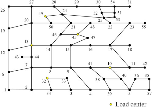
Figure 1. Urban road topology.

Table 1

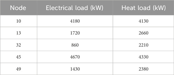
Table 1. Maximum electrical and heat loads during the planning period.

Figure 2

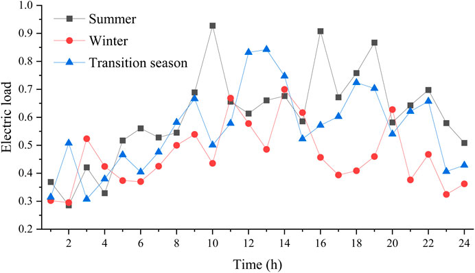
Figure 2. The curve of electrical load for typical operating scenarios.

Figure 3

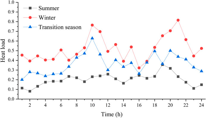
Figure 3. The curve of heat load for typical operating scenarios.

Figure 4

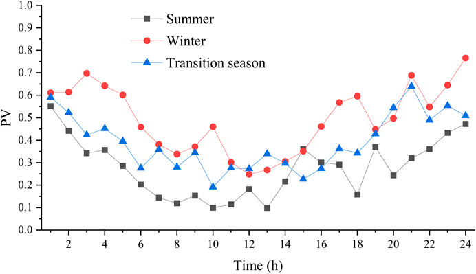
Figure 4. The curve of PV for typical operating scenarios.

Figure 5

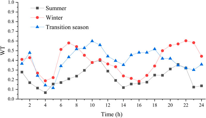
Figure 5. The curve of WT for typical operating scenarios.

Table 2

Table 2. Parameters of devices to be planned.

5.2 Analysis of the results of the proposed method

Figure 6 shows the results of energy station siting and energy supply network planning, Table 3 shows the results of device capacity allocation in the energy station, and Table 4 shows the various costs of the UIES.

Figure 6

Figure 6. Results of energy station siting and energy supply network planning.

Table 3

Table 3. Results of device capacity allocation in energy station.

Table 4

Table 4. Various costs of UIES.

As can be seen in Figure 1, the proposed method chooses to construct energy station at node 14 and constructs 15 power supply lines/heat pipes. The planned energy supply network does not have a ring network and satisfies the requirement of radial constraint. In order to further verify the effectiveness of the proposed method, the planning scheme and the total system cost are solved one by one when the energy station is constructed at other nodes, and the result reveals that the total cost of the planning scheme of the proposed method is one of the smallest. In summary, the proposed method can effectively plan the energy supply network.

As can be seen from Tables 3, 4, the proposed method in configures larger capacity PV and WT, which in conjunction with CHP can basically satisfy the electric load demand during the planning period, so the cost of purchasing electric in UIES is smaller. In addition, the proposed method configures a larger capacity of GB and a smaller capacity of EH, which means that the heat load is mainly satisfied by GB consuming gas, and is assisted by EH when more electric is generated in the region. This shows that the proposed method can reasonably plan the capacity of energy devices including CHP, GB, EH, PV, WT, and ES.

5.3 Analysis of the efficiency of the proposed heat network operation model

In order to analyze the efficiency of the proposed heat network operation model, the following scenario is set up as a comparison with the proposed method.

Case 1–1: Replace of the heat network operation model of the proposed method with the energy flow-based heat network operation model from Xue et al. (2021).

Table 6 demonstrates the comparison of UIES’s costs of the proposed method and Case 1–1. The results of energy station siting and energy supply network planning of Case 1–1 are the same as Figure 6. Figures 7, 8 show the total heat power of the heat equipment in the system of the proposed method and Case 1–1.

Figure 7

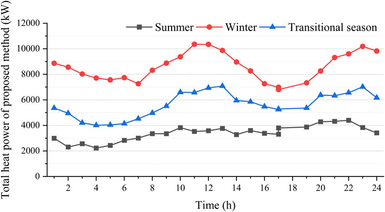
Figure 7. Total heat power of the heat equipment in the system of the proposed method.

Figure 8

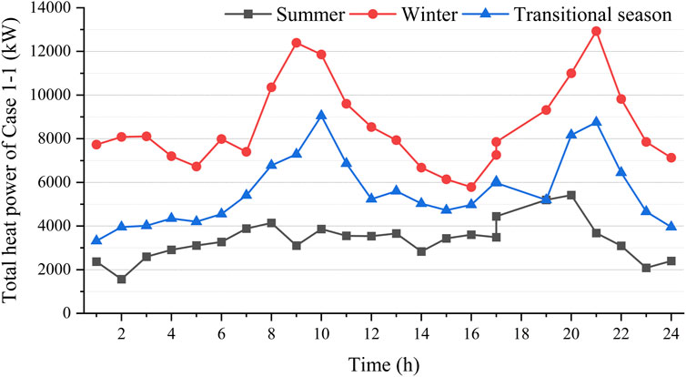
Figure 8. Total heat power of the heat equipment in the system of Case 1–1.

The comparison in Table 5 shows that compared to Case 1–1, the planning cost of proposed method is reduced by 5.79% and the operating cost is reduced by 3.98%, which in turn lead to a 5.15% reduction in the total cost. As can be seen from the comparison of Figures 7, 8, this is because considering the transmission delay can utilize the virtual heat storage characteristics of the heat network, which in turn smooths out the fluctuations of the heat power of the system and reduces the maximum power of heat load, thus reducing the required capacity of the heat equipment and lowering the investment cost and operation cost.

Table 5

Table 5. Comparison of UIES’s costs of the proposed method and Case 1–1.

5.4 Analysis of the impact of considering different devices on planning results

In order to analyze the impact of considering different devices on planning results, the following scenarios are set up as a comparison with the proposed method. Table 6 shows the comparison of the planning results.

Table 6

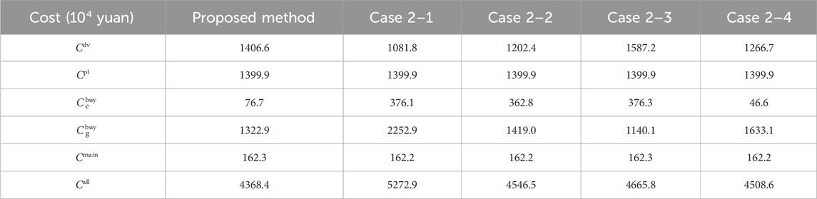
Table 6. Comparison of system costs in five scenarios.

Case 2–1: Planning for PV and WT is not considered.

Case 2–2: Planning for ES is not considered.

Case 2–3: Planning for GB is not considered.

Case 2–4: Planning for EH is not considered.

The comparison between the proposed method and Case 2–1 shows that in Case 2–1, the device investment cost for UIES is reduced because the planning for PV and WT is not considered, but UIES not only needs to purchase more electric from the superior grid, but also needs to purchase more natural gas for CHP generation, so the cost of purchasing electric and gas is significantly increased. Thus, in Case 2–1, although the investment cost for UIES is reduced by 11.6%, the total cost is increased by 20.7%.

The comparison between the proposed method and Case 2–2 shows that in Case 2–2, the device investment cost for UIES is reduced because the planning for ES is not considered, but the purchasing electric cost for UIES is significantly increased due to the absence of ES to provide peak shaving and valley filling. Thus, in Case 2–2, although the investment cost for UIES is reduced by 7.3%, the total cost is increased by 4.1%.

The comparison between the proposed method and Case 2–3 shows that in Case 2–3, not considering the planning for GB makes the purchasing gas cost for UIES decrease significantly, but the capacity of CHP and EH is increased in order to meet the heat load demand, which leads to an increase of the device investment cost and purchasing electric cost for UIES on the contrary, and consequently the total cost of the system increases by 6.8%.

The comparison between the proposed method and Case 2–4 shows that in Case 2–4, the purchasing electric cost for UIES is reduced due to the fact that EH is not considered in the planning, but the capacity of CHP and GB is increased in order to meet the heat load demand, which leads to an increase in the purchasing gas cost for UIES instead, and consequently the total cost of the system is increased by 3.2%.

In summary, it can be seen that the consideration of PV, WT, ES, EH, GB in station-network cooperative planning of UIES are all conducive to reducing the total cost of the system and improving the economics of the planning scheme.

6 Conclusion

In this paper, a station-network cooperative planning method of UIES based on energy flow model is proposed to realize the cooperative optimization of the siting and sizing of energy station and the topology of energy supply network. And the following conclusions are obtained through arithmetic example analysis: 1) The proposed method can effectively plan the energy supply network and reasonably configure the capacity of energy devices including CHP, GB, EH, PV, WT and ES.

2) Compared with the existing energy flow-based heat network operation model, the proposed method takes into account the transmission delay of the heat network, which can more fully utilize the heat storage capacity and thus improve the economic efficiency of the planning scheme.

3) The consideration of PV, WT, ES, EH, GB in station-network cooperative planning of UIES are all conducive to reducing the total cost of the system and improving the economics of the planning scheme.

Data availability statement

The original contributions presented in the study are included in the article/Supplementary Material, further inquiries can be directed to the corresponding author.

Author contributions

XF: Conceptualization, Methodology, Project administration, Resources, Software, Writing–original draft. SY: Conceptualization, Methodology, Software, Validation, Writing–original draft, Writing–review and editing. QH: Funding acquisition, Methodology, Software, Writing–original draft. LW: Data curation, Funding acquisition, Investigation, Visualization, Writing–original draft. CN: Investigation, Visualization, Writing–original draft. LY: Conceptualization, Project administration, Resources, Supervision, Validation, Writing–review and editing.

Funding

The author(s) declare that financial support was received for the research, authorship, and/or publication of this article. This work was funded by the Science and Technology Project of State Grid Jiangsu Electric Power Co., Ltd. (No. J2023083). The funder was not involved in the study design, collection, analysis, interpretation of data, the writing of this article, or the decision to submit it for publication.

Conflict of interest

Authors XF, QH, and LW were employed by the State Grid Wuxi Power Supply Company of Jiangsu Electric Power Co., Ltd.

The remaining authors declare that the research was conducted in the absence of any commercial or financial relationships that could be construed as a potential conflict of interest.

Publisher’s note

All claims expressed in this article are solely those of the authors and do not necessarily represent those of their affiliated organizations, or those of the publisher, the editors and the reviewers. Any product that may be evaluated in this article, or claim that may be made by its manufacturer, is not guaranteed or endorsed by the publisher.

Supplementary material

The Supplementary Material for this article can be found online at: https://www.frontiersin.org/articles/10.3389/fenrg.2024.1363822/full#supplementary-material

References

Baran, M., and Wu, F. (1989). Network reconfiguration in distribution systems for loss reduction and load balancing. IEEE Trans. Power Deliv. 4 (2), 1401–1407. doi:10.1109/61.25627

CrossRef Full Text | Google Scholar

Chen, C., Li, Y., Qiu, W., Liu, C., Zhang, Q., Li, Z., et al. (2022). Cooperative-game-based Day-Ahead scheduling of local integrated energy systems with Shared energy storage. IEEE Trans. Sustain. Energy 13 (4), 1994–2011. doi:10.1109/TSTE.2022.3176613

CrossRef Full Text | Google Scholar

Chen, C., Zhang, T., Wang, Y., Sun, G., Wu, C., and Lin, Z. (2024). Coordinated siting and sizing for integrated energy system considering generalized energy storage. Int. J. Electr. Power & Energy Syst. 155, 109619. doi:10.1016/j.ijepes.2023.109619

CrossRef Full Text | Google Scholar

Chen, C., Zhu, Y., Zhang, T., Li, Q., Li, Z., Liang, H., et al. (2023a). Two-stage multiple cooperative Games-based Joint planning for Shared energy storage provider and local integrated energy systems. Energy 284, 129114. doi:10.1016/j.energy.2023.129114

CrossRef Full Text | Google Scholar

Chen, S., Su, W., and Wu, B. (2023b). Two stage robust planning of park integrated energy system considering low carbon. Front. Energy Res. 10, 1100089. doi:10.3389/fevo.2022.1100089

CrossRef Full Text | Google Scholar

Chen, X., Wu, W., and Zhang, B. (2016). Robust Restoration method for active distribution networks. IEEE Trans. Power Syst. 31 (5), 4005–4015. doi:10.1109/TPWRS.2015.2503426

CrossRef Full Text | Google Scholar

Chen, Y., Lao, W., Qi, D., Hui, H., Yang, S., Yan, Y., et al. (2023c). Distributed Self-triggered Control for Frequency Restoration and active power Sharing in Islanded Microgrids. IEEE Trans. Industrial Inf. 19 (10), 10635–10646. doi:10.1109/TII.2023.3240738

CrossRef Full Text | Google Scholar

Dong, W., Lu, Z., He, L., Zhang, J., Ma, T., and Cao, X. (2023). Optimal expansion planning model for integrated energy system considering integrated demand Response and Bidirectional energy Exchange. CSEE J. Power Energy Syst. 9 (4), 1449–1459. doi:10.17775/CSEEJPES.2021.09220

CrossRef Full Text | Google Scholar

Dorfner, J., and Hamacher, T. (2014). Large-scale District heating network optimization. IEEE Trans. Smart Grid 5 (4), 1884–1891. doi:10.1109/TSG.2013.2295856

CrossRef Full Text | Google Scholar

Du, Y., Xue, Y., Wu, W., Shahidehpour, M., Shen, X., Wang, B., et al. (2024). Coordinated planning of integrated electric and heating system considering the optimal reconfiguration of District heating network. IEEE Trans. Power Syst. 39 (1), 794–808. doi:10.1109/TPWRS.2023.3242652

CrossRef Full Text | Google Scholar

Farrokhifar, M., Nie, Y., and Pozo, D. (2020). Energy systems planning: a Survey on models for integrated power and natural gas networks coordination. Appl. Energy 262, 114567. doi:10.1016/j.apenergy.2020.114567

CrossRef Full Text | Google Scholar

Ha, T., Xue, Y., Lin, K., Zhang, Y., Thang, V. V., and Nguyen, T. (2022). Optimal operation of energy hub based Micro-energy network with integration of renewables and energy storages. J. Mod. Power Syst. Clean Energy 10 (1), 100–108. doi:10.35833/MPCE.2020.000186

CrossRef Full Text | Google Scholar

Hong, B., Chen, J., Zhang, W., Shi, Z., Li, J., and Miao, W. (2018). Integrated energy system planning at Modular Regional-User level based on A two-layer bus structure. CSEE J. Power Energy Syst. 4 (No.2), 188–196. doi:10.17775/CSEEJPES.2018.00110

CrossRef Full Text | Google Scholar

Li, C., Li, P., Yu, H., Li, H., Zhao, J., Li, S., et al. (2021). Optimal planning of Community integrated energy station considering Frequency regulation Service. J. Mod. Power Syst. Clean Energy 9 (2), 264–273. doi:10.35833/MPCE.2019.000056

CrossRef Full Text | Google Scholar

Li, T., Han, X., Wu, W., and Sun, H. (2023). Robust expansion planning and Hardening strategy of meshed multi-energy distribution networks for resilience Enhancement. Appl. Energy 341, 121066. doi:10.1016/j.apenergy.2023.121066

CrossRef Full Text | Google Scholar

Liu, X. (2020a). Energy stations and pipe network collaborative planning of integrated energy system based on load complementary characteristics. Sustain. Energy Grids Netw. 23, 100374. doi:10.1016/j.segan.2020.100374

CrossRef Full Text | Google Scholar

Liu, X. (2020b). Pipeline network layout design of integrated energy system based on energy station site selection and load complementary characteristics. IEEE Access 8, 1–92790. doi:10.1109/ACCESS.2020.2991239

CrossRef Full Text | Google Scholar

Mu, Y., Chen, W., Yu, X., Jia, H., Hou, K., Wang, C., et al. (2020). A double-layer planning method for integrated community energy systems with varying energy conversion efficiencies. Appl. Energy 279, 115700. doi:10.1016/j.apenergy.2020.115700

CrossRef Full Text | Google Scholar

Strezoski, L., Padullaparti, H., Ding, F., and Baggu, M. (2022). Integration of utility distributed energy resource management system and aggregators for evolving distribution system operators. J. Mod. Power Syst. Clean Energy 10 (2), 277–285. doi:10.35833/MPCE.2021.000667

CrossRef Full Text | Google Scholar

Su, Y., Liu, F., Kang, K., and Wang, Z. (2023). Implicit sparsity of LinDistFlow model. IEEE Trans. Power Syst. 38 (5), 4966–4969. doi:10.1109/TPWRS.2023.3291214

CrossRef Full Text | Google Scholar

Wang, J., Du, W., and Yang, D. (2021). Integrated energy system planning based on life cycle and emergy theory. Front. Energy Res. 9, 713245. doi:10.3389/fenrg.2021.713245

CrossRef Full Text | Google Scholar

Wang, Y., Li, R., Dong, H., Ma, Y., Yang, J., Zhang, F., et al. (2019). Capacity planning and optimization of business park-level integrated energy system based on investment constraints. Energy 189, 116345. doi:10.1016/j.energy.2019.116345

CrossRef Full Text | Google Scholar

Wu, C., Gu, W., Jiang, P., Li, Z., Cai, H., and Li, B. (2018). Combined economic dispatch considering the time-delay of district heating network and multi-regional indoor temperature control. IEEE Trans. Sustain. Energy 9 (1), 118–127. doi:10.1109/TSTE.2017.2718031

CrossRef Full Text | Google Scholar

Xiao, H., Pei, W., Dong, Z., and Kong, L. (2018). Bi-Level planning for integrated energy systems incorporating demand response and energy storage under uncertain environments using novel metamodel. CSEE J. Power Energy Syst. 4 (2), 155–167. doi:10.17775/CSEEJPES.2017.01260

CrossRef Full Text | Google Scholar

Xue, Y., Shahidehpour, M., Pan, Z., Wang, B., Zhou, Q., Guo, Q., et al. (2021). Reconfiguration of district heating network for operational flexibility enhancement in power system unit commitment. IEEE Trans. Sustain. Energy 12 (2), 1161–1173. doi:10.1109/TSTE.2020.3036887

CrossRef Full Text | Google Scholar

Zhang, X., Shahidehpour, M., Alabdulwahab, A., and Abusorrah, A. (2015). Optimal expansion planning of energy hub with multiple energy infrastructures. IEEE Trans. Smart Grid 6 (5), 2302–2311. doi:10.1109/TSG.2015.2390640

CrossRef Full Text | Google Scholar

Zhang, Y., Li, J., Ji, X., Ye, P., Yu, D., and Zhang, B. (2023). Optimal Dispatching of electric-heat-Hydrogen integrated energy system based on Stackelberg game. Energy Convers. Econ. 4, 267–275. doi:10.1049/enc2.12094

CrossRef Full Text | Google Scholar