Influence of usage and model inaccuracies on the performance of smart hot water heaters: lessons learned from a demand response field test

Domestic hot water heaters are considered to be easily integrated as flexible loads for demand response. While literature grows on reproducible simulation and lab tests, real-world implementation in field tests considering state estimation and demand prediction-based model predictive control approaches is rare. This work reports the findings of a field test with 16 autonomous smart domestic hot water heaters. The heaters were equipped with a retrofittable sensor/actuator setup and a real-time price-driven model predictive control unit, which covers state estimation, demand prediction, and optimization of switching times. With the introduction of generic performance indicators (specific costs and thermal efficiency), the results achieved in the field are compared by simulations to standard control modes (instantaneous heating, hysteresis, night-only switching). To evaluate how model predictive control performance depends on the user demand prediction and state estimation accuracy, simulations assuming perfect predictions and state estimations are conducted based on the data measured in the field. Results prove the feasible benefit of RTP-based model predictive control in the field compared to a hysteresis-based standard control regarding cost reduction and efficiency increase but show a strong dependency on the degree of utilization.

1 Introduction

Historically, research on model predictive control (MPC) of domestic hot water heaters (DHWHs) for demand response (DR) followed a typical path. In the early days, researchers focused on theoretical considerations and simulation, followed by proof of concept studies in lab environments. In the last years, the first attempts to apply DHWHs in the field have been published. Generally, residential field tests published cover infrastructural and strategical issues (Shariatzadeh et al., 2015), technical and methodical aspects (Barbato and Capone, 2014), and economic or social impacts and acceptance (Darby and McKenna, 2012; Parrish et al., 2020). Although DHWHs are assumed to be one of the most promising devices for DR in the residential sector (Shan et al., 2016), field tests and smart grid implementation do not focus on the DHWH itself. Instead, DHWHs are mostly just seen as a specific form of the more generic concept of a shiftable load. This becomes apparent by the review of Kohlhepp et al. (2019) on field tests for residential thermal energy storage and their flexibility for DR. In the following, we discuss those field tests available in the literature that allow for an analysis specifically addressing DHWHs.

Hammerstrom et al. (2007) investigated 50 retrofitted DHWHs as grid-friendly appliances in the Pacific Northwest GridWise™ Testbed Demonstration Project. They switched off the appliances whenever the frequency of the grid fell below 59.95 Hz from the nominal 60 Hz used in the US. In a second approach of this project, they operated DHWHs on a real-time price (RTP) market via an automated control module considering participants’ comfort settings (Hammerstrom et al., 2008). In the EcoGrid EU Project (Aleixo et al., 2013), several DHWHs were simulated to show the cost reduction potential. Chassin and Kiesling (2008) reported on smart appliances including water heaters which were enabled to automatically respond to price signals. Svalstedt and Löf (2017) reported on the Smart Grid Gotland market test. DHWHs and other electrical residential loads were remotely controlled according to preset user comfort settings and according to special customer retail prices. D’hulst et al. (2015) deployed 15 DHWH with a DR control system in the LINEAR project, whereas user comfort settings had to be met. Maximum and minimum water temperature settings served as comfort requirements. A derived state of charge model and an indirect demand estimation based on power measurements were used to create flexibility.

In most field tests published, only incentives are used as input parameters and the DHWH is often modeled as a black box. This leads to aggregated results as a basis for scenario analysis whereas it is not possible to trace back a certain behavior of the superordinated energy system to a single DHWH or a single user. On the one hand, the necessary simplifications of field tests and their missing reproducibility compared to simulations and lab experiments are a major disadvantage. On the other hand, field tests are absolutely necessary to exploit the finding of simulations and lab experiments. Field tests allow us to analyze the technically achievable potential of MPC of DHWHs for DR.

Generally, published work of simulations and lab experiments follow a similar structure, both are reproducible, thus, exhibiting similar advantages. Various input parameters and assumptions can be included: different DHWH models, the state or state estimation of the DHWH, the knowledge or prediction of the user behavior, and the choice of different incentives (Engelbrecht et al., 2021; Heidari et al., 2021; Maltais and Gosselin, 2022). Based on this, simulations or lab experiments can be performed multiple times leading to a variety of results. These results can be evaluated individually for different setups, e.g., depending on each storage or demand. Additionally, the aforementioned reproducibility enables sensitivity analyses. Aggregating the results may even enable scenario studies on the behavior of multiple DHWHs within the superordinated energy system.

For an overview of simulation studies and lab experiments available in the literature, we refer, e.g., to the work of Kepplinger (2018) and Engelbrecht et al. (2021). We shortly discuss some recent publications to highlight typical shortcomings of purely simulation-based studies. Peirelinck et al. (Peirelinck et al., 2020) investigated the effect of pre-training a reinforcement learning agent for DHWHs in a price-driven DR control scenario. Compared to hysteresis control and MPC, the study showed that for a successful MPC implementation, a higher system identification effort is necessary compared to reinforcement learning approaches. On the other hand, reinforcement learning suffers from the training time of the models. The authors conclude that experimental tests have to be conducted to certainly quantify the state estimation error. Heidari et al. (2021) trained and compared several supervised learning methods for hot water demand prediction. Based on data collected from six residential homes, they tested the performance of a one-hour predictive control of the DHWH in a simulation environment using a random forest prediction model. Although the demand prediction is taken into account, the error due to system estimation is neglected in this study. Maltais and Gosselin (Maltais and Gosselin, 2022) proposed an MPC for DHWHs using a machine learning model to forecast user demand. They investigated the effect of user prediction errors on the results achieved. As the MPC assumed perfect system state knowledge, the error due to state estimation was not considered.

Next to the summarized key findings, the literature also gives a variety of insufficiently studied issues. Kohlhepp et al. (2019) state that model predictive control (MPC) for DR of DHWH has not been analyzed in field tests so far, although the potential of such a combination is clearly there. Further investigations are necessary, especially in combination with uncertainties. Patyn et al. (2018) define state estimation as a key for future research. Furthermore, no project with a special focus on DHWHs as appliances exist. Especially a deeper look into distributed autonomous and use-dependent control strategies as well as the technical challenges for even retrofittable systems is lacking.

To summarize: despite the high relevance to the community, the following research questions have not been answered so far.

• What is the technical-feasible potential of DHWHs for DR in retrofit applications?

• What is the DR potential by MPC under real-world conditions compared to standard modes of operation?

• What is the impact of errors due to user prediction and state estimation on the cost reduction and thermal efficiency in a practical achievable solution?

To answer these research questions, we combine the methods developed and investigated in two of our prior publications (Kepplinger et al., 2015; 2019) to derive and present our approach of combining a long-term field test with a simulation study in Section 2. In Section 3, we provide an analysis of the results gathered in the field. Based on simulations, we compare with alternative standard modes of operation and analyze the impact of user demand prediction and state estimation errors. Finally, we set our results into a greater perspective in the conclusion in Section 4.

2 Materials and methods

2.1 General framework

The general framework of the study comprises a field test and simulation studies as shown in Figure 1. As starting point, we present the development of our real-world field test of an MPC-based demand response approach for domestic hot water heaters with respect to hardware (retrofittable controller with sensors and actuators) and software (data handling, system identification, state estimation, demand prediction, and optimization) in Section 2.2.

Figure 1

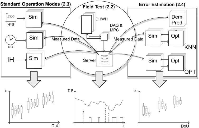
Figure 1. General framework of the study presented. The study reports on a field test, which tested an MPC approach for DR of DHWHs. Details on the field test are discussed in Section 2.2. Via simulations based on the data measured in the field, we mimic standard operation modes, namely, a hysteresis-based mode (HYS), a night-only heating mode (NO), and an instantaneous heating system (IH), these are described in detail in Section 2.3. To evaluate the impact of error due to state estimation and user prediction that has to be accounted for the real-world application of the field test, additional simulations are conducted assuming perfect knowledge of the system state (KNN) and the future demand (OPT). The methods used are described in Section 2.4. Based on the measurements and simulation results, we evaluate the degree of utilization (DoU - the fraction of daily energy use relative to the total exploitable heat capacity), specific costs, and thermal efficiency to analyze the technically feasible potential of the MPC approach in the field, the improvement compared to standard modes of operation, and the impact of prediction and estimation errors.

We integrate the data recorded in the field test into simulations. These simulations can be understood as idealized operation modes of the DHWH. They use a subset of the data measured in the field as disturbances (user demand, environment), system properties (heat transfer characteristics, capacity, set point temperatures), and the incentive (cost function). The simulation mimics the DHWH’s behavior, but differs in mode of operation, and, thus, leads to a differing output with respect to power consumption W_el(t) and DHWH system state. For all the simulations, a single-layer bulk model is used, where the system state is described by the average temperature only.

As a first category of comparative studies, simulations of the domestic hot water heaters under standard control strategies (instantaneous heating (IH), hysteresis control (HYS), and night tariff switching (NT)) are conducted (Section 2.3) to evaluate savings and performance.

As a second category, to quantify the influence of model and prediction errors on the savings achieved, the data collected is also used in simulations of the MPC approach (Section 2.4). First, considering perfect knowledge of the system state but predicting the demand (KNN) similarly to the routines implemented in the field. Second, considering perfect knowledge of the system state and the future demand (OPT). An overview of the different simulated operation modes and the assumptions associated is given in Table 1.

Table 1

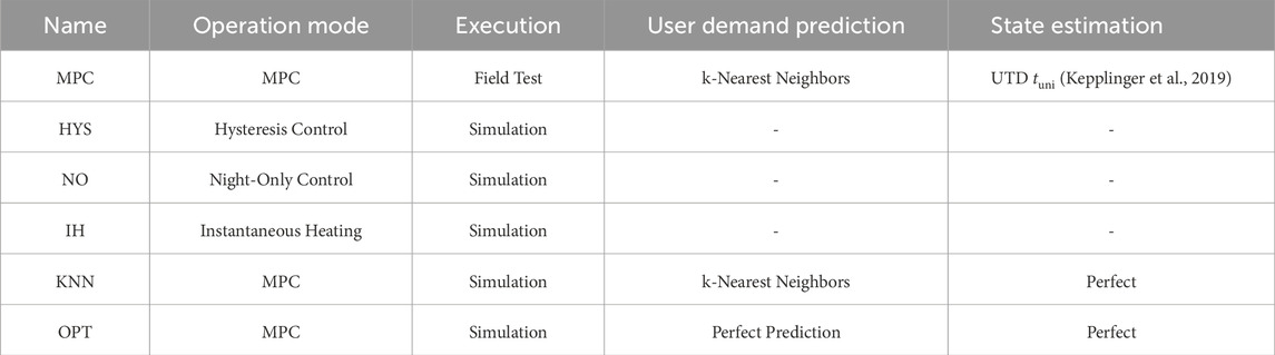
Table 1. Operation modes (real and simulated) considered for evaluation. In addition to the evaluation of the MPC mode during the field test, simulations of five different operation modes are conducted. These are based on the same user behavior and pricing regime but reflect either standard operation modes or idealized operation modes at different information statuses.

By introducing suitable key performance indicators (specific costs of electricity and thermal energy, thermal efficiency) we evaluate the performance of the field test (Section 3.1), compare it to standard operation modes (Section 3.2), and analyze errors (Section 3.3). Therefore, we introduce quantities and indicators for comparison. This approach combines real-world field test data with simulations and makes their results comparable.

2.2 Field test

In the Austrian Smart City Rheintal project (Eugster, 2016), we cooperated with the local energy supplier illwerke vkw and selected 16 homes with DHWHs to participate in the field test. These households of varying sizes rely on resistive hot water heaters for domestic hot water supply. The heaters were equipped with measuring, computing, and switching units. The DHWHs selected have a nominal volume of 120 l or 150 l and resistive heating elements located at the bottom of the tank with power ratings ranging from 1.9 kW to 2.5 kW. An overview of the metadata on the DHWHs considered in the study is given in Table 2. In the case of one flat, a change of tenants took place during the field test. This is why, a single heater (Heater ID 13) has been used by two different users (User IDs 13 and 14), and, thus, is listed separately. Prior to the field test, the DHWHs have been operated in the night-only (NO) operation mode. A signal (ripple control or time switch) activated the electrical power supply of the DHWH. For the cases investigated, this release time window referring to off-peak times was set from 10:30 p.m. to 06:00 a.m. by the distribution system operator.

Table 2

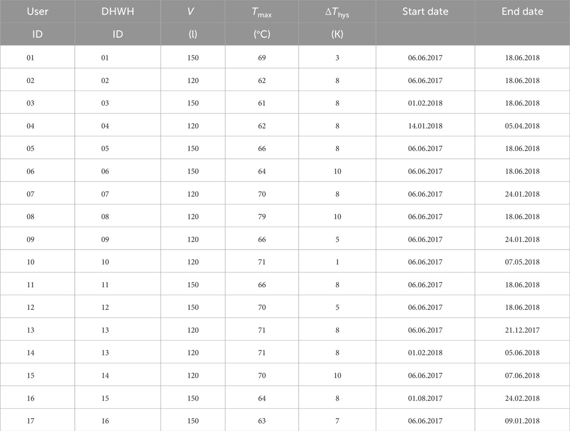
Table 2. User data evaluated in the field test. From left to right: User and heater ids; tank volume; set-point temperature; hysteresis temperature difference; start date of the evaluation; end date of the evaluation. Note that one DHWH (#13) has been used two times in the evaluation by different users (change of tenants) in the flat.

2.2.1 Hardware

Each of the 16 DHWHs was equipped with in-house-built hardware, as shown in Figure 2. This embedded system was designed to handle the data acquisition (DAQ) of the relevant physical values, receive a price signal via GSM, calculate the optimal switching times, and control the electricity supply of the DHWH accordingly. The choice of hardware was crucial as the goal was to develop a system that is easy to retrofit and would allow for a completely autonomous edge computing approach.

Figure 2

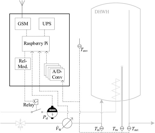
Figure 2. Setup and main components of the hardware developed for the field test. The hardware uses a Raspberry Pi for data acquisition (DAQ) and to run the MPC algorithm. The embedded system comprises a GSM module to receive electricity RTPs and store measurement data, an uninterruptible power supply, sensors partly including A/D converters to measure electric power consumption, water volume flow, as well as several temperatures (inlet, outlet, thermal well, and environment). Via a relay module the power supply of the DHWH can be interrupted.

A Raspberry Pi 2 Model B v1.1 was connected to various sensors. Water demand was measured using a volume flow meter with pulse output. The electric energy consumption was measured using a power meter. Four temperature sensors (thermocouples (TC), type K with A/D converters) were installed: one at both, the inlet (T_in) and outlet pipe (T_out) of the DHWH; at the immersion sleeve (thermal well) protruding inside the tank (T_tw); at the outside of the tank to measure the environment temperature (T_env). Table 3 shows relevant information (type, protocol, accuracy) on the measuring devices used.

Table 3

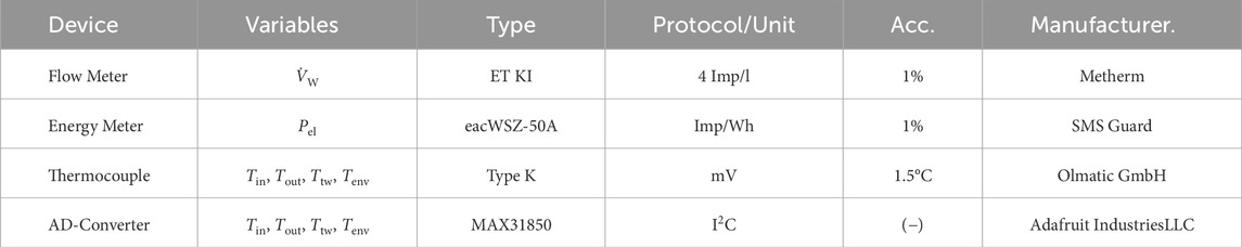
Table 3. Sensor devices used in the field test, including information on measured quantities and variables, types, manufacturer, protocol, accuracy, and references.

An uninterruptible power supply was installed to ensure reliability. In the event of a power failure, it continues to supply the RaspBerry Pi with power from a battery and, if necessary, shuts down the system in a controlled way.

The DHWH is switched via a commercially available relay (5V DC - 16A 250V AC) via the RasPiComm relay module from Amerscon.

The Fona telephone module from Adafruit with a corresponding M2M data tariff was used to communicate with a data server to receive the price signal and transmit the data collected for backup and monitoring of the devices.

2.2.2 Control routine

The software deployed on the embedded systems manages the individual tasks that are necessary for switching at optimal times. An overview of the main processes and data streams is provided in Figure 3. Following the approach of autonomous price-driven optimal control as published by the authors in (Kepplinger et al., 2015), an integer linear optimization problem minimizing the costs for heating is solved. The implementation is based on a bulk model of the heater constrained by a maximum and minimum average temperature limit. To apply such an approach, the model parameters (overall heat transfer coefficient UA and thermal capacitance C) and the current state of the system (average temperature in the tank T) have to be estimated, and hot water demand (Q_dem) to be predicted. For the latter, the k-nearest neighbor algorithm on the hot water demand data collected beforehand is used according to the method the authors proposed in (Kepplinger et al., 2015). For the former, the model parameters are identified based on historic data, and the system state is estimated periodically (please refer to our previous publication (Kepplinger et al., 2019) for more details). In the following, all processes of the software developed are discussed in detail.

Figure 3

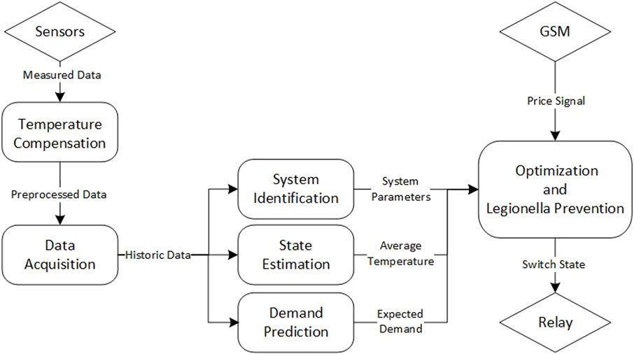
Figure 3. Main processes and data streams of the control routine. The measured data is preprocessed (temperature compensation) and stored locally (data acquisition). The historic data is used to identify optimal model parameters (system identification) of the DHWH. In turn, the model is used to estimate the current system state (state estimation) using the data from the measurements, providing an estimated average temperature inside the tank. Future hot water demand by the user is predicted based on historic data. Based on an MPC algorithm incentivized by the RTP signal (optimization) ensuring legionella prevention, the optimal switch state is derived and the relay is controlled.

2.2.3 Temperature compensation

Due to the unspecified accuracy of the temperature measurement, eight systems consisting of a thermocouple and an A/D converter were subjected to a temperature compensation procedure. For this purpose, these were exposed to different water temperatures in a heating bath and compared to reference temperature measurements with a sensor of known accuracy $\left(\pm 0.5\%\pm 0.5\text{K}\right)$ and a resolution of 0.1 K. A linear temperature compensation curve was derived from the determined values (analogous as in (Kepplinger et al., 2016)) showing a coefficient of determination of R² = 0.9993. The linear compensation function is given by T = p_slope ⋅ T_measured + T_offset with a slope of p_slope = 0.9759 and an offset of T_offset = 0.2299 °C. This compensation is applied during the process of data acquisition for all temperature measurements (T_tw, T_in, T_out, T_env).

2.2.4 Data acquisition

The data derived from the sensor measurements for the temperatures (T_in, T_out, T_tw, T_env), the hot water demand $({\dot{Q}}_{\text{dem}}={\dot{V}}_{\text{W}}{\rho }_{\text{W}}{c}_{\text{W}}(T_{\text{out}}-T_{\text{in}}))$ and the electric power (P_el) is stored directly on the SD card of the Raspberry Pi with a resolution of 1 minute. The constants c_W (J/kg/K) and ρ_W (kg/m³) refer to the water’s specific heat capacity and density, respectively. In the case of temperature sensors, the average of all measured values occurring in the current minute is saved. The sum of all occurring pulses per minute is counted and stored for the volumetric flow (water) meter and the electricity meter.

2.2.5 Model

For system identification, state estimation, and optimization, the change in energy stored within the heater has to be described. Therefore, we assume a uniform average temperature $\bar{T}$. Then, the transient energy balance for the DHWH being an open system reads

$C\frac{d\bar{T}}{dt}=-{\dot{Q}}_{\text{dem}}\left(t\right)+{\dot{W}}_{\text{el}}\left(t\right)-UA\left(\bar{T}\left(t\right)-T_{\infty }\right).(1)$

Here, ${\dot{Q}}_{\text{dem}}$ describes the power extracted due to hot water demand, ${\dot{W}}_{\text{el}}$ refers to the power supplied by the resistive heating element. The overall heat transfer coefficient UA describes the dynamics due to heat loss to the surroundings, and C refers to the thermal capacity of the DHWH. Assuming constant heating rate and energy demand for a given time interval $\left[t_0,t_0+\mathrm{\Delta }t\right]$, the analytic solution of Eq. 1 setting the initial condition $\bar{T}(t_0)={\bar{T}}_0$ is then given by

$\begin{array}{ll}\hfill \bar{T}\left(t_0+\mathrm{\Delta }t\right)& ={\bar{T}}_0{e}^{\left(-\frac{UA}{C}\mathrm{\Delta }t\right)}\hfill \\ \hfill & +\left(1-e^{\left(-\frac{UA}{C}\mathrm{\Delta }t\right)}\right)\left[\frac{{\dot{W}}_{\text{el}}}{UA}-\frac{{\dot{Q}}_{\text{dem,i}}}{UA}+T_{\infty }\right].\hfill \end{array}(2)$

2.2.6 System identification

We assume a uniform temperature distribution in the tank according to the model (cf. 2.2.5) to be reached as soon as the heating increased the thermal well temperature above the last hot water draw temperature at the outlet, i.e., T_tw (t_uni) > T_out (t_draw). This assumes stratification to be negligible, and, therefore, a single homogeneous temperature distribution inside the tank, i.e., $\tilde{T}(t)=T_{\text{tw}}(t)$. Here, $\tilde{T}(t)$ refers to the estimated average temperature in the tank. The uniform temperature distribution is assumed until the first hot water draw event after a heating cycle at t = t_cool, i.e., the end of a heating-up-cooling-off process. Defining ${\mathcal{T}}_{\text{UNI}}$ to be the set of all times assuming a uniform temperature distribution, i.e., the set consisting of several heating-up-cooling-off processes, the estimated system parameters $\widetilde{UA},\tilde{C}$ are derived via minimization of the RMSE as follows.

$\widetilde{UA},\tilde{C}=\arg \underset{UA,C}{\min }\sqrt{\frac{{\displaystyle \sum _{t\in {\mathcal{T}}_{\text{UNI}}}}{\left(\tilde{T}\left(t\right)-T_{\text{tw}}\left(t\right)\right)}^2}{|{\mathcal{T}}_{\text{UNI}}|}}.(3)$

Here, $\tilde{T}$ is calculated using Eq. 2. In our previous publication (Kepplinger et al., 2019), we were able to show that this model provides reasonable estimates for the average tank temperature at low computational costs. This model is referred to as the single node uniform temperature distribution model (1N UTD) with initialization at the end of the heating cycle (t_off).

2.2.7 State estimation

Using the system parameters resulting from Eq. 3, the state of the heater, i.e., the average tank temperature, is estimated by forward calculation of the model (Eq. 2) from the last end of a heating cycle, i.e., t_off. For optimization, this estimated average temperature serves as an input, cf. Figure 3. To solve the optimization procedure as described in Section 2.2.8, also the nominal power ${\bar{P}}_{\text{el}}$ has to be estimated. To this end, the maximum one-minute average value of the recorded electrical power is considered.

2.2.8 Optimization

We assume that the resistive heating element has a nominal power rating of ${\bar{P}}_{\text{el}}$ and the incentive is provided as vector $\mathbf{c}=\left(c_1,\dots ,c_N\right)$. Then, given the predicted hot water demand ${\dot{Q}}_{\text{dem}}$ by the user for the future time steps $i\in \left\{1,\dots ,N\right\}$, the optimization problem can be formulated as follows, by keeping the temperature at all times below T_max and above T_min in case of hot water demand.

$\begin{array}{ll}\hfill \underset{\mathbf{u}}{\min }& {\displaystyle \sum _{i=1}^N}{c}_i\cdot u_i\cdot {\bar{P}}_{\text{el}}\text{\hspace{0.17em}s.t.}\hfill \\ \hfill T_{\max }& \ge T_i\forall i\in \left\{1,\dots ,N\right\},\hfill \\ \hfill T_{\min }& \le T_i\forall i\in \left\{1,\dots ,N:{\dot{Q}}_{\text{dem},i}>0\right\}.\hfill \end{array}(4)$

By using the analytic solution of the bulk model as described in Eq. 2 of the heater, the constraints are linear (recursive solution), leading to a binary integer linear optimization problem, as derived already in (Kepplinger et al., 2015).

$\begin{array}{l}\hfill \underset{\mathbf{u}}{\min }{\displaystyle \sum _{i=1}^N}{c}_i\cdot u_i\cdot {\bar{P}}_{\text{el}}\text{\hspace{0.17em}s.t.}\\ \hfill A\mathbf{u}\le \mathbf{a},B\mathbf{u}\ge \mathbf{b},\end{array}(5)$

$\begin{array}{l}\hfill \lambda =e^{\left(-\frac{UA}{C}\mathrm{\Delta }t\right)}\\ \hfill A_{ij}=\left(1-\lambda \right){\lambda }^{i-1-j}\frac{{\bar{P}}_{\text{el}}}{UA},\\ \hfill a_i=T_{\max }-{\bar{T}}_0{\lambda }^i-{\displaystyle \sum _{j=0}^{i-1}}\left[\left(1-\lambda \right){\lambda }^{i-1-j}\left(T_{\infty }-\frac{{\dot{Q}}_{\text{dem,j}}}{UA}\right)\right],\\ \hfill B_{ij}=\left\{\begin{array}{cc}{A}_{ij},\hfill & \hfill {\dot{Q}}_{\text{dem},i}>0\\ 0,\hfill & \hfill {\dot{Q}}_{\text{dem},i}=0\end{array}\right.,\\ \hfill b_i=\left\{\begin{array}{cc}{T}_{\min }-T_{\max }+a_i,\hfill & {\dot{Q}}_{\text{dem},i}>0\hfill \\ 0,\hfill & {\dot{Q}}_{\text{dem},i}=0\hfill \end{array}\right..\end{array}(6)$

The hot water demand is predicted based on the recorded historic time series of demand via the DAQ. The future demand ${\dot{Q}}_{\text{dem}}(t)$ is determined using a Euclidean distance-based k-nearest neighbor algorithm (KNN) (Friedman et al., 1977). Here k refers to the number of best matches considered. To this end, the hot water demand of the past 12 hrs. is compared to the demand at the same time windows of historic days and the best k = 5 matches (daily demand profiles) are selected. The resulting prediction contains the matched historic data series for the optimization time window considered, which depends on the price signal available at the time of optimization, cf. 2.2.8. The optimization problem as stated in Eq. 4 thereby is subject to a maximum of 2N ⋅ k constraints (number of temperature constraints per timestep × number of time steps × number of nearest neighbors). If the optimization problem is infeasible due to the constraints imposed by the demand predicted, the number of nearest neighbors is reduced in steps of one, until a feasible solution is attained.

As Legionella pneumophila can thrive in hot water storages between 32°C and 42°C (Armstrong et al., 2014), an additional Legionella prevention is integrated into the optimization procedure. If, at the time of optimization, the measured thermal well temperature T_tw has not exceeded 55°C for the last 7 days, the heater is switched on until the set temperature is reached. As all heaters in the field test showed set point temperatures T_max above 60°C (cf. Table 2), sterilization time can even be expected to be below 10 min according to (Armstrong et al., 2014).

The spot market prices of the electricity exchange market in Austria are used as the price signal c of the optimization routine. These prices are published on a quarter-hour basis the day before at noon and are available online (EXAA Abwicklungsstelle für Energieprodukte AG, 2019). The existing data server automatically retrieves this data every day and distributes it to the individual DHWH control units via the GSM network. Every quarter hour the optimization routine is run to adapt to deviations of the user behavior from the prediction. Due to the fact that the next-day prices are available around noon and transmitted to the devices as soon as possible, the optimization time window varies between eight and 36 h. The optimization routine is run every quarter-hour solving the optimization problem given in Eq. 4, considering a discretization time step of Δt = 15 min.

2.3 Standard operation modes

To compare the results gathered in the field test to classic operation modes, we mimic the behavior of three standard modes of operation by simulation. The classic modes of operation of DHWHs exhibiting a storage volume are either time-of-use tariff-driven hysteresis, represented here by the night-only operation mode (NO), or a permanent hysteresis (HYS) control. Both controls reflect a hysteresis-based control that leads to an activation of the resistive heating element as soon as the measured temperature falls significantly below the temperature set point, defined by the hysteresis dead band. For both of these controls (NO, HYS), the same set point temperature T_set and dead band ΔT_hys are assumed as observed in the field test installations. For NO, an additional time window is set, which deactivates the resistive heating element completely outside of this time window. Within the time window, the heater works in hysteresis.

These two standard modes of operation (NO, HYS) are simulated using the bulk model solution (Eq. 1), using the same system characteristics as observed in the field (same capacities C, loss characteristics UA as well as set point temperatures T_set, hysteresis dead band ΔT_hys, and electric power rating of the resistive heating elements ${\bar{P}}_{\text{el}}$). The NO time window simulated is defined to match those applied in the area of the field test by the distribution system operator (from 10:30 p.m. to 06:00 a.m.), as to serve as a comparison mode to MPC. Measured data are used for hot water consumption ${\dot{Q}}_{\text{dem}}$ (defined by the water flow $\dot{V}$, as well as the temperatures at inlet T_in and outlet T_out), and the environment temperature T_env. Thereby, we are able to compare the output with respect to power consumption W_el(t), resulting costs, and DHWH system state, but match the other influences to those in the field.

Another solution to deliver domestic hot water at a single conduit are instantaneous water heating (IH) systems. These represent an extreme case for comparison, as no storage is needed. Therefore, the flexibility for load shifting is zero, but the thermal efficiency can be assumed to be perfect. For the simulation of the IH system, we set the electricity consumption equal to the hot water demand for simulation, i.e., W_el(t) = Q_dem(t).

2.4 Error estimation

The operation mode in the field test represents a specific approach to implement an autonomous price optimal control of the DHWHs. As can be seen in Figure 3, several processes are executed, which influence the decision on the relay state in the field (system identification (cf. 2.2.6), state estimation (cf. 2.2.7), demand prediction (cf. 2.2.8). To distinguish and compare the magnitude of those influences, several simulations are conducted.

These simulations can be understood as idealized operation modes of the DHWH. They use a subset of the data measured in the field, namely, the hot water consumption (based on water volume flow $\dot{V}$, temperatures at inlet T_in and outlet T_out) and the temperature of the environment T_env. The simulation mimics the DHWH’s behavior by using the same capacities C, loss characteristics UA as well as the electric power rating of the resistive heating elements ${\bar{P}}_{\text{el}}$. But the simulations differ in mode of operation, and, thus, lead to a differing output with respect to power consumption W_el(t), DHWH system state, and costs. For all the simulations, a single-layer bulk model is used, where the system state is described by the average temperature $\bar{T}$ only.

Each quarter-hour, the user prediction and optimization routines are executed as in the field test, but instead of using state estimation, the average temperature of the simulation is used as the current system state, representing perfect system knowledge. Two simulation studies are conducted to investigate the effect of errors due to state estimation and user prediction: 1) Optimal autonomous control (OPT) assumes perfect knowledge of the system state at all times as well as the future hot water demand. This is achieved by feeding the “future” hot water demand as a prediction to the optimization routine. 2) KNN-based autonomous control (KNN) only assumes perfect knowledge of the system states but includes the prediction of the user based on a KNN approach exactly as implemented in the field test, cf. 2.2.8. By comparison of the simulation results to those results achieved in the field, the performance of the methods used is evaluated. Moreover, the simulations allow us to relate and compare the results using real-world demand data to those found in simulation studies from the literature.

2.5 Evaluation

The evaluation of the data gathered in the field test aims to allow for 1) a comparison with existing results from the literature; 2) the quantification of the benefits of the method proposed with respect to energy efficiency and load shifting; and 3) an analysis of the effects due to state estimation and demand prediction. In the following, the data handling and preparation process is explained first.

Table 2 gives an overview of the participants evaluated in the field test. Not all evaluations show the same time window; first of all, due to varying duration in the installation of the in-house build hardware at the sites; Secondly, data showing acquisition gaps due to software or hardware issues were excluded. Taking these two aspects into account, the maximum possible time window of continuous operation has been selected for each participant to allow for a fair comparison and full analysis.

The data collected in the field test comprise results gathered in very heterogeneous settings, such as: A) the makeup of the households results in different hot water demands (usage times and amounts); B) the available hot water capacities are different depending on the type of the heater (120–150 l); and C) the data collected differs with respect to the evaluation period (duration and start/end date). To establish an evaluation that allows for comparison among this set of data and also with results from existing literature, quantities and indicators are used that are.

A) analyzable on arbitrary periods of time (e.g., days or months);

B) transferable between different setups (e.g., heaters of different volumes); and

C) applicable to the results of the simulated modes of operation (HYS, NO, IH, OPT, KNN).

The quantities derived are introduced and their significance explained hereafter, assuming a specific time period $\left[t_1,t_2\right]$.

Thermal efficiency for a DHWH is defined by

${\eta }_{\text{th}}=\frac{{\int }_{t_1}^{t_2}{\dot{Q}}_{\text{dem}}\left(t\right)\mathrm{d}t}{{\int }_{t_1}^{t_2}{\dot{W}}_{\text{el}}\left(t\right)\mathrm{d}t},(7)$

which by definition fulfills 0 ≤ η_th ≤ 1. For the instantaneous heating (IH) operation mode, the thermal efficiency always equals one.

Specific costs per consumed electricity (electric energy demand) and hot water (thermal energy demand) can be calculated by.

$c_{\text{el}}=\frac{{\int }_{t_1}^{t_2}c\left(t\right){\dot{W}}_{\text{el}}\left(t\right)\mathrm{d}t}{{\int }_{t_1}^{t_2}{\dot{W}}_{\text{el}}\left(t\right)\mathrm{d}t}\text{\hspace{0.17em}and}(8)$

$c_{\text{th}}=\frac{{\int }_{t_1}^{t_2}c\left(t\right){\dot{W}}_{\text{el}}\left(t\right)\mathrm{d}t}{{\int }_{t_1}^{t_2}{\dot{Q}}_{\text{dem}}\left(t\right)\mathrm{d}t}\text{,\hspace{0.17em}respectively.}(9)$

These quantities, both in (EUR/MWh), allow us to evaluate the performance of operation modes regarding their suitability to the real-time pricing regime. The simulated optimal operation (OPT) will provide the best result possible with respect to these specific costs, as it minimizes the real-time costs (nominator of Eq. 8) while assuming perfect demand prediction and system knowledge.

An important indicator to relate the domestic hot water usage (user dependent) and the system properties (capacity and set-point temperature) can be defined as the degree of utilization:

$q=\frac{{\int }_{t_1}^{t_2}{\dot{Q}}_{\text{dem}}\left(t\right)\mathrm{d}t}{\frac{\left(t_2-t_1\right)}{t_{\text{day}}}C}\text{,\hspace{0.17em}where}(10)$

$C=V{c}_{\text{W}}{\rho }_{\text{W}}\left(T_{\max }-T_{\min }\right)(11)$

defines the total exploitable heat capacity. The constants c_W (J/kg/K) and ρ_W (kg/m³) refer to the water’s specific heat capacity and density, respectively. The degree of utilization is based on a daily evaluation, thus, the total time considered is divided by the number of seconds per day t_day (s).

Additionally, we will examine the maximum heating cycle capacity, i.e., the maximum heat that ideally could be stored by fully heating the DHWH once from average inlet temperature ${\bar{T}}_{\text{in}}$ to T_max:

$C_{\max }=V{c}_{\text{W}}{\rho }_{\text{W}}\left(T_{\max }-{\bar{T}}_{\text{in}}\right).(12)$

In accordance, the total exploitable heat capacity C will also be referred to as the minimum heating cycle capacity.

3 Results and discussion

3.1 Field test results

First, we analyze the data collected in the field test for the different 17 users, equipped with the control unit. Figure 4 shows a 3-day period of measurements as collected in the field for user 4. It serves as an example to illustrate the data collected in the field test and explain the typical behavior of the MPC implemented. All measured quantities are depicted, including measured temperatures as well as the power and the RTP signal, which serves as an incentive for the optimization. It can be observed that the control based on quarter-hour RTP and demand prediction leads to short heating cycles as described in detail in our previous work (Kepplinger et al., 2019). Furthermore, it can be noticed that the heating cycles coincide with relatively low RTP values. The example data shows the effect of hot water being pushed back into the inlet pipe during heating cycles due to expansion, recorded by the inlet temperature sensor T_in positioned between the cold water inlet and the safety valve. This effect has also been discussed in detail based on lab experiments in our previous work (Kepplinger et al., 2019), as it might be a source of additional information to estimate the temperature distribution inside the storage tank. A large hot water draw-off event on the evening of August 21st can be observed, resulting in a thermal well temperature T_tw below the minimum set temperature T_min = 38°C. However, the outlet temperature T_out still shows values above the minimum set temperature.

To analyze the differences in usage, we compared the hot water demand to minimum (Eq. 11) and maximum heating cycle capacity (Eq. 12) in Figure 5 (left). User behavior has a substantial impact on the performance of the DR MPC approach. This is why strongly changing user behavior poses a significant challenge. To analyze the different users with respect to variance between single days, we calculated the classified days according to the degree of utilization q as defined in Eq. 10. Figure 5 (right) shows the relative share of days by the degree of utilization for all the users. From these two graphs, it can be seen that:

• 4 DHWHs are highly underused (3, 13, 14, 17),

• 3 DHWHs match the demand for the NO mode perfectly (2,12,16),

• 10 out of 17 (1, 4–11, 15) will not fulfill demand in NO mode.

This is due to the fact that NO mode assumes a single heating cycle during the night. These users would experience tap temperatures below the minimum temperature limit T_min in NO mode. This has to be taken into account, if the NO mode is compared to the MPC mode, as the optimization will adapt to higher demands by prediction and, thus, result in higher energy demand and costs.

Figure 4

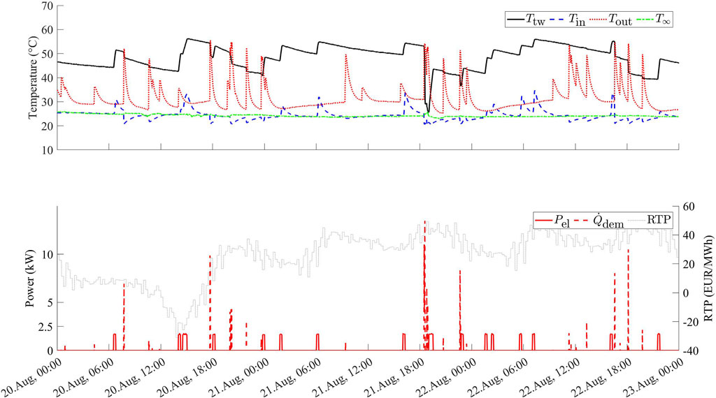
Figure 4. 3-day example showing the measured temperatures, power, and the RTP signal of User 4 in the field test.

Figure 5

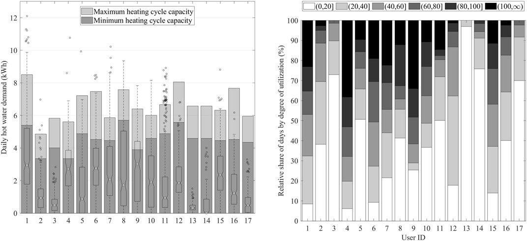
Figure 5. Usage of the different field test users. Left: Distribution of the daily hot water demand, compared to minimum and maximum heating cycle capacity of the single heater, C and C_max, respectively. The minimum and maximum heating cycle capacity reflect the energy that can be stored by fully heating the DHWH with reference to the minimum temperature limit or inlet temperature, respectively. These two quantities are dependent on heater volume, set point, and inlet temperature, as defined in Eqs 11, 12. Right: Relative share of days recorded classified by the degree of utilization q, as defined in Eq. 10.

3.2 Comparison to standard operation modes

To illustrate the behavior of the standard modes of operation (NO, HYS, IH) and compare it to the MPC implemented in the field test, Figure 6 shows the simulated tank temperatures and power for the same user and time window already considered before (Figure 4). The HYS mode results in demand-dependent heating of the storage as soon as the lower threshold value (set point temperature minus dead band) is reached. In the case of the NO mode, this hysteresis is only applied during night-time. It is clearly visible that the MPC results in shorter heating cycles strongly depending on the RTP value being the incentive for the optimization.

Figure 6

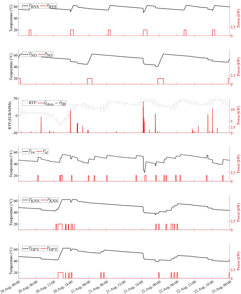
Figure 6. 3-day example (identical time window and user as in 4) showing the simulated (OPT, KNN, HYS, NO) and measured power and storage temperatures. Please note that the thermal well temperature and electrical power are measured quantities reflecting the MPC field test mode. The hot water demand (which equals the power for instantaneous heating) and the RTP are shown in one plot.

Figure 7 shows the change in specific costs for electricity and hot water consumption compared to the field test, if standard control strategies are considered (NO, HYS, IH). The results differ significantly for the different users. In most cases (14 of 17), instantaneous heating shows the highest specific costs for electricity, followed by standard hysteresis control. Thus, in all cases, the implemented MPC approach reduced electricity costs compared to the standard hysteresis control. Compared to NO control, MPC shows higher or lower specific electricity costs. This can be contributed to two factors mainly: First, the MPC control will always fulfill predicted hot water demands, thereby adapting to the user behavior, which might lead to higher energy consumption than in the case of the NO control. Second, the NO mode leads to heating cycles within the predefined time window at night, which at the RTP market considered are generally low.

Figure 7

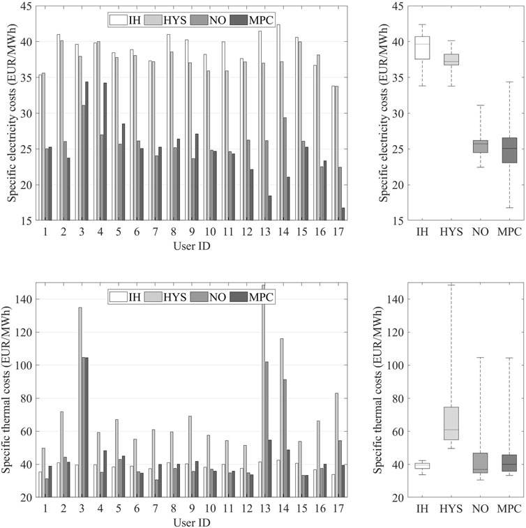
Figure 7. Specific electricity costs c_el (top) and specific thermal costs c_th (bottom) of standard control strategies (simulated) compared to the MPC field test results (measured). Left: Shown separately for all the different test field users. Right: Distribution of specific electricity costs for the different control strategies.

To take the different usage patterns into account, we analyzed the results for the standard control modes (IH, HYS, NO) and the field test (MPC) dependent on the degree of utilization. Results are shown in Figure 8. We classified all monthly data points, (t₂ − t₁ ≜ 1 month) of all DHWHs into 5 equidistant usage bins. If days or weeks are analyzed, the amount of energy stored in the DHWHs at the beginning or end of the period is significant compared to demand. To avoid these effects, we considered single months of DHWHs as one data point. By this, the averaging effect leads to results of higher quality but still creates a bigger set of data to be evaluated depending on the degree of utilization. For low degrees of utilization, the tested MPC approach achieves lower specific costs and higher thermal efficiencies compared to all standard control methods. As the use increases, NO mode on average becomes cheaper and more efficient compared to the MPC approach. Nevertheless, as explained before, NO mode may lead to cold tap events. The field test outperforms the classic HYS control mode, although the benefit regarding the specific electricity costs and thermal efficiency decreases with an increasing degree of utilization.

Figure 8

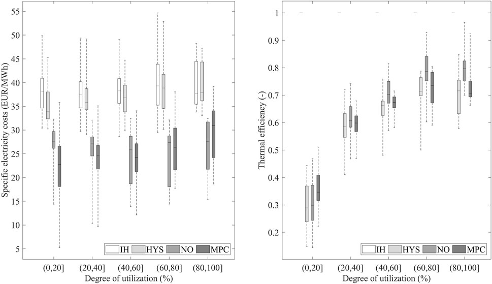
Figure 8. Specific electricity costs c_el (left) and thermal efficiency η_th (right) categorized by degree of utilization q for standard control modes (IH, HYS, NO) and the MPC field test. Every data point reflects a single consecutive month of user data.

3.3 Model and prediction error analysis

To illustrate the behavior of the optimization-based modes of operation (MPC, KNN, OPT), Figure 6 shows the measured or simulated tank temperatures and power. It is clearly visible that MPC, KNN, and OPT differ in switching times, as these depend on the specific results of state estimation and user demand prediction.

The MPC control of the field test relies on a state estimation and a user prediction. To study the effects of model and prediction inaccuracies on the results achieved, we analyze the difference in cost and efficiency improvements reached by the field test and the optimal MPC control strategies (KNN, OPT) simulated. As a basis for comparison, we use the simulation results of the hysteresis operation mode (HYS), as this is the most common control in current real-world systems. Figure 9 shows the relative change in electricity costs and thermal efficiencies compared to the HYS standard control mode.

Figure 9

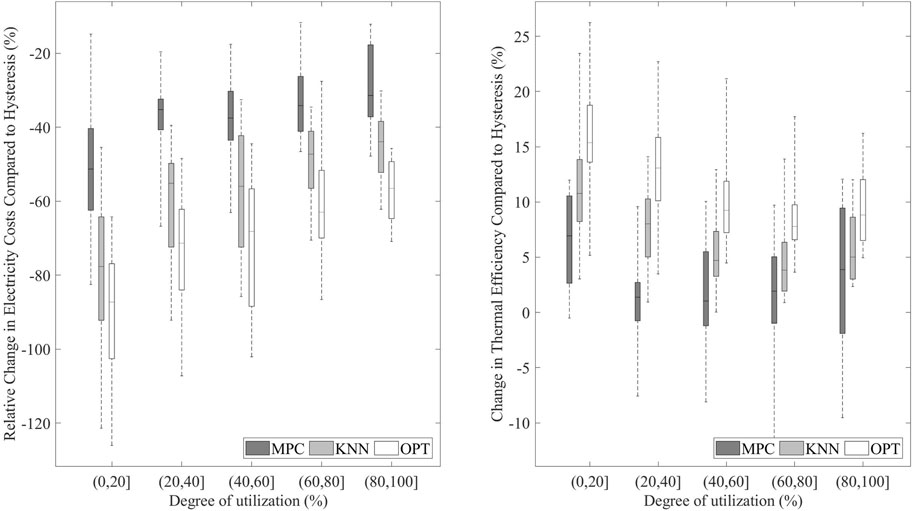
Figure 9. Relative change in the total electricity costs (left) and change in thermal efficiency η_th (right) reached by the optimization-based modes (MPC, KNN, OPT) compared to the hysteresis mode (HYS).

The cost achievable in a perfect and idealized setting are lowered significantly by assuming perfect prediction capabilities and state estimation. Or - to change the perspective: The technically feasible MPC solution in the field reaches significantly lower reductions in costs due to the errors contributed by demand prediction and state estimation. The optimal solution (OPT) leads to reductions of at least 50% for all degrees of utilization, and, due to negative RTPs, even can reach reductions of over 100% in case of extremely low user demand (0%–20% DoU). However, the control implemented in the field can only achieve around 40% reduction in average. For those periods of time and DHWHs where sizing matches user demand (60%–100%), sometimes even less than 20% are realized. Comparing the three optimization-based modes (MPC, KNN, OPT) shows that the error due to state estimation clearly has a larger impact than the error due to user prediction.

Increased thermal efficiency is a side-effect of optimization-based control, as the cost function of optimization reflects the product of price and electricity consumption. If the optimization procedure is based on perfect system knowledge and user prediction (OPT), an increase in thermal efficiency of at least 5% and up to about 25% for a low degree of utilization could be reached. In the field test, the thermal efficiency is slightly improved in average (1–7%), but in some cases is even lower than in standard operation mode.

3.4 Summary of results and discussion

To summarize the results observed in the field test and the simulation studies conducted, all performance indicators are provided in a single table (Table 4). The table also gives an overview of the sample size in the single degree of utilization classes.

Table 4

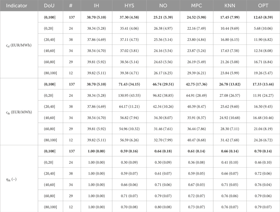
Table 4. Average (standard deviation) in specific electricity costs (c_el), specific thermal costs (c_th), and thermal efficiency specific electricity costs (η_th) for all modes of operation considered and separately listed for different degrees of utilization (DoU). # refers to the number of monthly data points in the bin.

Compared to NO operation mode, the results in the field test reduce the average specific electricity costs from 25.21 EUR/MWh (NO) by only 3%, whereas the optimal MPC modes reach average reductions of 30% (KNN) and 50% (OPT). According to our results, this is hard to be reached in real-world conditions with state-of-the-art methods, due to prediction and estimation errors.

Based on the average values, MPC lowers the average specific electricity costs by 34% from 37.3 EUR/MWh (HYS) to 24.52 EUR/MWh (MPC). In this case, the average specific electricity costs for the optimal MPC modes even decline to 17.45 EUR/MWh (53%) for KNN and to 12.63 EUR/MWh (66%) for OPT, respectively. The results also provide an explanation of the expected savings by MPC of DHWHs reported in the literature on simulation scenarios. Furthermore, it shows that the model inaccuracies and the prediction errors significantly reduce the technically achievable potential. The results suggest that the influence of the state estimation error is much more important than the error due to user prediction. As the latter is considered in many studies, but state estimation is mostly neglected, this result clearly suggests that further research needs to be focused on solutions for technically feasible state estimation concepts. As state estimation and the optimization model can not be considered independently from one another for a viable solution (cf. (Kepplinger et al., 2019)), further research should evaluate the suitability of different modeling approaches in the field.

4 Conclusion

To pave the way for scalable and sustainable MPC solutions for DHWHs, long-term field tests of prototypes under real-world environments are needed. We presented the results from a field test, where 16 DHWHs (comparably over 12 years of usage data) have been equipped with in-house developed hardware for an RTP-driven control, viable for a retrofitting solution. The software developed comprises routines for all processes necessary, from data acquisition, through state estimation and demand prediction, to optimization and operation.

To conclude on the realized load shift potential, and investigate estimation errors due to user prediction and model inaccuracies, we used the data gathered in the field test in simulation runs. We introduced indicators, which can be applied to different settings (prices, time periods, system parameters) and allow for comparison to simulated operation modes. Thereby we analyzed the dependence of specific electricity and thermal cost, as well as thermal efficiency on the degree of utilization.

The results show that the potential for load shifting is high enough to realize savings on the RTP market of 30% on average compared to hysteresis, which is the most common operation mode. However, the benefit of MPC with respect to costs and thermal efficiency declines as usage increases. This highlights the necessity in the field of DR to provide information on the degree of utilization underlying the studies presented.

Compared to the NO operation mode, which can be understood as a static DR approach being used in many Western countries for more than 30 years, the MPC-driven approach only showed economic benefits (specific electricity cost reduction based on RTP) for a low degree of utilization. However, it improved service quality through user prediction. Very importantly, it performs comparably but also allows for dynamically changing circumstances (e.g., strong fluctuation of renewable generation).

The investigation of the errors due to user prediction and state estimation showed that the error with respect to state estimation has a significantly higher impact on the cost reduction achieved than the error due to user prediction. As most literature on simulation studies considers user prediction but neglects state estimation, our results suggest that simulation studies so far overestimated the cost reduction and efficiency increase. This suggests that further research needs to be focused on solutions for technically feasible state estimation concepts. As state estimation and the optimization model can not be considered independently from one another for a viable solution, further research should evaluate the suitability of different modeling approaches in the field.

For the first time, we could verify the real potential of an MPC-based approach for DHWHs in the field and evaluate the impact of errors in demand prediction and state estimation. The approach proposed could serve the scientific community to gather more reliable and comparable results in both, reproducible simulation and lab environments, as well as in field test settings.

Future solutions proposed to integrate DHWHs for DR by MPC should focus on the evaluation of economic and energy conservation benefits in dependence on the degree of utilization. Errors from assumptions of perfect knowledge on disturbances (demand prediction) and system behavior (state estimation) need to be taken into account to allow for a fair comparison of the approaches discussed.

Data availability statement

The raw data supporting the conclusion of this article will be made available by the authors, without undue reservation.

Author contributions

PK: Conceptualization, Data curation, Formal Analysis, Investigation, Methodology, Software, Validation, Visualization, Writing–original draft, Writing–review and editing. GH: Conceptualization, Investigation, Methodology, Validation, Visualization, Writing–original draft. MP: Funding acquisition, Resources, Writing–review and editing.

Funding

The author(s) declare that financial support was received for the research, authorship, and/or publication of this article. We gratefully acknowledge financial support for the setup of the field test by the FFG–Austrian Research Promotion Agency within the frame-work of the SmartCity Rheintal project (FFG no. 836088). The financial support by the Austrian Federal Ministry for Digital and Economic Affairs and the National Foundation for Research, Technology and Development and the Christian Doppler Research Association is gratefully acknowledged.

Conflict of interest

The authors declare that the research was conducted in the absence of any commercial or financial relationships that could be construed as a potential conflict of interest.

Publisher’s note

All claims expressed in this article are solely those of the authors and do not necessarily represent those of their affiliated organizations, or those of the publisher, the editors and the reviewers. Any product that may be evaluated in this article, or claim that may be made by its manufacturer, is not guaranteed or endorsed by the publisher.

References

Aleixo, L., Morch, A. Z., Rosin, A., Grande, O. S., Saele, H., and Palu, I. (2013). “Ecogrid eu project-real time price based load control and economic benefits in a wind production based system,” in 22nd international conference and exhibition on electricity distribution (CIRED 2013). Stockholm: (IET), 1–4. doi:10.1049/cp.2013.1253

CrossRef Full Text | Google Scholar

Armstrong, P. M., Uapipatanakul, M., Thompson, I., Ager, D., and McCulloch, M. (2014). Thermal and sanitary performance of domestic hot water cylinders: conflicting requirements. Appl. energy 131, 171–179. doi:10.1016/j.apenergy.2014.06.021

CrossRef Full Text | Google Scholar

Barbato, A., and Capone, A. (2014). Optimization models and methods for demand-side management of residential users: a survey. Energies 7, 5787–5824. doi:10.3390/en7095787

CrossRef Full Text | Google Scholar

Chassin, D. P., and Kiesling, L. (2008). Decentralized coordination through digital technology, dynamic pricing, and customer-driven control: the gridwise testbed demonstration project. Electr. J. 21, 51–59. doi:10.1016/j.tej.2008.09.002

CrossRef Full Text | Google Scholar

Darby, S. J., and McKenna, E. (2012). Social implications of residential demand response in cool temperate climates. Energy Policy 49, 759–769. doi:10.1016/j.enpol.2012.07.026

CrossRef Full Text | Google Scholar

D’hulst, R., Labeeuw, W., Beusen, B., Claessens, S., Deconinck, G., and Vanthournout, K. (2015). Demand response flexibility and flexibility potential of residential smart appliances: experiences from large pilot test in Belgium. Appl. Energy 155, 79–90. doi:10.1016/j.apenergy.2015.05.101

CrossRef Full Text | Google Scholar

Engelbrecht, J., Ritchie, M. J., and Booysen, M. (2021). Optimal schedule and temperature control of stratified water heaters. Energy Sustain. Dev. 62, 67–81. doi:10.1016/j.esd.2021.03.009

CrossRef Full Text | Google Scholar

Eugster, C. (2016) “Smart city rheintal–elements for the emission and energy related spatial development of the polycentric structured rhine-valley,” in Klima und Energiefonds. Final report.

Google Scholar

EXAA Abwicklungsstelle für Energieprodukte AG (2019). Historical market data. Available at: https://www.exaa.at/marktdaten/historische-marktdaten/(Accessed December 17, 2019).

Google Scholar

Friedman, J. H., Bentley, J. L., Finkel, R. A., et al. (1977). An algorithm for finding best matches in logarithmic expected time. ACM Transactions on Mathematical Software (TOMS) 3 3, 209–226. doi:10.1109/tc.1977.1674849

CrossRef Full Text | Google Scholar

Hammerstrom, D. J., Ambrosio, R., Carlon, T. A., DeSteese, J. G., Horst, G. R., Kajfasz, R., et al. (2008) Pacific Northwest GridWise^TMtestbed demonstration projects; Part I. Olympic peninsula project. Tech. Rep. Richland, WA (United States): Pacific Northwest National Lab.

Google Scholar

Hammerstrom, D. J., Brous, J., Chassin, D. P., Horst, G. R., Kajfasz, R., Michie, P., et al. (2007) Pacific northwest gridwise^TMtestbed demonstration projects; part ii. grid friendly^TMappliance project. Tech. rep. Richland, WA (United States): Pacific Northwest National Lab.

Google Scholar

Heidari, A., Olsen, N., Mermod, P., Alahi, A., and Khovalyg, D. (2021). Adaptive hot water production based on supervised learning. Sustain. Cities Soc. 66, 102625. doi:10.1016/j.scs.2020.102625

CrossRef Full Text | Google Scholar

Kepplinger, P. (2018) Autonomous demand side management of domestic hot water heaters. Austria: University of Innsbruck. Ph.D. thesis.

Google Scholar

Kepplinger, P., Huber, G., and Petrasch, J. (2015). Autonomous optimal control for demand side management with resistive domestic hot water heaters using linear optimization. Energy Build. 100, 50–55. doi:10.1016/j.enbuild.2014.12.016

CrossRef Full Text | Google Scholar

Kepplinger, P., Huber, G., and Petrasch, J. (2016). Field testing of demand side management via autonomous optimal control of a domestic hot water heater. Energy Build. 127, 730–735. doi:10.1016/j.enbuild.2016.06.021

CrossRef Full Text | Google Scholar

Kepplinger, P., Huber, G., Preißinger, M., and Petrasch, J. (2019). State estimation of resistive domestic hot water heaters in arbitrary operation modes for demand side management. Therm. Sci. Eng. Prog. 9, 94–109. doi:10.1016/j.tsep.2018.11.003

CrossRef Full Text | Google Scholar

Kohlhepp, P., Harb, H., Wolisz, H., Waczowicz, S., Müller, D., and Hagenmeyer, V. (2019). Large-scale grid integration of residential thermal energy storages as demand-side flexibility resource: a review of international field studies. Renew. Sustain. Energy Rev. 101, 527–547. doi:10.1016/j.rser.2018.09.045

CrossRef Full Text | Google Scholar

Maltais, L.-G., and Gosselin, L. (2022). Energy management of domestic hot water systems with model predictive control and demand forecast based on machine learning. Energy Convers. Manag. X 15, 100254. doi:10.1016/j.ecmx.2022.100254

CrossRef Full Text | Google Scholar

Parrish, B., Heptonstall, P., Gross, R., and Sovacool, B. K. (2020). A systematic review of motivations, enablers and barriers for consumer engagement with residential demand response. Energy Policy 138, 111221. doi:10.1016/j.enpol.2019.111221

CrossRef Full Text | Google Scholar

Patyn, C., Peirelinck, T., Deconinck, G., and Nowe, A. (2018). “Intelligent electric water heater control with varying state information,” in 2018 IEEE international conference on communications, control, and computing technologies for smart grids (SmartGridComm) (IEEE), 1–6.

CrossRef Full Text | Google Scholar

Peirelinck, T., Hermans, C., Spiessens, F., and Deconinck, G. (2020). Domain randomization for demand response of an electric water heater. IEEE Trans. Smart Grid 12, 1370–1379. doi:10.1109/tsg.2020.3024656

CrossRef Full Text | Google Scholar

Shan, K., Wang, S., Yan, C., and Xiao, F. (2016). Building demand response and control methods for smart grids: a review. Sci. Technol. Built Environ. 22, 692–704. doi:10.1080/23744731.2016.1192878

CrossRef Full Text | Google Scholar

Shariatzadeh, F., Mandal, P., and Srivastava, A. K. (2015). Demand response for sustainable energy systems: a review, application and implementation strategy. Renew. Sustain. Energy Rev. 45, 343–350. doi:10.1016/j.rser.2015.01.062

CrossRef Full Text | Google Scholar

Svalstedt, C., and Löf, M. (2017). Behaviour of active household customers on the electricity market–findings from market test smart grid gotland. CIRED-Open Access Proc. J. 2017, 2624–2627. doi:10.1049/oap-cired.2017.0744

CrossRef Full Text | Google Scholar