Optimal demand response scheduling and voltage reinforcement in distribution grids incorporating uncertainties of energy resources, placement of energy storages, and aggregated flexible loads

Instead of expanding power plant capacities, which is an extremely expensive investment option, demand response offers an economical solution to the challenges arising from the variability and intermittency of the renewable energy resources and demand variations, particularly during demand peak periods. This paper proposes a multi-objective optimization framework for the optimal power flow problem that integrates a stepwise demand response involving flexible and aggregated loads. The process includes short-term demand forecasting using long short-term memory (LSTM) networks in a smart distribution grid, followed by the optimal allocation of energy storage systems, and load aggregators. By determining the optimal solution point of the multi-objective problem analytically, significant system costs and peak demand can be reduced without compromising system stability. Through numerical studies for a sample study case, a reduction of 22% in system costs, 2% in total voltage variation, and 10% in peak demand is observed for a negligible impact on customers’ convenience.

1 Introduction

Demand response (DR) is an important feature of smart grids and aims to change the consumption pattern of end-uses from their normal patterns to reduce the network’s peak demand and shift the loads to network’s off-peak periods (Albadi and El-Saadany, 2008). While DR has been widely employed in industrial and commercial sectors since 1970, it is being expanded thanks to technology developments and market improvements (Henríquez et al., 2017). Although consumers are technically capable of reducing their demand quickly and reliably, implementing DR for industrial loads can be more challenging than that for residential loads, primarily because industrial plants require more stringent reliability management (Shoreh et al., 2016). On the other hand, residential sector accounts for the a very large share of electricity consumption (e.g., 38% in the United States) (Buildings Energy Data Book, 2011). Heating, ventilation, and air conditioning (HVAC) systems constitute an important part of energy consumption in our daily lives; for example, approximately 40% of the energy consumption of buildings in the United States is related to HVAC systems (Bhattacharya et al., 2017). Aggregated domestic and commercial loads can be used in the DR program. To manage the flexibility of a large number of scattered DR resources in the context of electricity markets, they must be aggregated by a new participant called the DR aggregator (Henríquez et al., 2017). Aggregators can be used for any type of small-scale and high-potential flexible loads. As an example, HVAC aggregators (HVACA) enable owners to participate in DR by aggregating a number of HVAC units. In fact, without going out of the standard temperature range, it is possible to provide the desired temperature and reduce energy consumption simply by applying the predicted load chart in the process and settings, bringing a win-win situation for smart grid operators and consumers. In fact, with peak shaving via DR, the operator brings less expensive power plants into operation, therefore, reducing the cost of the entire system.

The core of a proficient power markets is the optimal power flow (OPF) challenge from economic, electrical, and computational standpoints. Economically, achieving an effective market equilibrium necessitates multi-faceted nonlinear pricing mechanisms. Electrically, the power flow is characterized by alternating current (AC), thereby introducing supplementary nonlinear elements. Computationally, the optimization process entails non-convexities, encompassing binary variables and continuous functions, rendering the problem arduous to resolve (Cain et al., 2012). The quadratic and non-linear characteristics of the power flow equations of the ac power grid make the OPF problem non-convex. Therefore, solutions such as the convex relaxation and linear approximation methods have been proposed to simplify the AC-OPF problem (Nakabi and Toivanen, 2021). The convex relaxations methods are generally shown to be exact only under certain conditions (Chowdhury et al., 2023). One of the linear approximation methods applied in the transmission network is DCOPF, but due to very small phase changes (Li et al., 2023), this method is not suitable for the distribution network. According to (Nair et al., 2022), among the three formulation methods of AC-OPF, the power balance polar formulation is the best choice for small distribution grids because of its fast runtime.

Integration of the AC-OPF problem with DR has been the focus of several studies. Emphasizing the importance of the AC-OPF problem, in some references, such as (Younesi et al., 2024), where the problem is solved in the electricity market framework, the AC-OPF structure is used to ensure the minimization of lost load and enhance resilience. In (Vanin et al., 2022) an mixed-integer linearized OPF-based congestion mitigation strategy is presented for DR in unbalanced residential networks. The strategy is based on requiring residential customers to limit their demand for a certain amount of time in exchange for economic benefits. A time-value-based demand-shifting strategy is proposed for DR in (Jabari et al., 2020) which is focused on transmission system and only active power. The article by (Khonji et al., 2016) has investigated OPF in the context of utility-maximizing DR management in distribution networks, in which customers’ demands are satisfied subject to the operating constraints of voltage and transmission power capacity. An optimal DR-based AC-OPF problem considering renewable energies and energy storage systems (ESSs) has been presented in (Zarei and Ghaffarzadeh, 2023) for a transmission network with short-term load forecasts using long short-term memory networks (LSTM). Considering the constant power factor for before and after DR, active and reactive power are included in the problem at the same time. In (Mak et al., 2023; Merrad et al., 2022), machine-learning approaches are used to solve AC-OPF problems in a decentralized fashion, but challenges related to its accuracy are still not solved, especially in systems with a high number of buses (such as the distribution network).

At present, the direct integration of AC-OPF with DR has been the subject of only a few studies. This study introduces a DR-based strategy for the AC-OPF problem, focusing on the aggregator’s small-scale flexible HVAC loads and the direct participation of flexible distributed loads at distribution grid buses, considering their simultaneous effects. The paper also discusses LSTM-based load prediction, the optimal placement of ESSs, and an intelligent model for HVACAs that prioritizes the user’s desired temperature range. Uncertainties in distributed energy resources (DERs) are modeled using a scenario-based approach and factored into optimal scheduling. The proposed scheme has the potential to significantly delay or eliminate the need to construct a new power plant by leveraging the participation of a small portion of the loads in the distribution network. The multi-objective model presented in the paper leads to a substantial reduction in total system costs, minimizes total voltage variations, and levels out the electrical load pattern while maintaining user convenience.

The key contributions of this paper to the research field can be summarized as below:

• Developing a simultaneous two-part DR strategy involving aggregated small-scale flexible HVAC loads and partial flexible loads across different load buses.

• Formulating a multi-objective optimization of the AC-OPF problem through an analytical approach that integrates DR considerations, aiming to reduce the total system costs, peak loads, and total voltage variations while enhancing user convenience.

• Optimizing the allocation of Energy Storage Systems (ESSs) within the smart distribution grid, utilizing a modified LSTM-based method for short-term load prediction, and implementing intelligent control for HVACA based on predicted load patterns to maintain the desired temperature ranges for residents.

The remainder of this paper is organized as follows: The proposal along with the formulated objective function are introduced in Section 2. Section 3 presents the performance evaluation of the proposal using numerical studies. Finally, the key findings of the research are summarized and presented in Section 4.

2 The proposal

First, the electrical demand was predicted based on previous consumption data using the LSTM method. Then, optimal locations for ESSs were selected in the structure of the smart distribution grid, which included distributed energy sources, such as small DGs, solar and wind units, and thermal units. In addition, multiple scenarios for wind and solar units have been developed to consider the uncertainty of renewable energy sources. An HVACA was integrated into the network based on its network structure and capacity. This aggregator was modeled by considering the min/max margin temperature and the predicted load patterns. Subsequently, a multi-objective problem was modeled and simulated within the AC-OPF framework, considering the relative response of all distribution network buses to DR programs, as well as two modes for the HVACA: flexible and non-flexible. Finally, an analytical method was used for optimal solution selection. The overall solution procedure is illustrated in Figure 1.

Figure 1

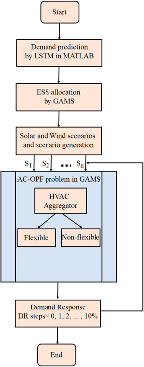
Figure 1. Flowchart of the proposal.

2.1 Objective functions

The proposed multi-objective function comprises one economic, two technical, and one user-convenience functions, as introduced and discussed below:

2.1.1 Total Cost Function

The total cost function incorporates the costs of active and reactive power generation, load shedding, and wind/solar curtailment, given by

$O{F}_1=a_g{P_{i,t}^g}^2+b_g{P}_{i,t}^g+c_g+c\cdot Q_{i,t}^g+{\displaystyle \sum _{i,t}}VOLL\times P_{i,t}^{LS}+{\displaystyle \sum _{i,t}}VOLW\times P_{i,t}^{WC}+{\displaystyle \sum _{i,t}}VOLS\times P_{i,t}^{SC}(1)$

and should be minimized. In (1), a_g, b_g, c_g, and c are the fuel cost coefficients of active and reactive power generation at unit g, respectively. P_i,t^g, P_i,t^LS, P_i,t^WC, and P_i,t^SC are the power generation of unit i, active load shedding in bus i, and wind and solar curtailment in bus i, at time t respectively. To simplify the problem, the quadratic cost function of thermal power plants was approximated as a first-order function. VOLL is the value of the load loss according to the graph of wind and demand changes, which is considered as a penalty (Gorman, 2022). Similarly, VOLW/VOLS is the cost factor for reducing wind/solar energy production in wind/solar power plants, according to the graph of wind/solar and demand changes.

2.1.2 Power quality improvement

In the pursuit of enhancing voltage stability, an objective function is formulated to reduce the voltage deviations across all nodes within the power grid, in the form of

$O{F}_2={\displaystyle \sum _{t=1}^T}{\displaystyle \sum _{i=1}^N}\left|V_{t,i}-V_{t,i}^{*}\right|(2)$

in which the voltage deviation function is used to enhance the voltage profile and power quality, where V_t,i is the voltage at bus i at time t, and V_t,i^* is set to one in this study.

2.1.3 Peak reduction

The equation for the peak reduction is presented in reference (Aalami et al., 2010). An objective function is introduced to incorporate the peak reduction of active power before and after DR, in the form of

$O{F}_3=\frac{P_{load}^{new}-P_{load}^{old}}{P_{load}^{old}}\times 100(3)$

which is highly important during the hot seasons of the year for effectively managing customers’ electricity consumption.

2.1.4 User convenience

To account for the diverse range of network loads, the similarity between the load profiles with and without DR is evaluated using the correlation coefficient, which is then incorporated as the fourth objective function in the final assessment, in the form of

$O{F}_4=\raisebox{1ex}{$\left({\displaystyle \sum _{t=1}^{24}}\left(P_{load}^{new}\left(t\right)-\overline{P_{load}^{new}}\right)\left(P_{load}^{old}\left(t\right)-\overline{P_{load}^{old}}\right)\right)$}\!\left/ \!\raisebox{-1ex}{$\left(\sqrt{{\displaystyle \sum _{t=1}^{24}}{\left(P_{load}^{new}\left(t\right)-\overline{P_{load}^{new}}\right)}^2\cdot {\displaystyle \sum _{t=1}^{24}}{\left(P_{load}^{old}\left(t\right)-\overline{P_{load}^{old}}\right)}^2}\right)$}\right.(4)$

$\overline{P_{load}^{new}}=\left({\displaystyle \sum _{t=1}^{24}}{P}_{load}^{new}\left(t\right)\right)/24(5)$

$\overline{P_{load}^{old}}=\left({\displaystyle \sum _{t=1}^{24}}{P}_{load}^{old}\left(t\right)\right)/24(6)$

2.2 Uncertainty of distributed energy resources

To consider the effect of distributed energy resources such as wind and solar units, all OF_j are calculated in every possible scenario (S_i) and then combined in the form of

$O{F}_j={\displaystyle \sum _{S_1}^{S_n}}\frac{P_{\left(S_i\right)}\cdot O{F}_j^{S_i}}{100}(7)$

where OF_j^S_i and P(s_i) are respectively the values of OF_j in scenario S_i and the probability of scenario S_i.

2.3 Technical constraints

The constraints for the operation of the thermal power plants, load-shedding limits, as well as operation of ESSs and distributed energy resources should be considered for the successful implementation of the DR, as introduced and discussed below:

2.3.1 Thermal power plant constraints

The constraints regarding the upper and lower limits of active and reactive power generation from thermal power plants, as well as their ramp-up and down rates, are given by

$P_{i,t}^{g,\min }\le P_{i,t}^g\le P_{i,t}^{g,\max }(8)$

$Q_{i,t}^{g,\min }\le Q_{i,t}^g\le Q_{i,t}^{g,\max }(9)$

$P_{i,t+1}^g-P_{i,t}^g\le R{U}_g(10)$

$P_{i,t-1}^g-P_{i,t}^g\le R{D}_g(11)$

2.3.2 Load shedding constraints

To determine the cost of load shedding, the curtailed demand of each bus should be within the range of zero to the nominal load capacity of that bus, given by

$0\le P_{i,t}^{LS}\le P_{i,t}^L(12)$

$0\le Q_{i,t}^{LS}\le Q_{i,t}^L(13)$

2.3.3 ESS constraints

The constraints pertaining to ESSs are given by (Thanh et al., 2022; Nan et al., 2017)

$SO{C}_t=SO{C}_{t-1}+\left(P_t^{ch}{\eta }_{ch}-P_t^{dch}/{\eta }_{dch}\right)\Delta t(14)$

$SO{C}_{\min }\le SO{C}_t\le SO{C}_{\max }(15)$

$X_{i,t}^{ch,ESS}+X_{i,t}^{ch,ESS}\le 1;\forall i,t(16)$

$0\le P_{i,t}^{ch,ESS}\le R_i\cdot X_{i,t}^{ch,ESS}\cdot \overline{P_i^{ch,\mathrm{E}SS}}(17)$

$0\le P_{i,t}^{dch,ESS}\le R_i\cdot X_{i,t}^{dch,ESS}\cdot \overline{P_i^{dch,\mathrm{E}SS}}(18)$

$SO{C}_{i,t}=SO{C}_{i,t+24}(19)$

where Eqs 14 and 15 represent the state of charge (SOC) constraints of the battery, indicating that the battery cannot charge when its SOC reaches the maximum value or discharge when its SOC reaches the minimum value. Constraint Eq. 16 specifies that it is impossible for the battery to charge and discharge simultaneously. The hourly charging and discharging power of the battery are limited by Eqs (17) and (18), respectively. The initial SOC is set to be equal to the SOC at the conclusion of scheduling hour (19).

2.3.4 Distributed energy resources constraints

The curtailed power of wind and solar resources is determined from

$P_{i,t}^{WC}=w_t{\mathrm{\Lambda }}_i^w-P_{i,t}^W(20)$

in which

$0\le P_{i,t}^W\le w_t{\mathrm{\Lambda }}_i^w(21)$

where P_i,t^s and P_i,t^sc are the solar generation and solar curtailment in bus i at time t, respectively. S_t is the solar availability at time t; and Δ_i^s the solar power plant capacity in bus i. Similar to wind resources, for the solar bellow relation can be written as

$P_{i,t}^{SC}=s_t{\mathrm{\Lambda }}_i^S-P_{i,t}^S(22)$

$0\le P_{i,t}^S\le s_t{\mathrm{\Lambda }}_i^S(23)$

2.4 Power balance polar formulation

The power balance constraints of the power grid include

$P_{ij,t}=\text{Re}\left\{S_{ij,t}\right\}=\frac{V_{i,t}^2}{Z_{ij}}\cos \left({\theta }_{ij}\right)-\frac{V_{i,t}{V}_{\mathrm{j},t}}{Z_{ij}}\cos \left({\delta }_{i,t}-{\delta }_{\mathrm{j},t}+{\theta }_{ij}\right)(24)$

$Q_{ij,t}=\text{Im}\left\{S_{ij,t}\right\}=\frac{V_{i,t}^2}{Z_{ij}}\sin \left({\theta }_{ij}\right)-\frac{V_{i,t}{V}_{\mathrm{j},t}}{Z_{ij}}\sin \left({\delta }_{i,t}-{\delta }_{\mathrm{j},t}+{\theta }_{ij}\right)-\frac{b{V}_{i,t}^2}{2}(25)$

$P_{i,t}^g+P_{i,t}^{LS}+P_{i,t}^W+P_{i,t}^S+\left(-P_{i,t}^{ch}+P_{i,t}^{dch}\right)-P_{i,t}^L={\displaystyle \sum _{j\in {\mathrm{\Omega }}_{\mathcal{l}}^i}}{P}_{ij,t}:{\lambda }_{i,t}^P(26)$

$Q_{i,t}^g+Q_{i,t}^{LS}+Q_{i,t}^W-Q_{i,t}^L={\displaystyle \sum _{j\in {\mathrm{\Omega }}_{\mathcal{l}}^i}}{Q}_{ij,t}:{\lambda }_{i,t}^q(27)$

in which (24) and (25) describe the relationship for respectively active and reactive power in the network while (26) and (27) outline the active and reactive power balance constraints at time t. Also, P_i,t^L is the power demand and Q_i,t^W is the reactive power generated by the wind power plants on bus i at time t.

2.5 Demand response modelling

The DR constraints are formulated as follows:

$P_{i,t}^L=P_{i,t}^{L0}+D{R}_{i,t};\forall i(28)$

${\displaystyle \sum _{t=1}^{24}}D{R}_{i,t}=1;\forall i(29)$

$-\alpha \cdot P_{i,t}^{L0}\le D{R}_{i,t}\le \alpha \cdot P_{i,t}^{L0};\forall i(30)$

$\tan \left({\theta }_{i,t}\right)=\frac{Q_{i,t}^{L0}}{P_{i,t}^{L0}}(31)$

$Q_{i,t}^L=\tan \left({\theta }_{i,t}\right)P_{i,t}^L(32)$

Constraint (28) specifies that the electrical power consumption at bus i and time t in the presence of the DR scheme (P_i,t^L) which is obtained from the sum of the base load (P_i,t^L0) and decision variable of the DR (DR_i,t). When DR_i,t is zero, no DR program occurs, however for DR_i,t>0, the active and reactive power demand of bus i will increase at hour t, resulting in valley filling. Similarly, the active and reactive power demands of bus i decrease at hour t when DR_i,t<0; hence, contributing to peak shaving. In accordance with (29), the net change in the demand across all buses is zero. The upper and lower bounds for the DR values are determined by (30). By maintaining a constant power factor before and after DR, as described by (31), the coordinated adjustment of the reactive power in the DR scenario is expressed by (32).

2.6 HVAC aggregator modelling

The relationships between the HVAC units can be simplified by omitting the coefficient related to the heating system and expressing the coefficient and value of the cooling system in an aggregated form, as described in (33). This simplification aims to reduce the volume of calculations and assumes that the calculations are performed on a hot day of the year. In the non-flexible mode, the ambient temperature, room temperature, and air conditioning system capacity are considered; however, in the flexible mode, apart from these parameters, the value of k₃. P_AC(i,t) is determined based on the load chart specifications and the specified ranges of the peak and valley loads. Constraint (34) specifies that intelligent control is employed to ensure that at low loads, the electricity consumption is higher and the temperature is maintained close to the minimum allowed temperature range. The goal is to minimize electricity consumption and adjust the temperature to the maximum allowable temperature range.

$T_{in}\left(i,t\right)=k_1.T_{in}\left(i,t-1\right)+k_2.T_a\left(t-1\right)-k_3.P_{AC}\left(i,t\right).U\left(i,t\right)(33)$

$U\left(i,t\right)=\left\{\begin{array}{c}\begin{array}{cc}1& T_{in}\left(i,t-1\right)>T_{\mathit{Max}}\end{array}\\ \begin{array}{cc}1& T_a\left(t\right)>T_a\left(t-1\right)\end{array}\\ \begin{array}{cc}1& k_1.T_{in}\left(i,t-1\right)+k_2.T_a\left(t-1\right)>T_{\mathit{Max}}\end{array}\\ \begin{array}{cc}0& else\end{array}\end{array}\right.(34)$

2.7 ESS allocation

In this study, the method borrowed from (Soroudi, 2017), which was used in the DC-OPF program. The allocation of ESSs and their sizes minimized the operational cost. After demand prediction and HVAC aggregator calculation in the AC-OPF platform, the formulation size and number of ESS are calculated. Considering the power quality issues, the uncertainties associated with renewables are addressed when optimizing ESS placement. The state of charge (SOC_i,t) represents the charging capacity of each ESS, depending on the number of ESS units installed on-site (N_i^ESS) and their minimum and maximum capacities (SOC_i,min and SOC_i,max), as described by (35). Constraint (36) specifies that the total number of installed ESS units should not exceed the specified maximum limit (N_max^ESS).

$SO{C}_{i,\min }\times N_i^{ESS}\le SO{C}_{i,t}\le SO{C}_{i,\max }\times N_i^{ESS}(35)$

$\sum N_i^{ESS}\le N_{\max }^{ESS}(36)$

3 Performance evaluation and discussion

A modified IEEE 33-bus distribution system (Dolatabadi et al., 2020), as seen in Figure 2, has been used to evaluate the performance of the proposal. The specifications and details of wind and solar energy resources, ESS, aggregated flexible loads, and reactive power compensators are listed in Table 1. The generated unit data, including their installation locations and production cost functions, are listed in Table 2. The bus and branch data of the modified IEEE 33-bus distribution system are derived from (Dolatabadi et al., 2020). An initial power level of 4 MVA and designation of bus-1 as the slack bus are noted. The voltage limits of 0.95–1.05 pu are considered acceptable for distribution systems. To add the aggregator effect to the distribution grid, a 0.4 MW of HVAC aggregator with a power factor of 0.8 is considered. The real and reactive power loads on each bus are shown in Figure 3. The total normal active and reactive electrical demands are respectively 3.715 MW and 2.3 MVar (Wang et al., 2021). According to the costs in the objective function, the values of VOLS, VOLW, and VOLL become respectively 1,000, 2,000, and 11,000 $/MWh. According to the nodal reactive power pricing in (Wolgast et al., 2022; Halbhavi et al., 2012), the cost of reactive power is approximately 1% of that of the active power.

Figure 2

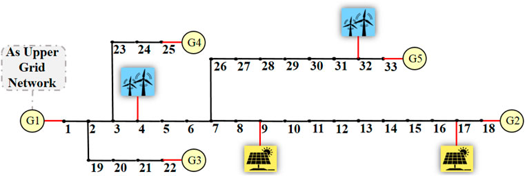
Figure 2. The enhanced IEEE 33-bus distribution system.

Table 1

Table 1. Parameters of the enhanced IEEE 33-bus distribution system.

Table 2

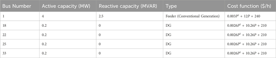
Table 2. Generators data of the enhanced IEEE 33-bus distribution system (Dolatabadi et al., 2020).

Figure 3

Figure 3. The electrical active/reactive load in each bus.

The control of the on- and off-times and the capacity of the HVAC system units are managed by the HVAC aggregator. The specifications of the HVAC system are listed in Table 3. According to the formulas provided in the preceding section and the information in the aforementioned table, the nominal cooling capacity of each unit amounts to approximately 7.1 kW of electricity. By disregarding its heating component and considering the 0.4 MW capacity of the HVAC aggregator, the number of HVAC system units can be computed. The placement of the HVAC aggregator was designated as Bus 8. The performance of the HVAC aggregator was evaluated in both flexible and non-flexible modes. In the nonflexible mode, the input data comprises only the input temperature and ambient conditions. Conversely, in the flexible mode, adjustments are made based not only on the aforementioned factors but also in alignment with the load diagram. The HVAC aggregator is well versed in the permissible operating temperature range of the HVAC system units, set between 18° and 22°, as per the projected load curve of the system for the upcoming hours. Consequently, to curtail electricity consumption during peak load periods and optimize utilization during off-peak and valley periods to offset the required power, it operates in accordance with the DR. The following are depicted in Figure 4: a) inlet temperature and ambient conditions at the preceding moment, b) variations in the current inlet temperature in both flexible and non-flexible modes, and c) electricity consumption of each unit within the HVAC aggregator in the aforementioned modes. Notably, the flexible mode shows a reduction in electricity consumption during peak hours, with a subsequent shift towards off-peak and valley periods.

Table 3

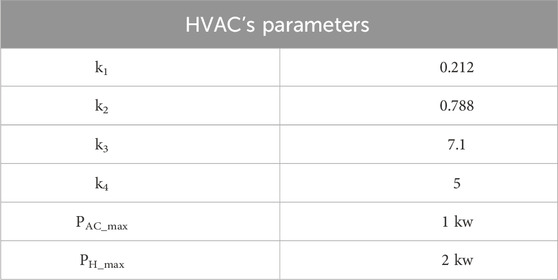
Table 3. The characteristics of a single HVAC (Makhdoomi and Moshtagh, 2023).

Figure 4

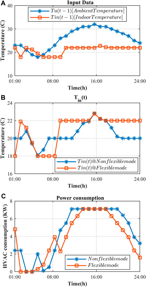
Figure 4. Flexible and non-flexible mode for HVAC unit: (A) input data, including ambient and indoor temperature at (t-1), (B) indoor temperature at (t), (C) power consumption of HVAC units.

In order to calculate the size and number of ESS in distribution system, parameter in Table 4 are considered. The optimal allocation of ESS units in IEEE 33 bus distribution network is depicted in Figure 5. The ESS was placed to reduce the cost of the entire system. After allocating ESS units in the smart distribution grid, the study focuses on achieving the desired objective function through DR calculations within the AC-OPF framework. Due to the nonlinearity of the problem and integer variables, the GAMS software with Mixed-Integer Nonlinear Programming (MINLP) was used to model the issue, and CONOPT3 was employed as a high-speed MINLP solver for large-scale problems. The research was conducted on a PC with an Intel Core i7 processor, 2.2 GHz CPU, and 6 GB of RAM.

Table 4

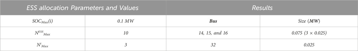
Table 4. The ESS allocation parameters and results.

Figure 5

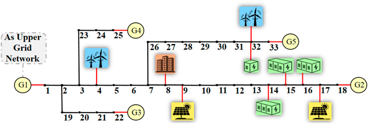
Figure 5. The optimal allocation of ESS units in IEEE 33 bus distribution network.

3.1 Uncertainty of Distributed Energy Resources

The uncertainties mainly arise from random variations in the input data, prediction errors, network failures, and intermittent behavior of RESs. In such an uncertain environment, deterministic power flow (DPF) is infeasible and cannot precisely reveal the state of the system. Therefore, for uncertainty assessment, several uncertainty modeling techniques exist, such as probabilistic approaches, possibilistic approaches, hybrid probabilistic-possibilistic approaches, information gap decision theory (IGDT), interval analysis, and robust optimization (Singh et al., 2022). One of the possibilistic methods is scenario-based. Although the scenario-based method has disadvantages such as sensitivity to selected scenarios and complexity in the number of scenarios, advantages such as flexibility and the possibility of performing sensitivity analysis have led to the use of this method. The three scenarios of normal, high, and low production for each solar and wind unit are shown in Figure 6. Each of these three scenarios was assigned a probability of occurrence in such a way that for the three scenarios of normal, high, and low production in the wind system, the probability of occurrence is 50, 25, and 25, and in the solar system, it is 60, 20%, and 20%, respectively. Owing to the existence of three scenarios for each of the sources, and without losing the generality of the problem, nine scenarios were obtained, and their probabilities are depicted in Figure 7. In each of the nine scenarios, the problem was solved and multiplied by the probability of its occurrence, and the system output was obtained from the sum of the results of the nine scenarios, taking into account the uncertainty of scattered production resources.

Figure 6

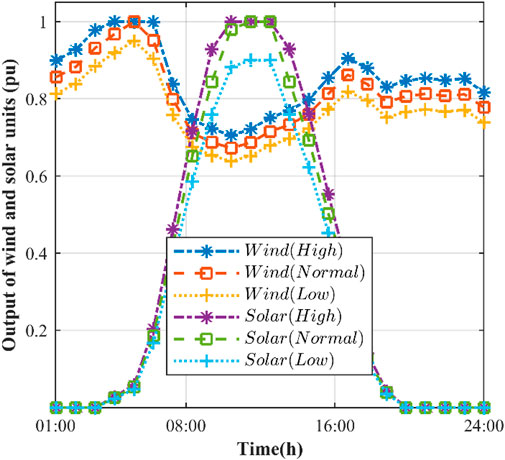
Figure 6. Uncertainty scenarios of wind and solar units.

Figure 7

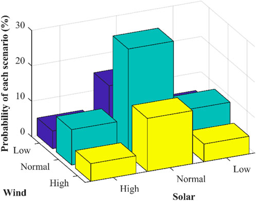
Figure 7. Probability of each scenario for distributed energy resources.

3.2 Demand prediction

Accurate electricity demand prediction is vital for efficient network operation because errors can result in increased production costs and grid losses. Also seasonal ARIMA has better forecasting result for capturing the seasonality and short-term fluctuations in demand but in general, LSTM performed better for products with stable demand (Falatouri et al., 2022). In this study, the Modified LSTM method for load predictions, based on the deep neural network architecture referenced in (Zarei and Ghaffarzadeh, 2023), was utilized. The prediction data cover the period from August 19 to 19 September 2022, and were obtained from the New Zealand Electricity Company (Live load data, 2022) using the MATLAB software. Figure 8 demonstrates the load prediction using this method, with the achieved accuracy indicated by the root-mean-square error and mean absolute error values of 61.8 and 274.9, respectively.

Figure 8

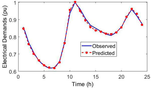
Figure 8. Modified LSTM load prediction.

4 Results and discussion

This section compares the performance of the proposed DR-based AC-OPF in various states and investigates the effect of the HVAC aggregator on peak reduction, various RES scenarios on total cost, DR on voltage profile, peak reduction, and valley filling, and finally, an analytical multi-objective optimization analysis.

4.1 Investigating the effect HVAC aggregator

Two flexible and non-flexible modes were considered for the aggregator to investigate the effect of the HVAC aggregator on DR. As mentioned earlier, this aggregator is included in Bus 8 with a capacity of 0.4 megawatts and a power factor of 0.8. In flexible mode, the aggregator adjusts its performance according to the predicted load chart. In addition to the ambient temperature inside and outside the building, it also checks the load chart and then makes a decision regarding the settings of the on and off times and the corresponding power. For a better comparison, in addition to the simultaneous effect of flexible aggregators and non-flexible, different percentages of DR were applied to other buses. In Figures 9–12, respectively, the objective functions of the total cost, total voltage variation, peak reconnection, and use convenience are displayed in two different modes of aggregator operation and in different DR steps. As can be seen in all the different DRs, the total system cost and total voltage variation in the flexible operating mode of the HVAC aggregator are reduced, and the amount of peak reduction also increases in this mode. The aggregator installed at a point does not have a noticeable effect on the fourth objective function, that is, the UC. To investigate the effect of the HVAC aggregator individually, in the state without DR, the demand of the entire network in two flexible and nonflexible modes is shown in Figure 13. Because its capacity is approximately 10% of the demand of the entire system, a noticeable reduction in the two peak loads and the transfer of its consumption time to periods of low and intermediate loads are observed.

Figure 9

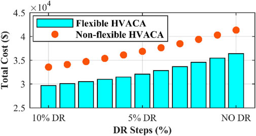
Figure 9. The comparison of total cost in different cases.

Figure 10

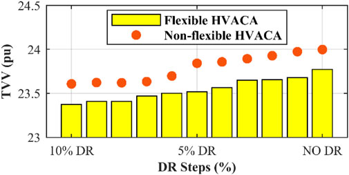
Figure 10. The comparison of TVV in different cases.

Figure 11

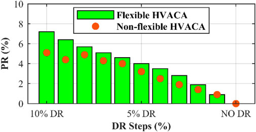
Figure 11. The comparison of peak reduction in different cases.

Figure 12

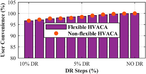
Figure 12. The comparison of UC in different cases.

Figure 13

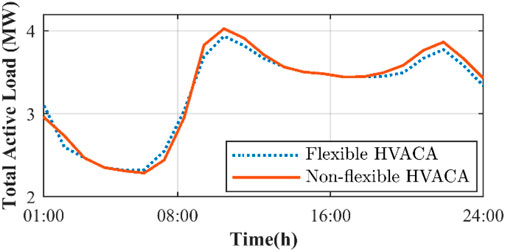
Figure 13. Flexible and non-flexible HVAC aggregator effect on total demand (with no DR).

4.2 Effect of different RES scenarios on total cost of grid

According to the possible scenarios for RESs, the total cost of the system in different DRs from zero to 10% is calculated and shown in Figure 14. Therefore, in scenarios with the possibility of producing more energy through solar and wind energy, the cost of the entire system is reduced. In addition, the cost of the entire system decreased significantly with an increase in the DR. Scenario 9, characterized by maximum solar and wind production, exhibits the lowest cost at each DR step, whereas Scenario 5, with minimal renewable resource production, incurs the highest system cost.

Figure 14

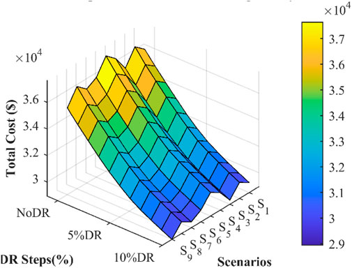
Figure 14. The total cost comparison in various DR steps for the all scenarios.

4.3 Demand response effect on voltage profile

In Figure 15, the voltages of all buses are shown under peak load and low load conditions, with and without consideration of the DR. As can be seen, the effect of applying the DR is to improve the voltage of all buses and approach the optimal voltage (1 pu), especially in low load and end buses of the distribution network.

Figure 15

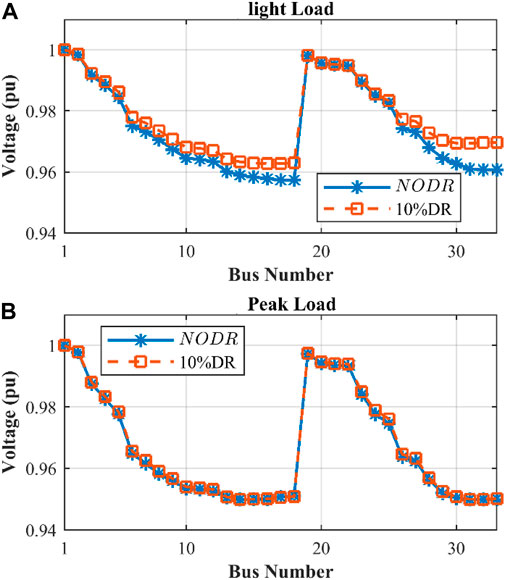
Figure 15. Voltage profile of buses in a modified IEEE 33-bus system for: (A) without DR, (B) 10% DR.

4.4 Demand response effect on peak reduction and valley filling

The effect of levelization on the demand graph of all network loads by applying DR is presented in Figure 16. In the case without DR, the load curve had a desert valley and almost two afternoon and evening peaks. By applying only 10% DR, valley filling has been done to a considerable extent, and almost all the two peaks mentioned have also had a significant reduction. This important factor causes fewer negative effects on the smart distribution grid during peak times.

Figure 16

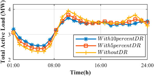
Figure 16. Peak reduction in demand response program.

4.5 Demand response effect on load scheduling

In this subsection, the load scheduling involving demand response at various generating stations, including conventional, wind, solar, DG, and ESS, is discussed. Additionally, the electrical load power, including electrical load and power loss, is presented both without DR and with 10% DR states. As depicted in Figure 17, the implementation of a 10% DR results in a reduction of conventional generation and a subsequent decrease in generation costs. Furthermore, with the 10% DR, power generation costs are lower at lower loads, leading to an increase in power generation by DGs compared to scenarios without demand response.

Figure 17

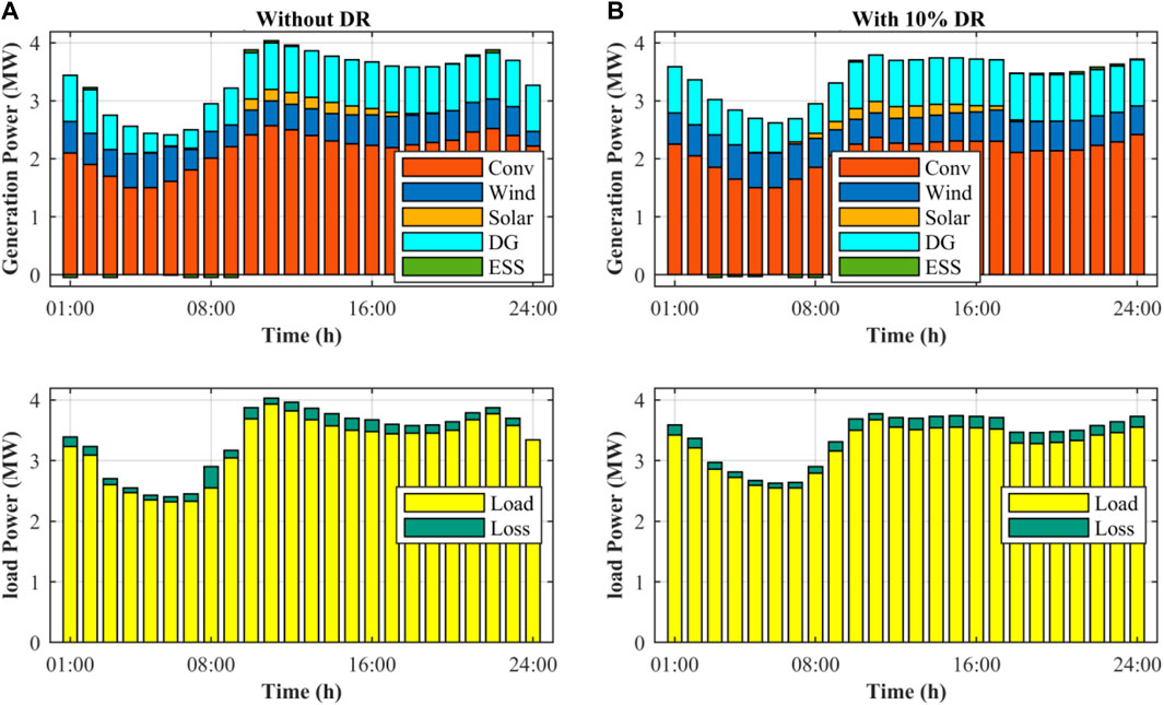
Figure 17. The effect of DR program on generation scheduling: (A) Without DR and (B) with 10% DR.

4.6 Multi-objective optimization analysis

In order to address multi-objective optimization challenges, various methods like the Ɛ-Constraint and TOPSIS are utilized. Each method has its own set of advantages and drawbacks. Figure 18 illustrates the values of four objective functions: total cost (TC), total voltage variation (TVV) for power quality enhancement, peak reduction (PR), and user convenience (UC), ranging from 0 to 30 percent of DR. Utilizing the TOPSIS method identified the optimal point in DR at 30%, albeit resulting in a significant decrease in user convenience from 100% to nearly zero. Given the opposing trends of the other three functions in comparison with UC, even with low weighting factors, the final solution remains unaffected. To address this issue, a thorough analytical approach to the objective function responses is imperative. The cost function exhibited a fully decreasing trend, with a steeper decline at lower DR values and a more gradual decrease at higher DR values. The TVV objective function displays a slight decrease with increasing DR, with a reduction range of less than 0.7% between 23.7 and 23. Because a substantial reduction in TVV comes at a high cost, a balance must be struck. Peak reduction, as the third objective, sees a rapid increase in peak value at the start of DR, reaching a local peak of over 10% before 15% DR, followed by minimal changes thereafter, and maintaining peak reduction below 12% up to DR 30%. Despite increasing the DR in certain regions, a decrease in the PR may still occur. Finally, the UC objective function focuses on user convenience, which diminishes gradually with DR, drops sharply after 15% DR, and approaches zero at 30% DR. Considering the explanations provided, the importance of subscriber consumption patterns, and the societal impact of economic decisions, an analytical approach suggests that DR values below 15% are optimal for altering subscriber consumption patterns. During this phase, when UC falls below 20%, significant cost reductions across the system and optimal peak efficiency are achieved at a DR of 14%.

Figure 18

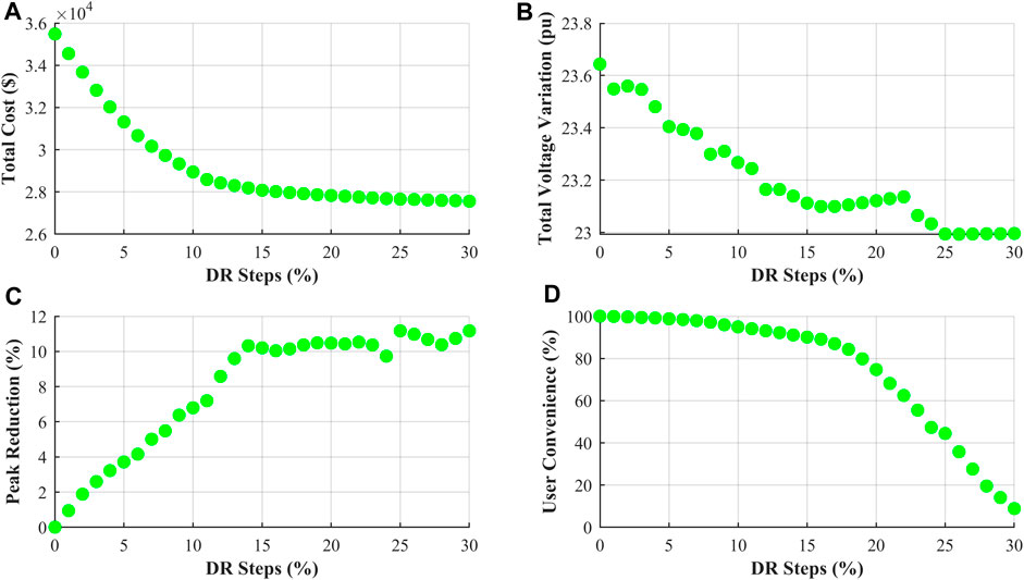
Figure 18. Multi-objective optimization results and analysis.

4.7 Practical implications

The simultaneous solution of AC-OPF and DR problems in a smart distribution network was achieved by applying the effects of a small-scale load aggregator owing to its control and feedback capabilities. Although, in theory, there is no limit to the participation of more electricity subscribers in demand response, in practice, a large change in the time and amount of their consumption will cause dissatisfaction. In practice, choosing the appropriate percentage of DR by considering the behavioral habits of energy consumption of electricity subscribers in the framework of user convenience makes the network operator’s planning on this value closer to reality and reduces the difficulty of adjusting the demand-production balance. The participation of the local aggregator of the HVAC loads to comply with the optimal temperature range of the residents was also emphasized.

5 Conclusion

The integration of renewable energy sources with their intermittent operation and unbalanced electrical loads has created challenges for power grids, particularly in the distribution network section. This paper presents a multi-objective DR approach within the AC-OPF framework by employing two simultaneous participation options: distributed flexible and concentrated aggregated loads. The simulation results demonstrate that flexible modeling of the HVAC aggregator, considering the optimal temperature range for the operation of the units, reduces the total cost, peak load, and total voltage variation. By incorporating modified LSTM demand prediction, optimal ESS placement, and addressing the uncertainty in DERs, along with implementing an analytical method and introducing a 15% maximum step in the DR with a negligible impact of less than 10% on user convenience, significant reductions were achieved across various objective functions. Specifically, the total system cost, network peak, and total voltage variation decrease by 22%, 10%, and 2%, respectively. This optimization effort led to a $8,000 cost reduction and a 0.4 MW decrease in peak load. For future work, the electrical power losses can be considered as another objective functions. And more scenarios can be used for more exact uncertainty modelling of DERs.

Data availability statement

The original contributions presented in the study are included in the article/Supplementary material, further inquiries can be directed to the corresponding author.

Author contributions

AZ: Conceptualization, Formal Analysis, Methodology, Resources, Software, Validation, Visualization, Writing–original draft. NG: Conceptualization, Data curation, Investigation, Project administration, Supervision, Validation, Writing–review and editing. FS: Resoures, Validation, Writing–review and editing.

Funding

The author(s) declare that no financial support was received for the research, authorship, and/or publication of this article.

Conflict of interest

The authors declare that the research was conducted in the absence of any commercial or financial relationships that could be construed as a potential conflict of interest.

Publisher’s note

All claims expressed in this article are solely those of the authors and do not necessarily represent those of their affiliated organizations, or those of the publisher, the editors and the reviewers. Any product that may be evaluated in this article, or claim that may be made by its manufacturer, is not guaranteed or endorsed by the publisher.

References

2011 Buildings energy data Book, energy efficiency and renewable energy: building of technologies program. U.S. Department of Energy, Washington, DC,

Google Scholar

Aalami, H. A., Moghaddam, M. P., and Yousefi, G. R. (2010). Modeling and prioritizing demand response programs in power markets. Electr. power Syst. Res. 80 (4), 426–435. doi:10.1016/j.epsr.2009.10.007

CrossRef Full Text | Google Scholar

Albadi, M. H., and El-Saadany, E. F. (2008). A summary of demand response in electricity markets. Electr. power Syst. Res. 78 (11), 1989–1996. doi:10.1016/j.epsr.2008.04.002

CrossRef Full Text | Google Scholar

Bhattacharya, S., Kar, K., and Chow, J. H. (2017). Optimal precooling of thermostatic loads under time-varying electricity prices. Proc. Am. Control Conf., 1407–1412. doi:10.23919/ACC.2017.7963150

CrossRef Full Text | Google Scholar

Cain, M. B., O’neill, R. P., and Castillo, A. (2012). History of optimal power flow and formulations. Fed. Energy Regul. Comm. 1, 1–36.

Google Scholar

Chowdhury, M. M.-U.-T., Biswas, B. D., and Kamalasadan, S. (2023). Second-order cone programming (SOCP) model for three phase optimal power flow (OPF) in active distribution networks. IEEE Trans. Smart Grid 14, 3732–3743. doi:10.1109/tsg.2023.3241216

CrossRef Full Text | Google Scholar

Dolatabadi, S. H., Ghorbanian, M., Siano, P., and Hatziargyriou, N. D. (2020). An enhanced IEEE 33 bus benchmark test system for distribution system studies. IEEE Trans. Power Syst. 36 (3), 2565–2572. doi:10.1109/tpwrs.2020.3038030

CrossRef Full Text | Google Scholar

Falatouri, T., Darbanian, F., Brandtner, P., and Udokwu, C. (2022). Predictive analytics for demand forecasting–a comparison of SARIMA and LSTM in retail SCM. Procedia Comput. Sci. 200, 993–1003. doi:10.1016/j.procs.2022.01.298

CrossRef Full Text | Google Scholar

Gorman, W. (2022). The quest to quantify the value of lost load: a critical review of the economics of power outages. Electr. J. 35 (8), 107187. doi:10.1016/j.tej.2022.107187

CrossRef Full Text | Google Scholar

Halbhavi, S. B., Karki, S., and Kulkarni, S. G. (2012). Reactive power pricing framework problems and a proposal for a competitive market. Int. J. Innov. Eng. Technol. 1 (2), 22–27.

Google Scholar

Henríquez, R., Wenzel, G., Olivares, D. E., and Negrete-Pincetic, M. (2017). Participation of demand response aggregators in electricity markets: optimal portfolio management. IEEE Trans. Smart Grid 9 (5), 4861–4871. doi:10.1109/tsg.2017.2673783

CrossRef Full Text | Google Scholar

Jabari, F., Mohammadpourfard, M., and Mohammadi-Ivatloo, B., “AC optimal power flow incorporating demand-side management strategy,” in Demand Response Appl. Smart Grids Operation Issues-Volume 2, 2020, pp. 147–165. doi:10.1007/978-3-030-32104-8_7

CrossRef Full Text | Google Scholar

Khonji, M., Chau, C.-K., and Elbassioni, K. (2016). Optimal power flow with inelastic demands for demand response in radial distribution networks. IEEE Trans. Control Netw. 5 (1), 513–524. doi:10.1109/tcns.2016.2622362

CrossRef Full Text | Google Scholar

Li, B., Wan, C., Li, Y., Jiang, Y., and Yu, P. (2023). Generalized linear-constrained optimal power flow for distribution networks. IET Gener. Transm. Distrib. 17, 1298–1309. doi:10.1049/gtd2.12735

CrossRef Full Text | Google Scholar

Live load data (2022). Live load data. Available at: https://www.transpower.co.nz/system-operator/operational-information/load-graphs#download.

Google Scholar

Mak, T. W. K., Chatzos, M., Tanneau, M., and Van Hentenryck, P. (2023). Learning regionally decentralized ac optimal power flows with admm. IEEE Trans. Smart Grid 14, 4863–4876. doi:10.1109/tsg.2023.3251292

CrossRef Full Text | Google Scholar

Makhdoomi, H., and Moshtagh, J. (2023). Optimal scheduling of electrical storage system and flexible loads to participate in energy and flexible ramping product markets. J. Oper. Autom. Power Eng. 11 (3), 203–212. doi:10.22098/joape.2023.10258.1729

CrossRef Full Text | Google Scholar

Merrad, Y., Habaebi, M. H., Toha, S. F., Islam, M. R., Gunawan, T. S., and Mesri, M. (2022). Fully decentralized, cost-effective energy demand response management system with a smart contracts-based optimal power flow solution for smart grids. Energies 15 (12), 4461. doi:10.3390/en15124461

CrossRef Full Text | Google Scholar

Nair, A. S., Abhyankar, S., Peles, S., and Ranganathan, P. (2022). Computational and numerical analysis of ac optimal power flow formulations on large-scale power grids. Electr. Power Syst. Res. 202, 107594. doi:10.1016/j.epsr.2021.107594

CrossRef Full Text | Google Scholar

Nakabi, T. A., and Toivanen, P. (2021). Deep reinforcement learning for energy management in a microgrid with flexible demand. Sustain. Energy , Grids Netw. 25, 100413. doi:10.1016/j.segan.2020.100413

CrossRef Full Text | Google Scholar

Nan, S., Zhou, M., and Li, G. (2017). Optimal residential community demand response scheduling in smart grid. Appl. Energy 210, 1280–1289. doi:10.1016/j.apenergy.2017.06.066

CrossRef Full Text | Google Scholar

Shoreh, M. H., Siano, P., Shafie-khah, M., Loia, V., and Catalão, J. P. S. (2016). A survey of industrial applications of Demand Response. Electr. Power Syst. Res. 141, 31–49. doi:10.1016/j.epsr.2016.07.008

CrossRef Full Text | Google Scholar

Singh, V., Moger, T., and Jena, D. (2022). Uncertainty handling techniques in power systems: a critical review. Electr. Power Syst. Res. 203, 107633. doi:10.1016/j.epsr.2021.107633

CrossRef Full Text | Google Scholar

Soroudi, A. (2017) Power system optimization modeling in GAMS.

Google Scholar

Thanh, V.-V., Su, W., and Wang, B. (2022). Optimal DC microgrid operation with model predictive control-based voltage-dependent demand response and optimal battery dispatch. Energies 15 (6), 2140. doi:10.3390/en15062140

CrossRef Full Text | Google Scholar

Vanin, M., Van Acker, T., Ergun, H., D’hulst, R., Vanthournout, K., and Van Hertem, D. (2022). Congestion mitigation in unbalanced residential networks with OPF-based demand management. Sustain. Energy, Grids Netw. 32, 100936. doi:10.1016/j.segan.2022.100936

CrossRef Full Text | Google Scholar

Wang, J., Xu, Q., Su, H., and Fang, K. (2021). A distributed and robust optimal scheduling model for an active distribution network with load aggregators. Front. Energy Res. 9, 646869. doi:10.3389/fenrg.2021.646869

CrossRef Full Text | Google Scholar

Wolgast, T., Ferenz, S., and Nieße, A. (2022). Reactive power markets: a review. IEEE Access 10, 28397–28410. doi:10.1109/access.2022.3141235

CrossRef Full Text | Google Scholar

Younesi, A., Wang, Z., and Siano, P. (2024). Enhancing the resilience of zero-carbon energy communities: leveraging network reconfiguration and effective load carrying capability quantification. J. Clean. Prod. 434, 139794. doi:10.1016/j.jclepro.2023.139794

CrossRef Full Text | Google Scholar

Zarei, A., and Ghaffarzadeh, N. (2023). Optimal demand response-based AC OPF over smart grid platform considering solar and wind power plants and ESSs with short-term load forecasts using LSTM. J. Sol. Energy Res. 8 (2), 1367–1379. doi:10.22059/JSER.2023.352567.1271

CrossRef Full Text | Google Scholar

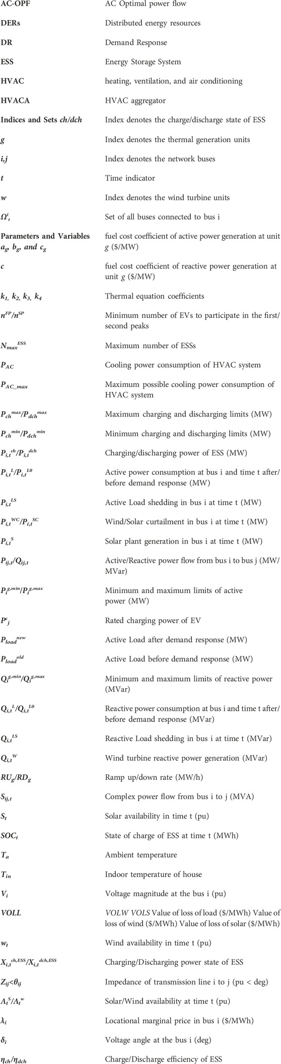
Nomenclature