A study of home energy management considering carbon quota

The household energy management system (HEMS) has become an important system for energy conservation and emission reduction. In this study, home energy management considering carbon quota has been established. Firstly, the household photovoltaic output model, load model of various electrical appliances, battery load model, and charging and discharging of electric vehicles (EVs) model are established. Secondly, the carbon emission and carbon quota of household appliances and EVs are considered in these models. Thirdly, the energy optimization model of minimum the household user’s total comprehensive operation cost with the minimum total electricity consumption, carbon trading cost, battery degradation cost, and carbon quota income are proposed, taking into account constraints such as the comfort of users’ energy use time. Subsequently, the improved particle swarm optimization (IPSO) algorithm is used to tackle the problem. Compared to the standard particle swarm optimization (PSO), the IPSO has significantly improved the optimization effect. By comparing the optimization results in different scenarios, the effectiveness of the strategy is verified, and the influence of different carbon trading prices on optimal energy scheduling has been analyzed. The result shows that the comprehensive consideration of carbon trading cost and total electricity cost can reduce the household carbon emissions and the total electricity cost of the household user. By increasing the carbon trading price, the user’s carbon trading income and the EV carbon quota income increase, and the overall operating cost decreases; the guidance and regulation of carbon trading price can make a valuable contribution to HEMS optimization. Compared to the original situation, the household carbon emissions are reduced by 14.58 kg, a decrease of over 21.47%, while the total comprehensive operation cost are reduced by 14.12%. Carbon quota trading can guide household users to use electricity reasonably, reducing household carbon emissions and the total cost of household electricity.

1 Introduction

With the economy increasing and society developing, carbon emission reduction has become a hot research topic. The proportion of household electricity in economic and social development is gradually increasing, and household energy management is becoming more important. Analyzing users’ electricity consumption habits, adjusting their electricity consumption mode, and realizing energy-saving and low-carbon operation will help to improve power system operation. It is effective in achieving the dual carbon goal on the end user by reducing their electricity consumption cost and carbon emissions.

The studies using home energy management systems (HEMSs) essentially pursue the optimal energy consumption scheme for energy users.

Researchers have focused the optimization problem on various objectives. The objective of many studies is to minimize operation cost (Javadi M S et al., 2020; Lu Q et al., 2020; Sarker E et al., 2020; Thabo G et al., 2021; Ubaid ur Rehman et al., 2022). Sarker E et al. (2020) studied a model of household load management, aiming to minimize the total electricity cost. The response effects of different types of households to price demand with the goal of minimizing cost were analyzed. Javadi M S et al. (2020) proposed an effective HEMS for the self-scheduling of users, and this model considered a dynamic pricing scheme. Lu Q et al. (2020) proposed a model aiming to minimize the peak load and electricity cost to better coordinate household appliances. Thabo G et al. (2021) studied the impact of user’s price and incentive demand response on dynamic economic dispatch and established a multi-objective model considering operating costs and renewable energy penetration. Meanwhile, Marcos Tostado-Véliz et al. (2022) developed a HEMS that incorporates three different strategies of demand response; it also used a novel scenario-based approach. Marcos Tostado-V´eliz et al. (2023) proposed a fully robust model and used it to solve the inherent uncertainties which may arise in home energy management. H. Merdanoglu et al. (2020) focused on optimal appliance power to minimize energy cost. The uncertainties from renewable energy, the end user, and the Real-time Transport Protocol were incorporated into the mixed integer linear programming problem through simple stochastic models. Based on the purpose of reducing electricity charges, the above documents considered the guidance of price and incentive on household energy scheduling, but the user’s comfort requirements and other aspects were not considered.

As mentioned above, these studies ineluctably require users to compromise between electricity costs and comfort. This would inherently change user’s energy comfort. Some researchers have studied the end user’s comfort/discomfort from a multi-objective optimization perspective. A.H. Sharififi et al. (2019) proposed a method that can reduce electricity cost while taking into account the residents’ comfort, and it can improve the peak-to-average ratio. Pamulapati T et al. (2020) established a multi-objective optimization model for intelligent electrical equipment based on economy and comfort. ALIC O et al. (2021) considered the compromise between user cost and comfort goal and analyzed the impact of various electricity prices on user energy management. The above studies considered the comfort of electricity, but the carbon emission cost and carbon trading mechanism of the user were ignored. Li ZK et al. (2020) established a bi-layer optimization model which mainly considered the power station and fully participating householders. Lu Q et al. (2020) aimed to minimize the energy consumption cost and comfort deviation, and it built six modeled by comfort deviation for different kinds of uncertain behaviors.

Optimizing the charging/discharging behaviors of both EVs and energy storage in HEMSs has been widely discussed. Wang S et al. (2020) and Marcos Tostado-V´eliz et al. (2023) studied the cost of battery degradation. Sun C et al. (2016) focused on the economics between lithium-ion battery aging and economic performance in energy management. The battery degradation cost will affect the EVs and energy storage participating in home energy management. To encourage the users to participate in home energy management, a main method is to design a reasonable method for battery degradation costs’ compensation. Wang Y et al. (2020) and Nie Q et al. (2022) thought the carbon trading mechanism is an important way to compensate for the battery degradation cost. Lu Q et al. (2021) proposed a two-level community integrated energy service system optimization model. Gao JW et al. (2021) proposed a comprehensive energy multi-objective scheduling model, which considered the utility of decision makers. The communities’ carbon emissions are taken into account. Tan QL et al. (2019) proposed a model with multiple hybrid energy scheduling for an integrated power system, and it considered five different scheduling modes and a dynamic carbon trading system. Cheng X et al. (2021) built a carbon emission flow model and used it to reduce carbon emissions by carbon trading. These studies on carbon emissions pay close attention to the energy sector, production enterprises, and the community integrated energy, but the end-users in HEMSs are often ignored. This paper will focus on the optimization of the HEMS considering user’s satisfaction and carbon emission.

Ali Abdelrahman O. Ali et al. (2022) have reviewed some optimization schedule methods, which include the mathematical, metaheuristic, and artificial intelligence optimization techniques. Mathematical techniques contain two main groups: linear programming and non-linear programming. Rahima S et al. (2016) conducted a study verifying that the mathematical methods cannot deal with large number of different domestic appliances having unpredictable, non-linear, and complicated energy consumption models. H. Merdanoglu et al. (2020) and El Sayed F. Tantawy et al. (2022) thought heuristic optimization is a strategy intended to solve any problem more efficiently when mathematical approaches are too slow to solve complex problems. Many heuristics optimization scheduling methods are available for HEMS, such as Genetic Algorithm (GA) (Li S et al., 2019; J. Zupan cic et al., 2020; A.H. Sharififi et al., 2019), PSO (Rahima S et al., 2016), and hybrid algorithm A (Ahmad et al., 2017; Z. A. Khan et al., 2019). To avoid the local optimal phenomenon in the solution, improved algorithms are used to quickly solve the model (Rezaee Jordehi A et al., 2019; Zhu J et al., 2019). Shintaro Ikeda et al. (2019) used differential evolution (DE) to apply district energy optimization, and it was proved the method has high potential to provide comprehensive district energy optimization within a realistic computational time. Ima O et al. (2019) proposed an improved enhanced DE for implementing demand response between aggregator and consumer. Its results show that the algorithm is able to optimize energy usage by balancing load scheduling and the contribution of renewable sources while maximizing user comfort and minimizing the peak-to-average ratio. It is clearly justified that heuristic optimization is suitable for HEMSs. The IPSO has been proven to have good performance in terms of computational speed and solution accuracy.

The main contributions of this paper are as follows:

(1) This paper classifies the loads and establishes models for different loads, and the charging/discharging of household batteries (BT) and electric vehicles (EV) are considered. The load working characteristics and power demand are taken as constraints, and the energy consumption time of time-transferable loads is used to represent user satisfaction.

(2) The household user carbon trading cost model and carbon quota income model for EVs are established, and the battery degradation cost is considered. The optimal scheduling model of the HEMS is formed which aims to minimize the total electricity cost and carbon trading cost, while obtaining the EV carbon quota income of household users. It explores the allocation of household energy and EV carbon.

(3) The IPSO algorithm is used; several scenarios are designed in the calculation examples and the sensitiveness of carbon trading price is analyzed. When carbon trading is considered, the system obtains the carbon quota income, the comprehensive total cost is reduced without carbon trading, and its carbon emissions are also reduced.

The rest of the paper is as follows: Section 2 introduces the HEMS framework; Section 3 constructs the load model; Section 4 establishes the household energy scheduling model considering electricity price, user’s energy consumption time, carbon quota mechanism, and battery degradation; in Section 5, the IPSO is used to solve the problem. In Section 6, examples are given. The household user’s energy management objective under fixed carbon trading price and changing carbon trading price on dispatching are analyzed. Section 7 gives some conclusions.

2 The HEMS framework

The HEMS is supported by advanced measurement monitoring and control technology, a bidirectional communication network, and artificial intelligence technology. The composition for the HEMS is shown in Figure 1. It shows the proposed HEMS integrates the photovoltaic power, household electricity load, and BT.

FIGURE 1

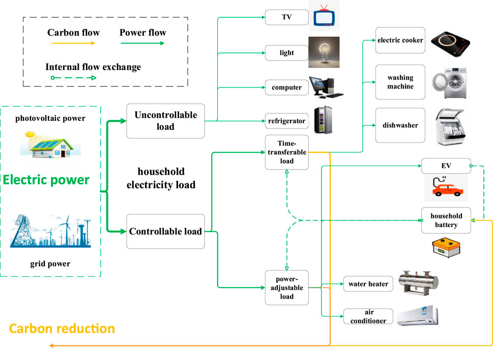
FIGURE 1. HEMS structure.

For the effective dispatch of the household electricity load, this study has classified the load into two categories: uncontrollable load and controllable load. The uncontrollable load covers all necessary appliances (e.g., light, television (TV), computer, and refrigerator). Because of the user’s habits with these appliances, these devices can acquire power at any time without interruption.

The other category is controllable load, including time-transferable load and power-adjustable load. The power-adjustable loads (e.g., EV, water heater, and air conditioner) are scheduled with the user’s preferences. For the time-transferable load, it includes the electric cooker, washing machine, dishwasher, etc. Based on the reasonable electricity price and corresponding constraints, the HEMS can execute the optimal scheduling for the time-transferable loads.

This model contains the time of use pricing, photovoltaic power, and the demand of household electricity loads considering consumer personal preferences. This paper mainly focuses on the energy management and carbon trading of the HEMS, the HEMS structure is shown in Figure 1. The purpose of the HEMS is to reduce the electricity cost, satisfy the electricity needs, and reduce the carbon emissions for household users, and it can also assist in peak load shifting.

3 Load modeling

The usage status of the uncontrollable load has a huge impact on normal life. The time-transferable load will not be interrupted during the whole operation time, the power consumption of such loads generally accounts for a large proportion, and consumers can transfer such loads from peak hours to other periods based on electricity price or the users’ preference. The power-adjustable load can be switched on and off under the condition of meeting the basic working hours, and the power can be adjusted according to the demand.

3.1 Power-adjustable load model

$\left\{\begin{array}{c}{p}_i\left(t\right)=p_i^N\times u_i\left(t\right)\\ u_i\left(t\right)=0,t\in \left[1,24\right]\cup t\notin \left[{\alpha }_i,{\beta }_i\right]\\ {\displaystyle {\sum }_{t={\alpha }_i}^{t={\beta }_i}}{u}_i\left(t\right)=H_i\\ {\alpha }_i<t<{\beta }_i,{\alpha }_i-{\beta }_i\ge H_i\end{array}\right.(1)$

As shown in Eq. 1, where $i$ denotes power-adjustable load, $p_i\left(t\right)$ is the power consumed by power-adjustable load $i$ at time $t$, and $p_i^N$ is the nominal power of power-adjustable load $i$. The $u_i\left(t\right)$ is the status of load $i$ at time $t$, where 0 is off and 1 is on; ${\alpha }_i$ and ${\beta }_i$ are the working time range for power-adjustable load $i$; and $H_i$ is the duration time of load $i$.

Air conditioners, water heaters, household batteries, and EVs are power-adjustable loads. Air conditioners have two states, cooling and heating, and its load models are as follows Eqs 2–6:

$u_{AC,C}\left(t\right)=\left\{\begin{array}{c}1,T_{AC,C,S}+\Delta T_{AC,C}<T^{in}\left(t\right)\\ u_{AC,C}\left(t-1\right),T_{AC,C,S}<T^{in}\left(t\right)\le T_{AC,C,S}+\Delta T_{AC,C}\\ 0,T^{in}\left(t\right)\le T_{AC,C,S}\end{array}\right.(2)$

$H_C={\displaystyle {\sum }_{t=1}^{24}}{u}_{AC,C}\left(t\right)(3)$

$u_{AC,H}\left(t\right)=\left\{\begin{array}{c}1,T_{AC,H,S}+\Delta T_{AC,H}<T^{in}\left(t\right)\\ u_{AC,H}\left(t-1\right),T_{AC,H,S}-\Delta T_{AC,H}<T^{in}\left(t\right)\le T_{AC,H,S}\\ 0,T^{in}\left(t\right)\le T_{AC,H,S}\end{array}\right.(4)$

$H_H={\displaystyle {\sum }_{t=1}^{24}}{u}_{AC,H}\left(t\right)(5)$

$\begin{array}{l}{p}_j\left(t\right)=P_{NC}\times u_{AC,C}\left(t\right)\text{refrigeration}\\ p_j\left(t\right)=P_{NH}\times u_{AC,H}\left(t\right)\text{heating}\end{array}(6)$

The relationship between the indoor temperature change and operating power of air condition can be expressed as Eq. 7:

$T^{\text{in}}\left(t\right)=T^{\text{in}}\left(t-1\right)+a\left(T^{\text{out}}\left(t\right)-T^{\text{in}}\left(t-1\right)\right)+bp\left(t\right)(7)$

where $T_{AC,C,S}$ and $T_{AC,H,S}$ are the temperature set in the cooling and heating state of the air conditioner at time t, respectively; $\Delta T_{AC,C}$ and $\Delta T_{AC,H}$ are the room temperature range set in the cooling and heating state of air conditioners, respectively; $T^{\text{in}}\left(t\right)$ is the indoor temperature at time $t$; $T^{\text{out}}\left(t\right)$ is the outdoor temperature at time $t$; $a$ is the influence coefficient of outdoor temperature on indoor temperature; $b$ is the operating coefficient of the air conditioner, where $b<0$ means that the air conditioner operates in the cooling state and $b>0$ means the air conditioner operates in the heating state; and $u_{AC,C}\left(t\right)$ and $u_{AC,H}\left(t\right)$ are the start-stop variable of the air conditioner at time $t$ period, where 0 is stopping and 1 is starting.

The water heater load model is shown in Eq. 8:

$u_{WH}\left(t\right)=\left\{\begin{array}{c}1,T_{WH}\left(t\right)<T_{WH,S}-\Delta T_{WH}\\ u_{WH}\left(t-1\right),T_{WH,S}-\Delta T_{WH}\le T_{WH}\left(t\right)<T_{WH,S}\\ 0,T_{WH,S}\le T_{WH}\left(t\right)\end{array}\right.(8)$

where $T_{WH,s}$ is the water temperature set by the water heater; $\Delta T_{WH}$ is the set range of water temperature; $T_{WH}\left(t\right)$ is the water temperature at time $t$; and $u_{WH}\left(t\right)$ is the start-stop variable of the water heater at time $t$, where 0 is stopping and 1 is starting.

The output model of the BT is shown in Eq. 9:

$\left\{\begin{array}{c}{S}_{OCBT}\left(t\right)=C_{BT,net}\left(t\right)/C_{BT,bct}\\ S_{OCBT}\left(t+1\right)=S_{OCBT}\left(t\right)+p_{BT,c}\left(t\right)\times \Delta t\times {\theta }_{BT,c}/C_{BT,bat}\\ S_{OCBT}\left(t+1\right)=S_{OCBT}\left(t\right)-p_{BT,d}\left(t\right)\times \Delta t\times {\theta }_{BT,d}/C_{BT,bat}\\ 0\le p_{BT,c}\left(t\right)\le p_{BT,c,\mathit{max}}\\ 0\le p_{BT,d}\left(t\right)\le p_{BT,d,\mathit{max}}\\ S_{OCBT,\mathit{min}}\le S_{OCBT}\left(t\right)\le S_{OCBT,\mathit{max}}\\ {\displaystyle {\sum }_{t=1}^T}\left|u_{BT}\left(t+1\right)-u_{BT}\left(t\right)\right|\le {\lambda }_{BT}\\ p_{BT,c}\left(t\right)\times p_{BT,d}\left(t\right)=0\end{array}\right.(9)$

Output model of an EV shown in Eq. 10:

$\left\{\begin{array}{c}{S}_{OCEV}\left(t\right)=\frac{C_{EV,\text{net}}\left(t\right)}{C_{EV,bat}}\\ S_{OCEV}\left(t+1\right)=S_{OCEV}\left(t\right)+p_{EV,c}\left(t\right)\times \Delta t\times \frac{{\theta }_{EV,c}}{C_{EV,\text{bat}}}\\ S_{OCEV}\left(t+1\right)=S_{OCEV}\left(t\right)-p_{EV,d}\left(t\right)\times \Delta t\times \frac{{\theta }_{EV,d}}{C_{EV,batt}}\\ 0\le p_{EV,c}\left(t\right)\le p_{EV,c,\mathit{max}}\\ 0\le p_{EV,d}\left(t\right)\le p_{EV,d,\mathit{max}}\\ S_{OCEV,\mathit{min}}\le S_{OCEV}\left(t\right)\le S_{OCEV,\mathit{max}}\\ {\displaystyle {\sum }_{t=1}^T}\left|u_{EV}\left(t+1\right)-u_{EV}\left(t\right)\right|\le {\lambda }_{EV}\\ p_{EV,c}\left(t\right)\times p_{EV,d}\left(t\right)=0\end{array}\right.(10)$

where $S_{OCBT}\left(t\right)$ and $S_{OCEV}\left(t\right)$ are the BT and EV state of charging (SOC) at time $t$, respectively; $C_{BT,net}\left(t\right)$ and $C_{EV,net}\left(t\right)$ are the remaining battery capacity of the BT and EV at time $t$, respectively; $p_{BT,C}\left(t\right)$ and $p_{BT,d}\left(t\right)$ are the charging and discharging power of the BT at time $t$, respectively; $p_{EV,c}\left(t\right)$ and $p_{EV,d}\left(t\right)$ are the EV charging and discharging power at time $t$, respectively; ${\theta }_{BT,c}$ and ${\theta }_{BT,d}$ are the BT charging and discharging efficiency, respectively; ${\theta }_{EV,c}$ and ${\theta }_{EV,d}$ are the EV charging and discharging efficiency, respectively; $P_{BT,c,\mathit{max}}$ and ${\mathrm{P}}_{\text{BT},\mathrm{d},\max }$ are the maximum charging and discharging power of the BT, respectively; ${\mathrm{P}}_{\text{EV},\mathrm{c},\max }$ and ${\mathrm{P}}_{\text{EV},\mathrm{d},\max }$ are the maximum charging and discharging power of the EV, respectively; $S_{OCBT,\mathit{max}}$ and $S_{OCBT,\mathit{min}}$ are the maximum and minimum charge state value of the BT, respectively; $S_{OCEV,\mathit{max}}$ and $S_{OCEV,\mathit{min}}$ are the maximum and minimum SOC value of the EV, respectively; $u_{BT}\left(t\right)$ and $u_{EV}\left(t\right)$ are the charging and discharging variables of the BT and EV at time $t,\text{respectively}$, where the value is 0 or 1; and ${\mathrm{\lambda }}_{\text{BT}}$ and ${\lambda }_{EV}$ are limit of charging and discharging times of the BT and EV, respectively.

3.2 Time-transferable load

The time-transferable load has the delayed start function, which can transfer the working interval but cannot reduce the load. The startup and running time can be flexibly set according to the needs of users.

$\left\{\begin{array}{c}{p}_j\left(t\right)=p_j^N\ast u_j\left(t\right)\\ u_i\left(t\right)=0,t\in \left[1,24\right]\cup t\notin \left[{\alpha }_j,{\beta }_j\right]\\ {\displaystyle {\sum }_{t=t_j^{\text{start}}}^{t_j^{\text{end}}}}{u}_j\left(t\right)={\displaystyle {\sum }_{t={\alpha }_j}^{{\beta }_j}}{u}_j\left(t\right)=H_j\\ t_j^{\text{end}}-t_j^{\text{start}}+1=H_j\\ {\alpha }_j\le t_j^{\text{start}}\le t\le t_j^{end}\le {\beta }_j\\ {\beta }_j-{\alpha }_j\ge H_j\end{array}\right.(11)$

As shown in Eq. 11, where $j$ denotes the time-transferable load; $p_j\left(t\right)$ is the electricity power of the time-transferable load $j$ at time $t$; ${\mathrm{p}}_{\mathrm{j}}^{\mathrm{N}}$ is the rated power of time-transferable load $j$; $u_j\left(t\right)$ is start-variable 0–1, where 1 represents the operation of time-transferable load $j$ and 0 indicates the time-transferable load is off; ${\mathrm{\alpha }}_{\mathrm{j}}$ and ${\beta }_j$ are the time-transferable load $j$ allowable start and stop time of operation, respectively; $t_j^{start}$ and $t_j^{end}$ are the time-transferable load $j$ start and end time of actual operation, respectively; and $H_j$ is duration over which time-transferable load $j$ needs to work.

3.3 Uncontrollable load

The uncontrollable load scheduling model is shown in Eq. 12:

$u_k\left(t\right)=\left\{\begin{array}{c}0,t\in \left[1,24\right]\cup t\notin \left[{\alpha }_k,{\beta }_k\right]\\ 1,t\in \left[{\alpha }_k,{\beta }_k\right]\end{array}\right.(12)$

where $u_k\left(t\right)$ is the start-stop variable of uncontrollable load k at time $t$, where 0 indicates off; ${\mathrm{\alpha }}_{\mathrm{k}}$ and ${\beta }_k$ are the allowable start and end time of uncontrollable load $k$, respectively.

4 Household energy scheduling model based on time-of-use tariff and carbon quota mechanism

An energy scheduling model is proposed considering the power consumption cost, carbon trading cost, EV carbon quota income, and battery degradation cost.

4.1 Household user electricity cost model

For household users, the electricity purchase cost $C_1$ includes the electricity consumption cost of the uncontrollable load, time-transferable load, and power-adjustable load. A complete dispatching cycle can be divided into $T$ periods, and the household user’s electricity purchase cost $C_1$ can be expressed as Eq. 13:

$C_1=\left({\displaystyle {\sum }_{t=1}^T}E\left(t\right)-p_{v,\text{used}}\left(t\right)\right)\mathit{pr}{i}_b\left(t\right)(13)$

where $\mathit{pr}{i}_b\left(t\right)$ is the time-of-use electricity price at time $t$; $p_{v,\text{used}}\left(t\right)$ is the photovoltaic power consumed by household appliances at time $t$; and $E\left(t\right)$ is the total energy consumption of all appliances at time $t$.

$E_{cc}\left(t\right)={\displaystyle {\sum }_{i=1}^m}{p}_i\left(t\right)u_i\left(t\right)\Delta t(14)$

$E_{cu}\left(t\right)={\displaystyle {\sum }_{j=1}^m}{p}_j\left(t\right)u_j\left(t\right)\Delta t(15)$

$E_{\mathit{un}}\left(t\right)={\displaystyle {\sum }_{k=1}^m}{p}_k\left(t\right)u_k\left(t\right)\Delta t(16)$

$E\left(t\right)=E_{cc}\left(t\right)+E_{cu}\left(t\right)+E_{un}\left(t\right)(17)$

As shown in Eqs 14–17, where $p_i\left(t\right)$, $p_j\left(t\right)$, and $p_k\left(t\right)$ are the power of the power-adjustable load, time-transferable load, and uncontrollable load at time $t$, respectively; $m$, $n$, and $l$ are the number of the corresponding load; $E_{cc}\left(t\right)$, $E_{cu}\left(t\right)$, and $E_{un}\left(t\right)$ are the power consumption of power-adjustable load, time-transferable load and uncontrollable load at time $t$, respectively.

Household user’s profit $C_2$ from selling electricity is shown in Eqs 18–20:

$C_2={\displaystyle {\sum }_{t=1}^T}{p}_g\left(t\right)\mathit{pr}{i}_g\left(t\right)(18)$

$p_g\left(t\right)=p_{v,g}\left(t\right)+p_{EV,d}\left(t\right)(19)$

$p_v\left(t\right)=p_{v,\text{used}}\left(t\right)+p_{v,g}\left(t\right)(20)$

where $p_v\left(t\right)$ is the photovoltaic supply power at time $t$ and $p_{v,g}\left(t\right)$ is the photovoltaic power sold to the grid at time $t$. The $p_g\left(t\right)$ is the power that household users sell electricity to the grid at time $t$; $\mathit{pr}{i}_g\left(t\right)$ is the price that users sell electricity at to the grid at time $t$; and $p_{EV,d}\left(t\right)$ is the discharge power of EV at time $t$.

The total electricity cost $C$ includes electricity purchase cost $C_1$ and profit from selling electricity, as shown in Eq. 21:

$C=C_1-C_2(21)$

4.2 Household user carbon trading cost model

The carbon dioxide emission generated by the household user is shown in Eq. 22:

$Q_c\left(t\right)=E_{th}\left(E_{cc}\left(t\right)+E_{cu}\left(t\right)+E_{un}\left(t\right)-p_v\left(t\right)\right)(22)$

where $Q_c\left(t\right)$ is the carbon dioxide emission generated by the household user’s electricity usage at time $t$, and $E_{th}$ is the carbon emission coefficient.

The amount of carbon emission quota $M_c\left(t\right)$ obtained by household users from external electricity purchase at time $t$ is shown as Eq. 23:

$M_c\left(t\right)=\epsilon \left(E_{cc}\left(t\right)+E_{cu}\left(t\right)+E_{un}\left(t\right)+p_{EV,c}\left(t\right)\right)(23)$

where $\epsilon$ is the carbon emissions quota allocation coefficient.

When the free carbon quota received by households is greater than their actual carbon emissions, household users can sell their excess carbon emissions to gain profits. If the free carbon quota received by household users is less than their actual carbon emissions, household users need to buy the required carbon emissions from the carbon trading market. Therefore, the carbon trading cost of household users at time $t$ is shown as Eq. 24:

$R_{\text{genbon}}\left(t\right)=q_{\text{th}}\left(Q_c\left(t\right)-M_c\left(t\right)\right)(24)$

where $R_{\text{genbon}}\left(t\right)$ is the carbon trading cost of households at time $t$. When $R_{\text{genbon}}\left(t\right)$ is positive, it means households need to spend extra money to buy the required carbon quota; when $R_{\text{genbon}}\left(t\right)$ is negative, it means the income of households that can sell carbon quota. $q_{th}$ is the carbon trading price.

4.3 Carbon quota income model for EV

The carbon quota $M_{EV}\left(t\right)$ obtained by the discharge of an EV at time $t$ is as follows Eqs 25, 26:

$M_{EV}\left(t\right)=\left(p_{EV,c}\left(t\right)-p_{EV,d}\left(t\right)\right)\Delta t{L}_{EV}{E}_{gas}-p_{EV,c}\left(t\right)\beta \left(t\right)\Delta t{E}_{th}+p_{EV,d}\left(t\right)\Delta t{E}_{th}(25)$

$\beta \left(t\right)=\frac{E\left(t\right)-p_v\left(t\right)}{E\left(t\right)}(26)$

where $\Delta t$ is the time step; $M_{EV}\left(t\right)$ is the carbon quota owned by the EV at time $t$; $L_{EV}$ is the distance that 1 kwh EV can travel; $E_{gas}$ is the carbon emission of the fuel-using car driving 1 km; $E_{th}$ is the carbon emission of per output power of thermal power; and $\beta \left(t\right)$ is the proportion of thermal power capacity in EV charging quantity at time $t$, with the proportion of the total thermal power output in the total system output at time $t$ used for calculation.

The carbon quota income $R_{\text{carbon}}\left(t\right)$ that the EV can sell at time $t$ is shown in Eq. 27:

$R_{\text{carbon}}\left(t\right)=q_{ev}{M}_{EV}\left(t\right)(27)$

where $q_{ev}$ is the EV carbon quota price.

4.4 System objective function

Considering the total electricity cost of the household, household user’s carbon trading cost, battery degradation cost, and EV carbon quota income comprehensively, the objective of the HEMS is to minimize the total comprehensive operation cost:

$\mathit{min}F=\mathit{min}\left(C+{\displaystyle {\sum }_T^{t=1}}\left(R_{\text{genbon}}\left(t\right)-R_{\text{carbon}}\left(t\right)+C_{\text{battery}}\left(t\right)\right)\right)(28)$

As shown in Eq. 28, where $C_{\text{battery}}\left(t\right)$ represents the cost of battery degradation in both the EV and the BT.

$C_{\text{battery}}\left(t\right)=\left(c_{\text{bat}}{E}_{\text{bat}}+c_{\mathrm{L}}\right)\times \frac{p_{EV,d}\left(t\right)}{L_{\mathrm{c}}\times E_{\text{bat}}\text{DOD}}(29)$

As shown in Eq. 29, where $c_{\text{bat}}$ is the battery cost (which includes the EV battery and BT); $c_{\mathrm{L}}$ is the labor cost for battery replacement; $E_{\text{bat}}$ represents the battery capacity; $L_{\mathrm{c}}$ is the cycle life of batteries; and $\text{DOD}$ is the discharge depth at $L_{\mathrm{c}}$.

The expected operation time represents the user’s comfort of energy use. Therefore, the energy consumption time of the time-transferable load is used to represent user satisfaction, and its satisfaction constraint is shown in Eq. 30:

$t_j^{\text{start}}\le t\le t_j^{\text{end}}(30)$

During the scheduling process, users need to comply with the following power balance constraints:

$p_{buy}\left(t\right)+p_V\left(t\right)+p_{EV,d}\left(t\right)+p_{BT,d}\left(t\right)=E_{cc}\left(t\right)+E_{cu}\left(t\right)+E_{un}\left(t\right)(31)$

As shown in Eq. 31, where the $p_{buy}\left(t\right)$ is the user’s purchased power at time $t$.

In summary, the objective function is Eq. 28, and the power balance equality constraint is Eq. 31. Other relevant constraints have been given in the corresponding load models above.

5 Optimization of HMES based on IPSO algorithm

For the optimization of the HEMS, it requires a large amount of calculation. Because there are too many variables in the HEMS, heuristic algorithms can tackle these problems efficiently. At present, heuristic algorithms are widely used in related fields such as community and household energy scheduling. Although heuristic algorithms may not ultimately obtain the ideal value, the IPSO algorithms can obtain the optimal solutions that are extremely close to the ideal value.

5.1 IPSO algorithm

During the parameter initialization phase, the standard PSO algorithm initializes particle positions and velocities with random numbers, resulting in suboptimal exploration of the solution space and limited global search capabilities, particularly in constraint optimization scenarios. Furthermore, the standard PSO algorithm is susceptible to premature convergence and loss of diversity, ultimately hindering its ability to attain highly accurate optimal solutions in HEMS optimization contexts.

The IPSO retains the population diversity, and the initial population is within the feasible domain of particles, which improves the quality of the initial population particle solution. The initial moment the particle swarm population is generated as shown in Eq. 32:

$x_{i,\mathit{int}}=L{b}_i+r_{new}\left(U{b}_i-L{b}_i\right)(32)$

where $x_{i,\mathit{int}}$ is the initial particle population of the IPSO; $r_{new}$ are uniform random numbers for the IPSO; $L{b}_i$ is the lower limit of the $i$ th particle solution in the IPSO; and $U{b}_i$ is the upper limit of the $i$ th particle solution in the IPSO algorithm.

After the improvement, the PSO algorithm first compares the fitness value ${Fit}_i$ of each particle with the individual extreme $p_{id}$, and if ${Fit}_i<p_{id}$, $p_{id}$ is replaced with ${Fit}_i$. ${Fit}_i$ is then compared with the global extremum $p_{gd}$, and if ${Fit}_i<p_{gd}$, $p_{gd}$ is replaced with ${Fit}_i$.

At the same time, in order to alleviate the shortcomings of premature convergence and diversity loss in the standard PSO and improve the solvability of the algorithm in constrained optimization problems, the IPSO improves the update of the standard PSO, and the update formula is shown in Eq. 33:

$x_{i,n+1}=x_{i,n}+beta\times \left(p_{id}-x_{i,n}\right)+alpha\times r_{new}\left(U{b}_i-L{b}_i\right)(33)$

where n is the current iteration number, $x_{i,n}$ is the position of the $i$ th population in the IPSO; $beta$ is adaptive coefficient; $alpha$ is convergence factor $p_{id}$ is Individual extremum.

The IPSO algorithm using Eq. 33 can update and be solved during the optimization process, effectively improving the algorithm’s constraint solving ability and enhancing the PSO algorithm’s ability to find the global optimal solution. However, after updating the position of particles in the population, there may be situations where some particles exceed the population constraint boundary, which greatly reduces the efficiency of the algorithm in searching for particles in the feasible domain. The IPSO algorithm improves the above situation by applying a boundary function to the updated particle population, thereby enhancing the efficiency of the algorithm in searching for feasible solutions. The boundary function of the IPSO algorithm is as follows Eq. 34:

$x_{i,n+1}=\left\{\begin{array}{c}Lbi,if{x}_{i,n+1}\le Lbi\\ x_{i,n+1},ifLbi<x_{i,n+1}<Ubi\\ Ubi,if{x}_{i,n+1}\ge Ubi\end{array}\right.(34)$

5.2 DE algorithm

DE has fewer parameters and is relatively simple to calculate, making it widely used in power scheduling problems. The main process of DE can be shown as five parts (Initialization, Mutation, Crossing, Selection, and Termination):

(1) Initialization:

${\mathit{X}}_{i,G}={\left[x_{i1,G},x_{i2,G},\cdots ,x_{iD,G}\right]}^{\mathrm{T}},i=1,2,\cdots ,N_{\mathrm{P}}(35)$

As shown in Eq. 35, where $x_{id,G}$ (d = 1, 2, … , D) is the dth component of ${\mathit{X}}_{i,G}$, which satisfies the constraint condition $x_{i,d}$ ∈ $\left[x_{id,low},x_{id,up}\right]$. The $x_{id,low}$ and $x_{id,up}$ represent the lower and upper limits of the search range, respectively.

(2) Mutation: The most common mutation strategies are as follows Eqs 36–38:

DE/rand1

${\mathit{V}}_{i,G+1}={\mathit{X}}_{r_0,G}+F_i\left({\mathit{X}}_{r_1,G}-{\mathit{X}}_{r_2,G}\right)(36)$

DE/current-to-rand/1

${\mathit{V}}_{i,G+1}={\mathit{X}}_{i,G}+F_i\left({\mathit{X}}_{\text{best},G}-{\mathit{X}}_{i,G}\right)+F_i\left({\mathit{X}}_{r_1,G}-{\mathit{X}}_{r_2,G}\right)(37)$

DE/best/1

${\mathit{V}}_{i,G+1}={\mathit{X}}_{\text{best},G}+F_i\left({\mathit{X}}_{r_1,G}-{\mathit{X}}_{r_2,G}\right)(38)$

where $r_0$, $r_1$, $r_2$ ∈[1,N_P], NP is a random number that is not identical to each other. The ${\mathit{X}}_{r_1,G}$ and ${\mathit{X}}_{r_2,G}$ is the difference of randomly selecting two vectors. The ${\mathit{X}}_{\text{best},G}$ is the optimal individual in the G generation population. The scaling factor is $F_i$.

(3) Crossing:

$u_{ij,G}=\left\{\begin{array}{c}{v}_{ij,G},\text{rand\hspace{0.17em}}\left[0,1\right]⩽P_{{\mathrm{c}}_i}\text{\hspace{0.17em}or\hspace{0.17em}}j=j_{\text{rand}}\\ x_{ij,G}\end{array}\right.(39)$

As shown in Eq. 39, where $P_{{\mathrm{c}}_i}$ represents the probability of crossing, with values ranging from 0 to 1, and $j_{\text{rand}}$ is a random integer on $1,2,\dots ,\mathrm{D}$.

(4) Selection:

${\mathit{X}}_{i,G+1}=\left\{\begin{array}{c}{\mathit{X}}_{i,G},f\left({\mathit{X}}_{i,G}\right)<f\left({\mathit{U}}_{i,G}\right)\\ {\mathit{U}}_{i,G}\end{array}\right.(40)$

As shown in Eq. 40, where ${\mathit{X}}_{i,G+1}$ refers to the parent individual who successfully enters the next-generation after comparison.

(5) Termination: When G reaches G_max, the requirement is met.

5.3 Algorithm comparison

This study assesses the performance of the algorithm by employing the Sphere, Ackley, Rastrigin, and Griewank functions, with an optimal value of 0 for these functions. The pertinent parameters of the test functions are presented in Table 1. Additionally, the DE, PSO, and IPSO methods are concurrently selected for comparison. Figure 3 illustrates the convergence trajectories of these algorithms, each independently solving the functions 500 times in a 100-dimensional space.

TABLE 1

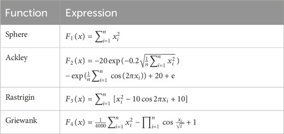
TABLE 1. Function for comparison.

Figure 2 verifies the effectiveness of the IPSO. The IPSO has the best convergence effect compared to PSO and DE, while its final convergence value is closest to the optimal extreme value. The PSO optimization effect is the worst. By adjusting with the introduction of random learning factors, the convergence of the algorithm has been improved.

FIGURE 2

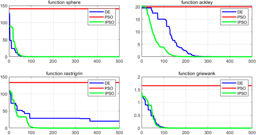
FIGURE 2. Function value convergence curve.

From Table 2, comparing the algorithms in solving complex functions, the IPSO has a faster convergence time than the DE. For the optimization process of the HEMS, a large amount of computing resources is necessary. After comparing the above algorithms, this study selects the IPSO for optimization.

TABLE 2

TABLE 2. Comparison of results.

5.4 The IPSO algorithm process of HEMS

In summary, the IPSO algorithm can enhance computational efficiency and global search capability. The flow chart of the HEMS can be seen in Figure 3. The steps and procedures of the HEMS optimization based on the IPSO algorithm are as follows:

FIGURE 3

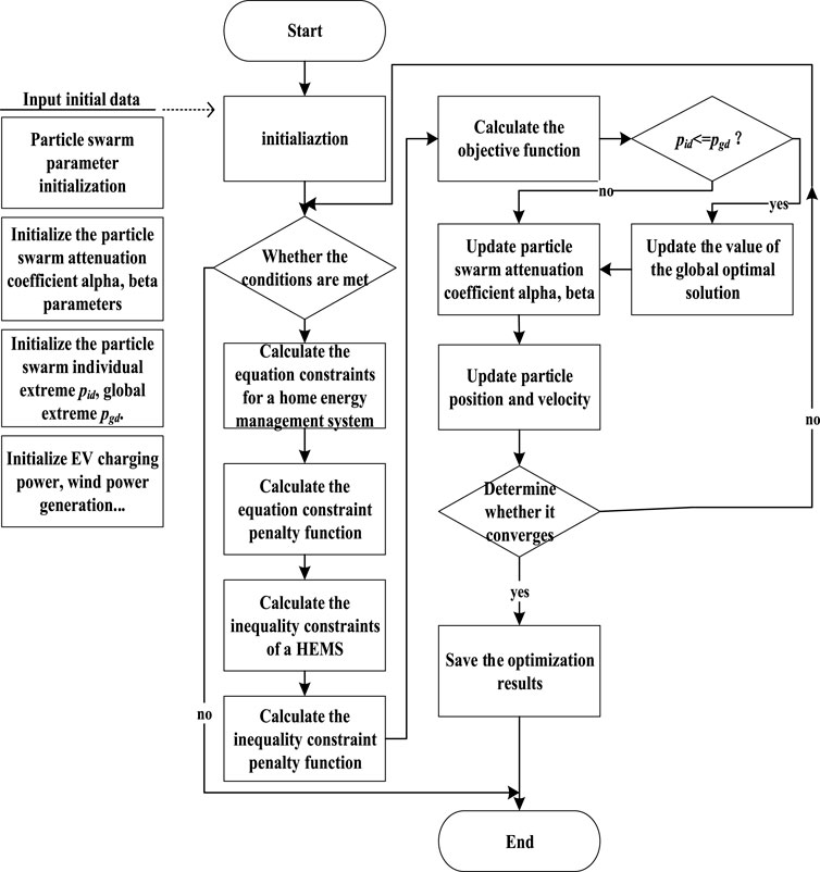
FIGURE 3. The flow chart of the HEMS.

Step 1:. Initialize the EV charging power, wind power generation, etc., as well as the initial parameters of the PSO algorithm such as attenuation coefficient $alpha$, $beta$, individual extremum $p_{id}$, global extremum $p_{gd}$, etc.

Step 2:. Determine whether the time condition and the number of iterations conditions are met. If the conditions are met, proceed to Step 3, otherwise exit the program.

Step 3:. Calculate the medium and inequality constraints of the household energy management system and their penalty functions.

Step 4:. Obtain the objective function value.

Step 5:. If the individual extremum $p_{id}$ is less than or equal to the global extremum $p_{gd}$, the value of the global optimization solution is updated, otherwise Step 4 is returned at the same time.

Step 6:. Update particle swarm attenuation coefficient alpha, beta.

Step 7:. Update the position of the particle according to Eq. 33.

Step 8:. Determine whether the end condition is met, and if so, exit (error reaches set accuracy or reaches the maximum number of cycles), otherwise return to Step 3 to continue the calculation.

6 Case studies

Simulations are given in some cases for the performance of the proposed HEMS model. The scheduling time horizon is 24 h and the scheduling slot is 1 h. The load curve is divided into three different parts: the valley period (from 22:00 to 06:00), when the electricity price is 0.3 CNY/kWh (China yuan/kWh); the off-peak period (from 13:00 to 17:00), when the electricity price is 0.45 CNY/kWh; and the peak period (from 06:00 to 13:00 and from 17:00 to 22:00), when the electricity price is 0.6 CNY/kWh. The discharging of EVd and PV grid price is 0.45 CNY/kWh. The EV battery capacity is 16 kWh, the maximum power of charging/discharging is 1.5 kW, and the charging/discharging efficiencies are 90%. The BT capacity is 10 kWh, the maximum power of charging and discharging is 1 kW, the charge and discharge efficiencies are 90%, and the maximum/minimum state of charge of the EV and BT are 0.9/0.2. When the indoor temperature is higher than 26°C, the air conditioner is turned on; when the temperature is lower than 24°C, it is off. The water heater starts heating while the water temperature is lower than 46°C, and stops heating while the water temperature is higher than 52°C. The electricity consumption of different appliances can be seen in Tables 3, 4. The start-end time of the appliances shows the users’ preferable timings. Other simulation parameters [17] are listed in Table 5. This article uses an IPSO algorithm to solve the problem.

TABLE 3

TABLE 3. Description of time-transferable appliances.

TABLE 4

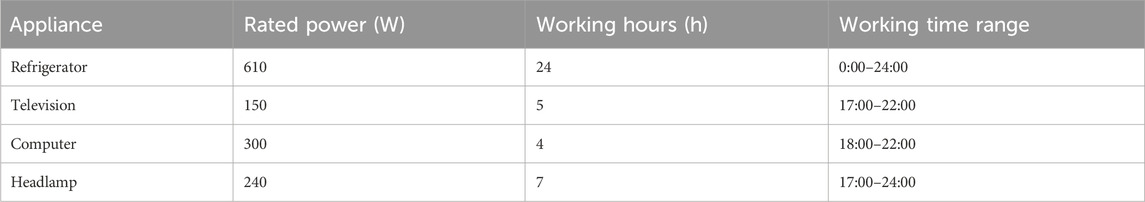
TABLE 4. Description of uncontrollable appliances.

TABLE 5

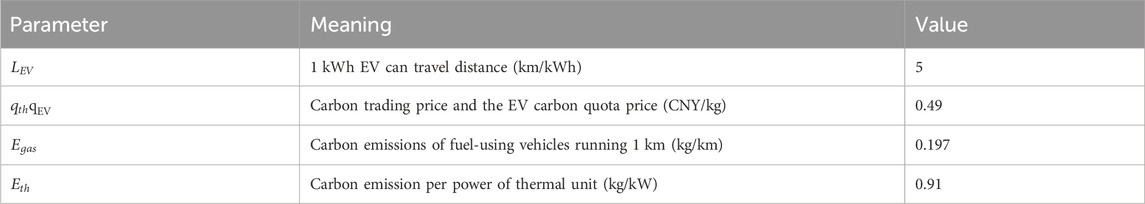
TABLE 5. The related parameters of carbon trading.

6.1 Optimization analysis of household energy under fixed carbon trading price

The following scenarios are set for the comparison of several different schemes:

Scenario 1:. Initial household electricity cost and carbon emissions do not consider optimal scheduling;

Scenario 2:. Optimal scheduling of household energy does not consider carbon trading and time satisfaction;

Scenario 3:. Optimal scheduling of household energy only considers time satisfaction and does not consider carbon trading;

Scenario 4:. Optimal scheduling of household energy only considers carbon trading and does not consider time satisfaction;

Scenario 5:. Optimal scheduling of household energy considering carbon trading and time satisfaction.

Scenario 2, Scenario 3 show that the carbon trading cost of household users and the carbon quota income of EVs are not considered. Scenario 4, Scenario 5 show that the carbon trading cost of household users and the carbon quota income of EVs are considered. Scenario 1 is the initial electricity cost and carbon emissions of households without considering optimal scheduling; in Scenario 2, time satisfaction constraints, user carbon trading costs, and the carbon quota income of EVs are not considered, and the goal is minimizing the total electricity cost; in Scenario 3, carbon trading is not considered, but the time satisfaction constraint is considered, and the total electricity cost is minimized; Scenario 4 considers the user’s carbon trading cost, EV carbon trading income, and the user’s total electricity cost, and the objective is minimizing the user’s comprehensive operation cost, but the time satisfaction constraint is ignored; Scenario 5 considers the user’s total electricity cost, carbon trading cost, and EV carbon trading income, with the objective being minimizing the household user’s comprehensive operating cost with time satisfaction constraints. During the optimization process, the user’s typical daily load in summer is selected as the optimization data.

Figure 4 shows the typical outdoor temperature, the optimized indoor temperature, and the water heater temperature. Figures 5–10 show the power in Scenario 1, Scenario 2, Scenario 3, Scenario 4, Scenario 5.

As shown in Figure 4, the air conditioner remains on, the indoor temperature decreases significantly, and the user’s room can reach the required temperature range. After the water heater is turned on, the water temperature rises to meet the user’s needs.

Figure 5 shows the load comparison between different scenarios. The load increased sharply from 3:00 to 6:00, and the load also increased between 22:00 and 24:00. From 8:00 to 16:00, the load of users decreased sharply. The reason for this was that some of the load was transferred to other periods to reduce the costs.

In Figure 6, the air conditioner has been turned on and the user does not consider the influence of the electricity price on the total household appliances’ cost. When the electricity price is high, the cost of electricity consumption increases accordingly. Discharge of the EV is not used and the charging/discharging behavior of the BT is relatively random. In Figure 7, all electrical appliances run at the lowest electricity price within the allowable time period. Meanwhile, EVs and batteries charge when at low electricity prices and discharge when at high electricity prices. When the photovoltaic output and BT discharge exceed the electricity used by electrical appliances, the user will sell the excess electricity at noon.

In Scenario 1, the electricity cost of the air conditioner is 13.8 CNY; in Scenario 2, the operation time of the air conditioner is significantly reduced, and its electricity cost is 3 CNY and 21.7% less than Scenario 1, and the indoor temperature meets the requirements of the user. The total electricity consumption of the water heater remains unchanged; in Scenario 1, its running time is 19:00 to 22:00 and the electricity cost is 2.7 CNY; in Scenario 2, the running time is 19:00 to 21:00 and 23:00 to 24:00 and the electricity cost is 2.25 CNY and 0.45 CNY, respectively, and 16.7% less than Scenario 1. The user’s water demand is met.

In Scenario 1, the EV is charged between 21:00 and 05:00, and the battery is charged. In Scenario 2, the EV and battery are charged between 23:00 and 07:00, and the electricity cost is 2.25 CNY less than in Scenario 1. In Scenario 1, the EV does not discharge and the BT discharges randomly. In Scenario 2, the discharge of the EV is at 19:00 to 23:00, the BT discharges at 10:00–15:00 and 20:00–23:00, and the electricity cost of the EV and BT is 3.91 CNY less than Scenario 1. The washing machine, rice cooker, dishwasher, vacuum cleaner, and electric kettle all operate during the valley period, when the electricity price is lowest, which significantly cuts the total household electricity cost compared with Scenario 1. However, in Scenario 2, the use of vacuum cleaners is advanced to 5:00, and the use of washing machine and dishwashers is delayed to 23:00, but the user’s usage habits are not considered, resulting in low satisfaction. Compared with Figure 6, considering the time satisfaction of the user with electricity consumption in Scenario 3 of Figure 8, the usage time distribution of the electrical appliances is more reasonable. The vacuum cleaner is transferred from 05:00 to 09:00, the dishwasher changes working time from 23:00 to 21:00, the washing machine changes working time from 23:00 to 17:00, and the electric kettle from 22:00 to 19:00. When the users’ time satisfaction constraint is met, the electricity cost of the time-transferable load is 1.32 CNY more than Scenario 2. In Figures 9, 10, the running conditions of most appliances do not change greatly when carbon trading is considered. In Scenario 4, Scenario 5, carbon trading is considered. The reduction in EV mileage is no less than the increase in the discharge of the EV. Figure 11 gives a comparison of the cost and emissions in each scenario, and the battery degradation cost in each scenario is shown in Table 6.

As shown in Figure 11, compared with Scenario 1, the total comprehensive operation cost and carbon emissions of Scenario 2, Scenario 3, Scenario 4, Scenario 5 have significantly decreased. After considering the time satisfaction constraint in Scenario 3, Scenario 5, compared with Scenario 2, Scenario 4, the electricity purchase cost increases by 1.13 CNY and 0.63 CNY, respectively. In Scenario 4, Scenario 5, when the carbon trading is considered, the system obtains carbon quota income, and the comprehensive total cost is reduced without carbon trading, and its carbon emissions are also reduced. As shown in Table 6, the battery degradation cost in Scenario 1 is much less than it in other scenarios, because EVs do not participate in scheduling, there is no battery degradation cost for EVs, and the overall battery degradation cost for households is lower than in other scenarios.

FIGURE 4

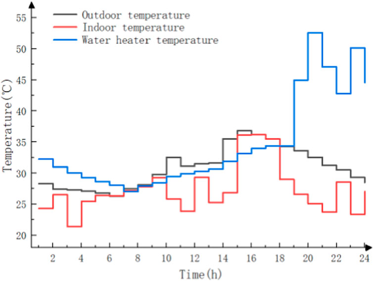
FIGURE 4. Indoor/outdoor temperature and water heater temperature.

FIGURE 5

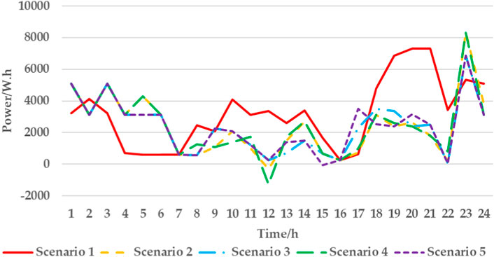
FIGURE 5. Load in different scenarios.

FIGURE 6

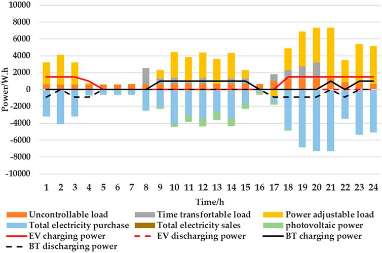
FIGURE 6. Power consumption in Scenario 1.

FIGURE 7

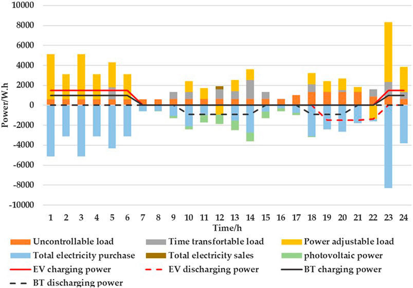
FIGURE 7. Power consumption in Scenario 2.

FIGURE 8

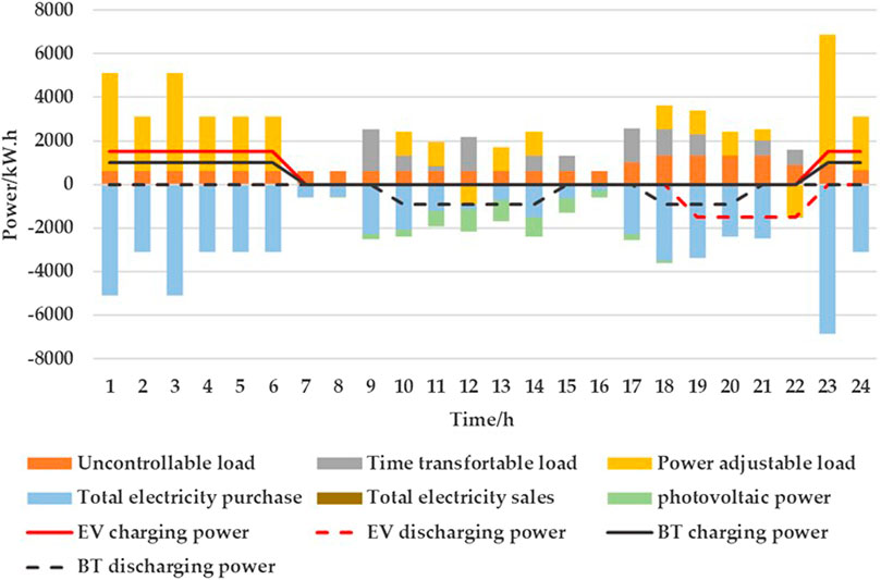
FIGURE 8. Power consumption in Scenario 3.

FIGURE 9

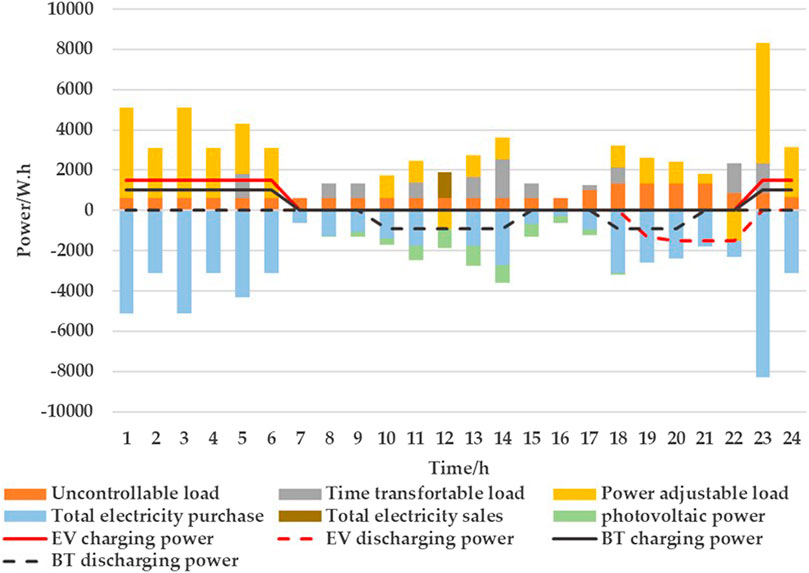
FIGURE 9. Power consumption in Scenario 4.

FIGURE 10

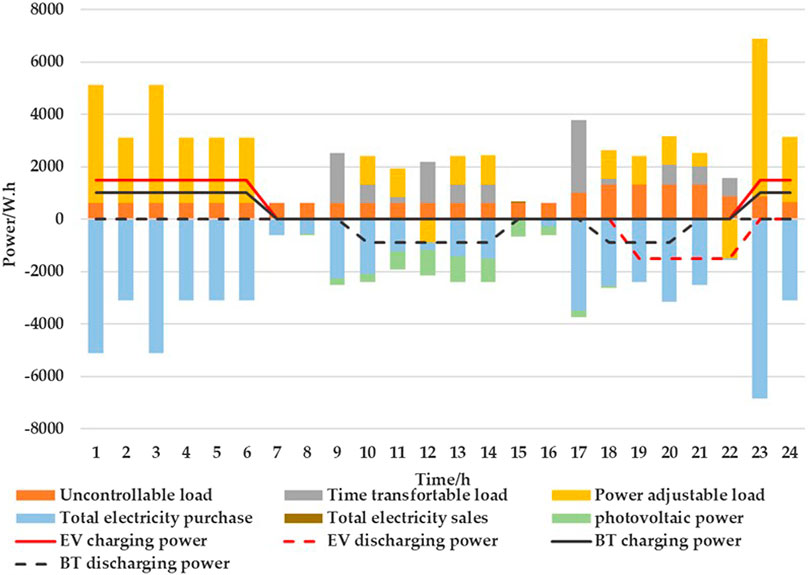
FIGURE 10. Power consumption in Scenario 5.

FIGURE 11

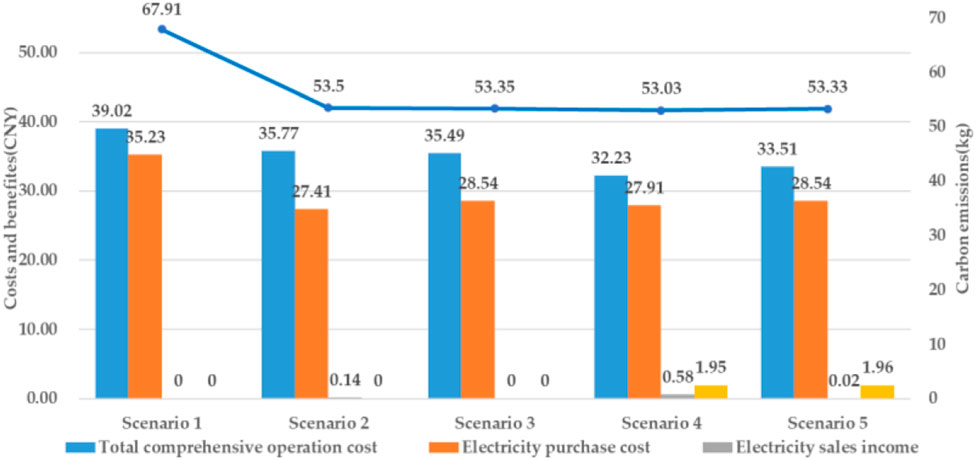
FIGURE 11. Cost and carbon emissions.

TABLE 6

TABLE 6. Battery degradation cost.

6.2 Influence of carbon trading price on dispatching

This paper discusses the influence of carbon trading price on dispatching and adjusts the carbon trading price to 0.39 CNY/kg, 0.49 CNY/kg, 0.59 CNY/kg, and 0.69 CNY/kg, respectively. Table 7 shows the impact of carbon trading prices on the HEMS.

TABLE 7

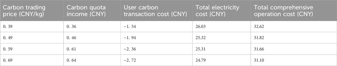
TABLE 7. Impact of carbon trading price on the HEMS.

With the increase in carbon trading price in Table 7, the negative carbon trading cost of users is increasing, the EV carbon quota income is also increasing, and the overall operating cost is decreasing. Therefore, the guidance and regulation of carbon trading prices can play a guiding role in the HEMS.

7 Conclusion

In this paper, the household users’ electricity consumption behavior and carbon quota are considered, and the optimization model of the HEMS which uses price incentives to encourage the users to participate in the carbon interaction is established. A comprehensive total operating cost considering carbon quota and time satisfaction constraints is used to find the solution. The constraints of the user’s load and consumption habits are considered, while considering the cost of battery degradation in both the EV and BT. Then the IPSO algorithm is used to optimize the HEMS, and the effectiveness of IPSO has been demonstrated by a comparison.

Five scenarios were designed based on the optimization model. By the analysis and comparison, it is proved that the comprehensive consideration of carbon trading cost, the battery degradation cost, and total electricity cost can reduce the household carbon emissions and the total electricity cost of the household user better, giving consideration to the user’s electricity habit, operation economy, and battery lifespan. It encourages the end-users to allocate electrical power reasonably. Compared to Scenario 1, the household carbon emissions have been reduced 14.58 kg in Scenario 5, a decrease of over 21.47%, while the total comprehensive operation cost has been reduced by 14.12%. After considering the time satisfaction constraint in Scenario 3, Scenario 5, compared with Scenario 2, Scenario 4, the comprehensive operation cost of the system increases by 1.27 CNY and 1.2 CNY, respectively.

On this basis, the guiding and regulating influences of the carbon trading price on home energy management are analyzed. By the increasing of carbon trading price from 0.39 CNY to 0.69 CNY, the user’s carbon trading income and the EV carbon quota income are increasing from 0.36 CNY to 0.64 CNY, and the overall operating cost is decreasing from 26.03 CNY to 24.79 CNY. The next research direction is to deeply analyze the user’s comfort and load structure utilizing price incentives and carbon trade. Lu and Zhang, 2020.

Data availability statement

The original contributions presented in the study are included in the article/Supplementary material, further inquiries can be directed to the corresponding author.

Author contributions

RY: Writing–original draft, Writing–review and editing. HL: Writing–original draft, Writing–review and editing. CX: Data curation, Formal Analysis, Writing–review and editing. HY: Data curation, Formal Analysis, Methodology, Writing–review and editing. ZY: Data curation, Formal Analysis, Writing–review and editing.

Funding

The author(s) declare financial support was received for the research, authorship, and/or publication of this article. This research was funded by “the science and technology project of the State Grid Corporation of China, Grant Number J2022068.”

Conflict of interest

Authors RY, CX, and HY were employed by State Grid Jiangsu Electric Power Co., LTD.

The remaining authors declare that the research was conducted in the absence of any commercial or financial relationships that could be construed as a potential conflict of interest.

Publisher’s note

All claims expressed in this article are solely those of the authors and do not necessarily represent those of their affiliated organizations, or those of the publisher, the editors and the reviewers. Any product that may be evaluated in this article, or claim that may be made by its manufacturer, is not guaranteed or endorsed by the publisher.

References

Ahmad, A., Khan, A., Javaid, N., Hussain, H. M., Abdul, W., Almogren, A., et al. (2017). An optimized home energy management system with integrated renewable energy and storage resources. Energies 10, 549. doi:10.3390/en10040549

CrossRef Full Text | Google Scholar

Ali, A. O., MohamedElmarghany, R. M., Abdelsalam, M. M., Sabry, M. N., and Hamed, A. M. (2022). Closed-loop home energy management system with renewable energy sources in a smart grid: a comprehensive review. J. Energy Storage 50, 104609. doi:10.1016/j.est.2022.104609

CrossRef Full Text | Google Scholar

Alic, O., and Filik Ü, B. (2021). A multi-objective home energy management system for explicit cost comfort analysis considering appliance category-based discomfort models and demand response programs. Energy Build. 240, 110868. doi:10.1016/j.enbuild.2021.110868

CrossRef Full Text | Google Scholar

Cheng, X., Zheng, Y., Lin, Y., Chen, L., Wang, Y., and Qiu, J. (2021). Hierarchical operation planning based on carbon-constrained locational marginal price for integrated energy system. Int. J. Electr. Power Energy Syst. 128, 106714. doi:10.1016/j.ijepes.2020.106714

CrossRef Full Text | Google Scholar

El Sayed, F., Ghada, M. A., and Hanaa, M. F. (2022). Scheduling home appliances with integration of hybrid energy sources using intelligent algorithms. Ain Shams Eng. J. 13, 101676. doi:10.1016/j.asej.2021.101676

CrossRef Full Text | Google Scholar

Gao, J. W., Gao, F. J., Ma, Z. Y., Huang, N., and Yang, Y. (2021). Multi-objective optimization of smart community integrated energy considering the utility of decision makers based on the Levy flight improved chicken swarm algorithm. Sustain. Cities Soc. 72, 103075. doi:10.1016/j.scs.2021.103075

CrossRef Full Text | Google Scholar

Ikeda., S., and Ryozo, O. (2019). Application of differential evolution-based constrained optimization methods to district energy optimization and comparison with dynamic programming. Appl. Energy 254, 113670. doi:10.1016/j.apenergy.2019.113670

CrossRef Full Text | Google Scholar

Ima, O., Essiet, , Sun, Y. X., and Wang, Z. H. (2019). Optimized energy consumption model for smart home using improved differential evolution algorithm. Energy 172, 354–365. doi:10.1016/j.energy.2019.01.137[

CrossRef Full Text | Google Scholar

Javadi, M. S., Gough, M., Lotfi, M., Esmaeel Nezhad, A., Santos, S. F., and Catalão, J. P. (2020). Optimal self-scheduling of home energy management system in the presence of photovoltaic power generation and batteries. Energy 210, 118568. doi:10.1016/j.energy.2020.118568

CrossRef Full Text | Google Scholar

Khan, Z. A., Zafar, A., Javaid, S., Aslam, S., Rahim, M. H., and Javaid, N. (2019). Hybrid meta heuristic optimization based home energy management system in smart grid. J. Ambient Intell. Humaniz. Comput. 10, 4837–4853. doi:10.1007/s12652-018-01169-y

CrossRef Full Text | Google Scholar

Li, S., Yang, J., Song, W., and Chen, A. (2019). A real-time electricity scheduling for residential home energy management. IEEE Internet Things 6, 2602–2611. doi:10.1109/JIOT.2018.2872463

CrossRef Full Text | Google Scholar

Li, Z. K., and Guo, W. Y. (2020). Optimal operation of integrated energy system considering user interaction. Electr. Power Syst. Res. 187, 106505. doi:10.1016/j.epsr.2020.106505

CrossRef Full Text | Google Scholar

Lu, Q., Guo, Q. S., and Zeng, W. (2021). Optimization scheduling of an integrated energy service system in community under the carbon trading mechanism: a model with reward-penalty and user satisfaction. J. Clean. Prod. 323, 129171. doi:10.1016/j.jclepro.2021.129171

CrossRef Full Text | Google Scholar

Lu, Q., Lü, Sk., Leng, Y. J., and Zhang, Z. (2020). Optimal household energy management based on smart residential energy hub considering uncertain behaviors. Energy 195, 117052. doi:10.1016/j.energy.2020.117052

CrossRef Full Text | Google Scholar

Lu, Q., Zhang, Z., and Lü, S. (2020). Home energy management in smart households: optimal appliance scheduling model with photovoltaic energy storage system. Energy Rep. 6, 2450–2462. doi:10.1016/j.egyr.2020.09.001

CrossRef Full Text | Google Scholar

Merdanoglu, H., Yakıcı, E., Dogan, O. T., Duran, S., and Karatas, M. (2020). Finding optimal schedules in a home energy management system. Electr. Power Syst. Res. 182, 106229. doi:10.1016/j.epsr.2020.106229

CrossRef Full Text | Google Scholar

Nie, Q., Zhang, L., Tong, Z., Dai, G., and Chai, J. (2022). Cost compensation method for PEVs participating in dynamic economic dispatch based on carbon trading mechanism. Energy 239, 121704–121714. doi:10.1016/j.energy.2021.121704

CrossRef Full Text | Google Scholar

Pamulapati, T., Mallipeddi, R., and Lee, M. (2020). Multi-objective home appliance scheduling with implicit and interactive user satisfaction modelling. Appl. Energy 267, 114690. doi:10.1016/j.apenergy.2020.114690

CrossRef Full Text | Google Scholar

Rahima, S., Javaida, N., Ahmada, A., Khan, S. A., Khan, Z. A., Alrajeh, N., et al. (2016). Exploiting heuristic algorithms to efficiently utilize energy management controllers with renewable energy sources. Energy Build. 129, 452–470. doi:10.1016/j.enbuild.2016.08.008

CrossRef Full Text | Google Scholar

Rezaee Jordehi, A. (2019). Enhanced leader particle swarm optimisation (ELPSO): a new algorithm for optimal scheduling of home appliances in demand response programs. Artif. Intell. 53, 2043–2073. doi:10.1007/s10462-019-09726-3

CrossRef Full Text | Google Scholar

Sarker, E., Seyedmahmoudi-an, M., Jamei, E., Horan, B., and Stojcevski, A. (2020). Optimal management of home loads with renewable energy integration and demand response strategy. Energy 210, 118602–118613. doi:10.1016/j.energy.2020.118602

CrossRef Full Text | Google Scholar

Sharififi, A. H., and Maghouli, P. (2019). Energy management of smart homes equipped with energy storage systems considering the PAR index based on real-time pricing. Sustain. Cities Soc. 45, 579–587. doi:10.1016/j.scs.2018.12.019

CrossRef Full Text | Google Scholar

Sun, C., Sun, F., and Moura, S. J. (2016). Nonlinear predictive energy management of residential buildings with photovoltaics & batteries. Power sources. 325, 723–731. doi:10.1016/j.jpowsour.2016.06.076

CrossRef Full Text | Google Scholar

Tan, Q. L., Ding, Y. H., Ye, Q., Mei, S., Zhang, Y., and Wei, Y. (2019). Optimization and evaluation of a dispatch model for an integrated wind photovoltaic-thermal power system based on dynamic carbon emissions trading. Appl. energy 253, 113598. doi:10.1016/j.apenergy.2019.113598

CrossRef Full Text | Google Scholar

Thabo, G., Zhang, J. F., Raj, M. N., Ramesh, C., et al. (2021). Multi-objective economic dispatch with residential demand response programme under renewable obligation. Energy 218, 1–14. doi:10.1016/j.energy.2020.119473

CrossRef Full Text | Google Scholar

Tostado- Véliz., M., Hany, M., Rania, A., Rezaee Jordehi, A., Mansouri, S. A., and Jurado, F. (2023). A fully robust home energy management model considering real time price and on-board vehicle batteries. J. Energy Storage 72, 108531. doi:10.1016/j.est.2023.108531

CrossRef Full Text | Google Scholar

Tostado-Véliz., M., Paul, A., Kamel., S., Zawbaa, H. M., and Jurado, F. (2022). Home energy management system considering effective demand response strategies and uncertainties. Energy Rep. 8, 5256–5271. doi:10.1016/j.egyr.2022.04.006

CrossRef Full Text | Google Scholar

Ubaid ur Rehman., , Kamran, Y., and Khan., M. A. (2022). Optimal power management framework for smart homes using electric vehicles and energy storage. Electr. Power Energy Syst. 134, 107358. doi:10.1016/j.ijepes.2021.107358

CrossRef Full Text | Google Scholar

Wang, S., Guo, D., Han, X., Lu, L., Sun, K., Li, W., et al. (2020a). Impact of battery degradation models on energy management of a grid-connected DC microgrid. Energy 207, 118228. doi:10.1016/j.energy.2020.118228

CrossRef Full Text | Google Scholar

Wang, Y., Qiu, J., Tao, Y., Zhang, X., and Wang, G. (2020b). Low-carbon oriented optimal energy dispatch in coupled natural gas and electricity systems. Appl. Energy 280, 115948. doi:10.1016/j.apenergy.2020.115948

CrossRef Full Text | Google Scholar

Zhu, J., Lin, Y., Lei, W., Liu, Y., and Tao, M. (2019). Optimal household appliances scheduling of multiple smart homes using an improved cooperative algorithm. Energy 171, 944–955. doi:10.1016/j.energy.2019.01.025

CrossRef Full Text | Google Scholar

Zupan cic., J., Filipi c., B., and Gams, M. (2020). Genetic-programming-based multi-objective optimization of strategies for home energy-management systems. Energy 203, 117769. doi:10.1016/j.energy.2020.117769

CrossRef Full Text | Google Scholar