Short-term load forecasting for power systems with high-penetration renewables based on multivariate data slicing transformer neural network

Introduction: The characteristics of intermittency and volatility brought by a high proportion of renewable energy impose higher requirements on load forecasting in modern power system. Currently, load forecasting methods mainly include statistical models and machine learning methods, but they exhibit relative rigidity in handling the uncertainty, volatility, and nonlinear relationships of new energy, making it difficult to adapt to instantaneous load changes and the complex impact of meteorological factors. The Transformer model, as an algorithm used in natural language processing, with its self-attention mechanism and powerful nonlinear modeling capability, can help address the aforementioned issues.

Methods: However, its current performance in time series processing is suboptimal. Therefore, this paper improves the Transformer model through two steps, namely, Data-Slicing and Channel-independence, enhancing its adaptability in load forecasting.

Results: By using load data from Northern Ireland as an example, we compared GRU, CNN, and traditional Transformer models. We validated the effectiveness of this algorithm in short-term load forecasting using MAPE and MSE as indicators.

Discussion: The results indicate that, in short-term load forecasting, the MDS method, compared to GRU, CNN, and traditional Transformer methods, has generally reduced the MSE by over 48%, and achieved a reduction of over 47.6% in MAPE, demonstrating excellent performance.

1 Introduction

The escalation in the integration of renewable energy within the power system stands as a pivotal pathway toward achieving decarbonization (Yang et al., 2022; Østergaard, 2009). Power systems marked by a substantial share of new energy sources are progressively emerging as a forefront issue in the energy sector. In contrast to conventional power systems, those featuring a substantial share of new energy sources often contend with significant fluctuations in instantaneous loads, stemming from the intrinsic instability of these sources (Infield and Freris, 2020). The variability inherent in wind and solar energy can lead to rapid surges or drops in system loads over short periods, thereby placing heightened demands on the stability and dispatchability of the power system. The characteristics of uncertain loads in such systems necessitate the adoption of advanced scheduling and energy storage technologies to effectively mitigate energy fluctuations and ensure the seamless operation of the grid (Wang et al., 2022). Consequently, in power systems characterized by a substantial share of new energy sources, addressing the variability of load characteristics becomes a crucial issue warranting thorough consideration and resolution.

Advanced load forecasting technology emerges as a vital approach in tackling these challenges. The intricacies in this technology predominantly revolve around two key aspects: spatiotemporal complexity and precision. Firstly, owing to the uncertainty and variability of new energy sources, power system load forecasting must adeptly grapple with spatiotemporal complexity (Tascikaraoglu and Sanandaji, 2016). This entails accurately capturing the variations in new energy sources such as wind and solar energy across diverse regions and timeframes, facilitating more nuanced load forecasting for timely and precise adjustments in the face of instantaneous load changes. Secondly, the elevated proportions of new energy source integration necessitate heightened accuracy in load forecasting to ensure the reliability and stability of the power system (Aslam et al., 2021). Precision in load forecasting contributes to the rational planning of generation, storage, and dispatch strategies, thereby enhancing the operational efficiency of the power system and diminishing reliance on conventional backup generation sources. In addition, residential and building loads, especially those related to predicting elastic loads, are also emerging issues this year (Qi et al., 2020; Wan et al., 2021; Qi et al., 2023; Li et al., 2021).

Traditional methods of power system load forecasting predominantly encompass statistical models and machine learning algorithms (Ibrahim et al., 2020). Time series analysis, a common approach among statistical models, relies on historical load data trends and seasonal variations for predictions. Conversely, regression analysis considers various factors influencing load, such as weather and economic activities, and establishes mathematical models for forecasting. While these statistical methods offer simplicity and ease of use, they face limitations in handling intricate nonlinearities and spatiotemporal changes. With the surge of machine learning, an expanding array of algorithms is introduced into the load forecasting domain. Artificial Neural Networks (ANN) represent one such category, simulating complex relationships in load data by mimicking the connections of neurons in the human brain. Moreover, Support Vector Machines (SVM) model nonlinear relationships in data, and ensemble learning methods like decision trees and random forests find application in load forecasting.

However, these methods exhibit shortcomings when confronted with the integration of new energy sources. Firstly, the uncertainty and variability of new energy sources render traditional statistical models relatively inadequate in capturing their spatiotemporal changes (Zhu and Genton, 2012). This results in the inflexibility of traditional time series and regression analyses when addressing instantaneous load changes caused by new energy sources. Secondly, traditional methods face limitations in handling nonlinear relationships, whereas the characteristics of new energy sources often involve intricate nonlinear relationships, such as the nonlinear connection between photovoltaic power generation and solar radiation. This may lead to a performance decline of traditional algorithms in adapting to the complex scenarios of integrating new energy sources into the power system. The main root of this problem lies in the characteristics and assumptions of the models themselves. Traditional statistical models like linear regression are built on the assumption of linearity, while complex relationships in the real world are often nonlinear, making it challenging for these models to accurately capture them. Machine learning algorithms may face issues of overfitting or underfitting, and the curse of dimensionality leads to a decline in the generalization performance of models on high-dimensional data. Factors such as parameterization constraints, lack of flexibility, and reliance on large-scale annotated data also contribute to the inadequacies. Additionally, the seasonal and meteorological factors of new energy sources impact load forecasting, and traditional methods may lack the flexibility required for modeling these factors. Therefore, when confronting the challenges of integrating new energy sources into power systems, more advanced and flexible load forecasting methods are essential, such as algorithms based on deep learning.

The Transformer model, initially designed for natural language processing, has exhibited exceptional performance in addressing these challenges (Lauriola et al., 2022). Firstly, the Transformer model excels in capturing spatiotemporal relationships by modeling global correlations in sequence data through self-attention mechanisms. This capability allows it to flexibly adapt to the intricate spatiotemporal characteristics of new energy load fluctuations, effectively managing their uncertainty and instantaneous changes compared to traditional statistical models and machine learning algorithms. Secondly, the Transformer model possesses robust nonlinear modeling capabilities (Martinez and Mork, 2005). Given that the characteristics of integrating new energy sources into power systems may involve complex nonlinear relationships, the Transformer can capture intricate dependencies between different features through multi-head self-attention mechanisms, better accommodating the nonlinear changes in load. Furthermore, the Transformer model performs well in addressing long-term dependency issues, critical for factors such as seasonality and meteorological influences in load forecasting. Through self-attention mechanisms, the Transformer can effectively capture dependencies between different time steps in time series data, contributing to more accurate predictions of load changes at various time scales (Rao et al., 2021).

However, recent studies have indicated that a very simple linear model outperforms all previous Transformer-based models in a series of common benchmark tests, casting doubt on the practicality of Transformers in time series forecasting. These challenges include high spatiotemporal complexity and insufficient learning ability for long look-back windows, hindering the further advancement of Transformer models in power system load forecasting.

Therefore, this paper introduces the Multivariate Data Slicing Transformer (MDS-Transformer) Model to optimize the performance of the Transformer model in load point forecasting, addressing these challenges. This model incorporates two key designs: Data-Slicing and Channel-independence. Firstly, recognizing that the goal of time series forecasting is to comprehend data correlations between different time steps, the model aggregates time steps into slices at the sub-series level to extract local semantic information, enhancing locality and capturing comprehensive semantic information not available at the point level. Secondly, in the context of multivariate time series as a multi-channel signal, each Transformer input token can be represented by data from a single channel or multiple channels. The Channel-independence design ensures that each input token contains information from a single channel only, differing from previous methods applied to CNN and linear models.

2 The framework of multivariate data slicing transformer model

2.1 Fundamental components of transformer model

The Transformer model is a type of deep learning model originally proposed by Vaswani in 2017 (Rao et al., 2021) for sequence-to-sequence tasks. The overview of Transformer model can be seen in Figure 1. It introduces a self-attention mechanism, allowing the model to simultaneously attend to different positions in the input sequence without the need for sequential processing. The main components of the Transformer model include:

1) Input Representation: The input sequence undergoes an initial phase where it traverses through an embedding layer. In this layer, each word or token within the sequence is meticulously mapped to a vector representation within a high-dimensional space. This representation is commonly referred to as input embedding, expressed by formula (1) as:

$InputEmbedding:X=\left[x_1,x_2,\dots ,x_n\right](1)$

Where $X=\left[x_1,x_2,\dots ,x_n\right]$ is the input sequence, $n$ is the sequence length, and $x_i$ is a word or token.

2) Positional Encoding: Given that the Transformer inherently lacks explicit sequential information, a crucial step involves incorporating positional encoding into the input embeddings. This addition serves the purpose of introducing the sequential order of the sequence. Consequently, the model becomes adept at distinguishing between words positioned at various points within the sequence. This relationship is represented by Eqs 3, 4:

$P{E}_{\left(pos,2i\right)}=\sin \left(\frac{pos}{{10000}^{2i/{\mathrm{d}}_{\text{model}}}}\right)(2)$

$P{E}_{\left(pos,2i+1\right)}=\cos \left(\frac{pos}{{10000}^{2i/d_{\text{model}}}}\right)(3)$

Where $pos$ is the position, $i$ is the index of the dimension, and $d_{\text{model}}$ is the dimension of embedding.

3) Encoder: The encoder is structured with multiple identical layers, each encompassing two sub-layers:

i. Self-Attention Layer: This layer operates by computing attention weights, ensures the model to allocate distinct attention to each position within the sequence (He et al., 2022), which facilitates the model to selectively focus on different positions of information during the processing of input sequence:

$\text{Attention}\left(Q,K,V\right)=\text{softmax}\left(\frac{Q{K}^T}{\sqrt{d_k}}\right)V(4)$

In (Eq. 4), $\text{Attention}$ represents the self-attention computation results. $Q$ stands for the query matrix, used to calculate attention weights. $K$ represents the key matrix, also used to calculate attention weights. $V$ represents the value matrix, which is a matrix obtained by weighting according to attention weights.

$\text{FFN}\left(x\right)=\max \left(0,x{W}_1+b_1\right)W_2+b_2(5)$

In (Eq. 5), $x$ represents the output of the self-attention layer, and $W_b$, $b_1$, $W_2$, $b_2$ represent the weights and biases of the feedforward neural network. FFN represents the output of the feedforward neural network.

4) Multi-Head Attention Mechanism: By employing multiple attention heads, the model can learn different attention weights and then concatenate them together. Multiple attention heads can be represented by formulas (6) and (7):

$\text{MultiHead}\left(Q,K,V\right)=\text{Concat}\left({\text{head}}_1,\dots ,{\text{head}}_h\right)W_O(6)$

${\text{head}}_i=\text{Attention}\left(Q{W}_{Q_i},K{W}_{K_i},V{W}_{V_i}\right)(7)$

In (Eq. 7), $\text{MultiHead}$ represents the output of the multi-head attention mechanism, and ${\text{head}}_i$ represents the output of the $i$-th attention head. $W$ denotes the weights for the linear transformations in the multi-head attention mechanism.

5) Residual Connection and Layer Normalization: Following each sub-layer is a residual connection and layer normalization, which helps prevent the vanishing or exploding gradients during the training process.

6) Stacked Encoder Layers: The entire encoder is constructed by stacking multiple identical layers together.

i. Decoder: The decoder mirrors the encoder’s architecture and comprises multiple identical layers. Each decoder layer consists of three sub-layers:

ii. Self-Attention Layer: Resembling the self-attention layer in the encoder, the decoder’s self-attention layer operates with the distinction that each position can exclusively attend to its own preceding positions.

iii. Feedforward Neural Network: This sub-layer mirrors the feedforward neural network in the encoder.

iv. Final Output Layer: The output generated by the decoder undergoes a linear transformation followed by a softmax operation. The output expression can be represented by Eq. 8.

$\text{Output}\left(x\right)=\text{softmax}\left(x{W}_O+b_O\right)(8)$

FIGURE 1

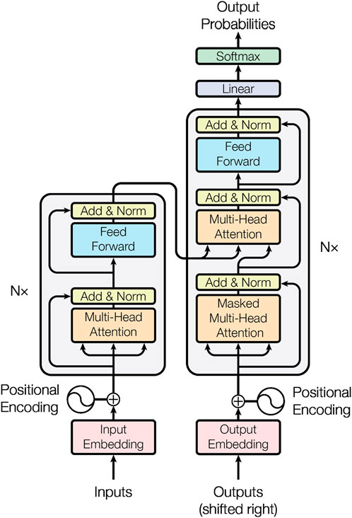
FIGURE 1. The overview of Transformer model.

ii. Feedforward Neural Network: Following each attention layer is a fully connected feedforward neural network. This network is position-wise independent (Bouktif et al., 2018):

Where Output represents the probability distribution of the final output.

2.2 MDS approach

In the context of load forecasting, we consider the following issues: given a set of multivariate load sequence samples, where each time step $x_t$ is a vector of dimension M, we aim to predict the load values for the next T time steps $\left(xL+1;...;xL+T\right)$ using data from a past time window $L:\left(x1;...;xL\right)$. This is a typical load forecasting problem, crucial for the management of power systems and energy planning. To address this challenge, we introduce a model called Multivariate Data Slicing (MDS), as shown in Figure 2. The architecture of MDS is based on a vanilla Transformer encoder, which is a deep learning model initially used in natural language processing but has been successfully applied in various fields. In the context of our load forecasting, the core objective of MDS is to enhance predictive performance for load variations by aggregating local information from the load data.

1) Forward Process: In the forward process, we define the $i$-th univariate time series of length $x_{1:L}^{\left(i\right)}=\left(x_i^{\left(1\right)},\dots ,x_i^{\left(L\right)}\right)$, where $i=1,\dots ,M$. The input data $x_{1:L}=\left(x_1,\dots ,x_L\right)$ is divided into $M$ univariate time series $x^{\left(i\right)}\in {\mathbb{R}}^{1\times L}$, where each sequence is a vector of dimension $1\times L$. This segmentation is designed to adhere to channel independence.

FIGURE 2

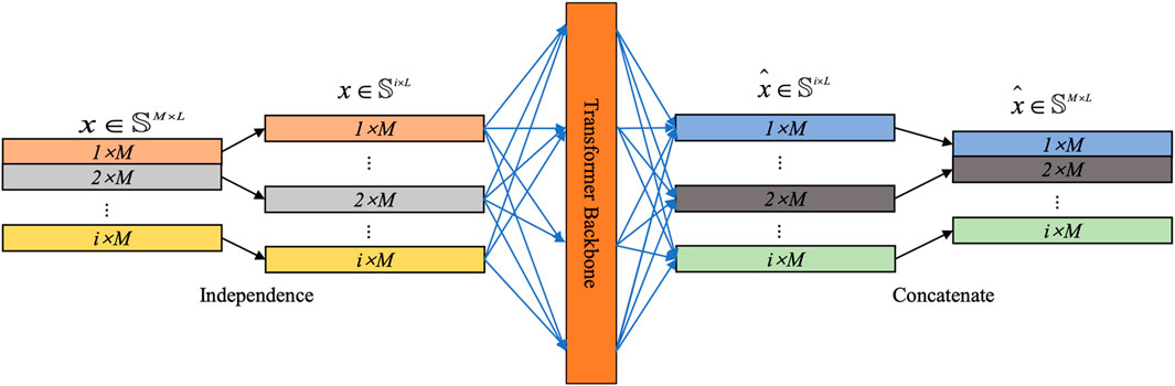
FIGURE 2. The overview of MDS-Transformer model.

Subsequently, these segmented univariate time series $x^{\left(i\right)}$ are independently fed into the backbone structure of the Transformer. The Transformer is a deep learning model renowned for its powerful performance in sequence modeling tasks. Under the processing of the Transformer, the backbone structure provides prediction results $x^{\prime \left(i\right)}=\left({\widehat{x}}^{\left(Li+1\right)},\dots ,{\widehat{x}}^{\left(Li+T\right)}\right)$ in ${\mathbb{R}}^{1\times T}$ for each univariate time series $x^{\left(i\right)}$. This signifies the predicted values for the next $T$ time steps, where ${\widehat{x}}^{\left(Li+1\right)},\dots ,{\widehat{x}}^{\left(Li+T\right)}$ represent the predicted values from time step $Li+1$ to $Li+T$.

2) Data Slicing: The introduction of patching can significantly enhance the comprehension of electricity load data. Traditional load forecasting methods often rely on single time-step information or manually extracted features. However, these approaches face limitations as they struggle to adequately capture the intricate relationships and local patterns inherent in electricity load data.

By implementing Data Slicing, which involves aggregating time steps into “Slices” at the subsequence level, the model gains the ability to more effectively capture local features in the variations of electricity load. Each “Slice” can represent a segment of load data over a specific period, providing a more comprehensive reflection of local patterns and changes within the system. This methodology enables a more nuanced understanding of the complex dynamics inherent in electricity load data.

The process of the “Slicing” method is as follows. For each input univariate time series $x^{\left(i\right)}$, it is initially segmented into patches, which can be overlapping or non-overlapping. The length of the patches is denoted as $P$, and the stride is denoted as $S$, where the stride represents the non-overlapping region between two adjacent patches. Therefore, the patching process generates a patch sequence $x^{\left(p_i\right)}\in {\mathbb{R}}^{P\times N}$, where $N$ is the number of patches, $N=\lfloor \left(L-SP\right)/P\rfloor +2$. Prior to Slicing, the end of the original sequence needs to be padded with $S$ repetitions of the last value $x^{\left(L\right)}$.

By using patching, the number of input tokens can be reduced from $L$ to approximately $L/S$. This means that the memory usage and computational complexity of attention maps both decrease quadratically by a factor of $S$. Therefore, within the constraints of training time and GPU memory, patch design allows the model to see longer historical sequences. By reducing the number of input tokens, this slicing method provides the model with the ability to handle longer historical sequences, potentially yielding more accurate results in tasks such as load forecasting.

3) Transformer Encoder: In this model, a basic Transformer encoder is utilized to map the observed signals to latent representations. Mapping is performed on these patches through a trainable linear projection matrix $W_p\in {\mathbb{R}}^{D\times P}$ and a learnable positional encoding matrix $W_{\text{pos}}\in {\mathbb{R}}^{D\times N}$, used to capture the temporal sequence of the patches. Here, $D$ is the dimension of the Transformer’s latent space, and $N$ is the number of patches. Specifically, the patch $x^{\left(di\right)}\in {\mathbb{R}}^{D\times N}$ is given by the formula: $x^{\left(di\right)}=W_p{x}^{\left(pi\right)}+W_{\text{pos}}$, where $x^{\left(pi\right)}$ is the patch subjected to linear projection and positional encoding.

Next, each head $h=1,\dots ,H$ in the multi-head attention transforms these inputs into query matrices $Q^{\left(hi\right)}={\left(x^{\left(di\right)}\right)}^T{W}_{hQ}$, key matrices $K^{\left(hi\right)}={\left(x^{\left(di\right)}\right)}^T{W}_{hK}$, and value matrices $V_h^{\left(i\right)}={\left(x^{\left(di\right)}\right)}^T{W}_{hV}$, where $W_{hQ},W_{hK}\in {\mathbb{R}}^{D\times d_k}$ and $W_{hV}\in {\mathbb{R}}^{D\times D}$. Subsequently, the scaled dot-product operation produces attention outputs $O^{\left(hi\right)}\in {\mathbb{R}}^{D\times N}$: ${\left(O^{\left(hi\right)}\right)}^T=\text{Attention}\left(Q^{\left(hi\right)},K^{\left(hi\right)},V_h^{\left(i\right)}\right)=\text{Softmax}\left(Q^{\left(hi\right)}{K}^{\left(hi\right)}/\sqrt{d_k}\right)V_h^{\left(i\right)}$. The multi-head attention block also includes a batch normalization layer and a feedforward network with residual connections. Following this, it generates representations $z^{\left(i\right)}\in {\mathbb{R}}^{D\times N}$.

Finally, a flattening layer with linear heads is used to obtain prediction results $x^{\prime \left(i\right)}=\left({\widehat{x}}^{\left(Li+1\right)},\dots ,{\widehat{x}}^{\left(Li+T\right)}\right)\in {\mathbb{R}}^{1\times T}$. These operations describe the structure of the attention mechanism, multi-head attention block, and feedforward network in the MDS model, and how these components are integrated to obtain predictions for future time steps.

4) Loss Function: We choose to use Mean Squared Error (MSE) loss to measure the difference between predicted values and actual values (Han et al., 2021). The loss is computed on each channel, and then averaged across M time series to obtain the overall objective loss:

$L=\frac{1}{M}{\displaystyle \sum _{i=1}^M}\frac{1}{T}{\displaystyle \sum _{t=1}^T}{‖{\widehat{x}}^{\left(Li+t\right)}-x^{\left(Li+t\right)}‖}_2^2(9)$

In this formula (9), ${\widehat{x}}^{\left(Li+t\right)}$ represents the model’s predicted value for the $i$-th time series at time step $Li+t$, and $x^{\left(Li+t\right)}$ represents the actual observed value (Bo et al., 2023). Mean Squared Error calculates the difference between predicted and actual values at each time step and obtains the overall loss by summing the squares and taking the average. This overall loss $L$ reflects the model’s predictive performance across all time series and time steps. During the training process, the goal of the optimization algorithm is typically to minimize this Mean Squared Error loss, aiming to improve the model’s accuracy in predicting future time steps (Sampath et al., 2021).

5) Instance Normalization: This technique, recently proposed, aims to help alleviate the distribution shift effects between training and testing data. It straightforwardly standardizes each time series instance $x^{\left(i\right)}$, giving it a zero mean and unit standard deviation (Ahmadi et al., 2016). Essentially, we normalize each $x^{\left(i\right)}$ before slicing, and then add back the mean and standard deviation to the output predictions.

2.3 Representation learning

Self-supervised representation learning is widely utilized to derive high-level abstract representations from unlabeled data. In this section, we leverage the MDS method to obtain effective representations for multivariate time series, showcasing their successful applicability in prediction tasks. Masked autoencoders, a well-established technique in natural language processing (NLP) and computer vision (CV) domains, constitute one of the popular methods for self-supervised pretraining of learned representations (Vaswani et al., 2017).

The fundamental concept behind masked autoencoders is straightforward: deliberately omit a random segment of the input sequence and train the model to reconstruct the missing content (Ericsson et al., 2022). Recent advancements have introduced masked encoders to the time series domain, demonstrating their efficacy in classification and regression tasks. Integrating multivariate time series into the Transformer framework involves representing each input token as a vector containing the time series values at a specific time step (George et al., 2021). Masks are randomly positioned within each time series and across different sequences.

However, this configuration presents two potential challenges. Firstly, masks are applied at the individual time step level. The values for the current time step’s mask can be easily deduced by interpolating with its adjacent time values, lacking the necessity for a holistic understanding of the entire sequence. This contradicts the overarching objective of learning crucial abstract representations for the entire signal. To address this issue, intricate randomization strategies have been proposed, involving the random masking of differently sized time series.

Secondly, designing an output layer for prediction tasks may face some challenges (Kahng et al., 2017). Given representation vectors $z_t\in {\mathbb{R}}^D$ corresponding to all $L$ time steps, mapping these vectors to outputs containing $M$ variables, each with a prediction range of $T$, requires a parameter matrix $W$ with dimensions $\left(L\cdot D\right)\times \left(M\cdot T\right)$. If one or more of these four values are large, this matrix may become exceptionally large. This could lead to overfitting, especially when downstream training samples are scarce.

The proposed MDS method naturally overcomes the above issues. We use the same Transformer encoder as in a supervised setting, but remove the prediction head and add a linear layer of $D\times P$. Unlike in supervised models where overlapping patches are allowed, we divide each input sequence into regular non-overlapping patches. This design ensures that observed patches do not contain information about the masked patches. Next, we uniformly and randomly select a subset of patch indices and mask the patches with zero values based on these selected indices. The model is trained using Mean Absolute Percentage Error loss to reconstruct the masked patches.

It is worth emphasizing that each time series will have its own latent representation, learned through weight sharing across tasks. This design allows pretraining data to include more time series than downstream data, which is challenging for other methods to achieve.

3 Case study

To validate the aforementioned approach, we focused our study on the Irish energy system and conducted short-term load forecasting. The European Union target for the Irish energy system stipulates that 16% of the country’s total energy consumption should come from renewable sources by 2020. Energy in Ireland is predominantly utilized for heating, transportation, and electricity. To meet the 16% energy target, EirGrid, the transmission system operator, aims to have 40% of the electricity sourced from renewable resources on the island of Ireland by 2020. The overarching goal of the DS3 (Delivering a Secure, Sustainable Electricity System) program is to augment the share of renewable energy in the Irish electricity system in a secure and reliable manner, ultimately fulfilling Ireland’s 2020 electricity target.

3.1 Data description

Our dataset spans approximately 6.5 years, from 1 January 2014, 00:00, to 30 April 2020, 23:45, and originates from the Irish energy system. It encompasses various aspects of electricity data, including power generation, power demand, wind power generation, and other indicators, covering both Ireland and Northern Ireland. The dataset comprises unprocessed 15-min original SCADA readings, with the unit of load data measured in megawatts (MW) and updates occurring every 15 min. Notably, the dataset boasts high completeness and proves to be well-suited for research endeavors related to short-term load forecasting and distribution optimization in power systems.

The data is sourced from the EirGrid Group, serving as the Transmission System Operator (TSO) in Ireland. EirGrid, a state-owned company, is tasked with managing and operating the entire transmission network on the island of Ireland. Its high-voltage network receives power from generators and supplies wholesale energy to a substantial number of users. Furthermore, EirGrid plays a crucial role in providing distribution networks, forecasting when and where electricity is needed in both Ireland and Northern Ireland. These predictions span various timeframes, including hourly, daily, and annually.

3.2 Result analysis

In our evaluation, we use Mean Absolute Percentage Error (MAPE) and Mean Square Error (MSE) and training time as key metrics. MAPE is a widely used metric for measuring prediction errors, particularly applied to assess the accuracy of time series data or other forecasting models. The outcomes of MAPE are presented as percentages, representing the average percentage error of each forecasted value relative to the actual value. A lower MAPE value signifies greater accuracy in the model’s predictions. The expressions for MAPE and MSE can be represented by Eqs 10, 11:

$MAPE=\frac{1}{n}{\sum }_{i=1}^n\left|\frac{y_i-\stackrel{\mu }{y_i}}{y_i}\right|\times 100\%(10)$

$MSE=\frac{1}{n}{{\sum }_{i=1}^n\left|y_i-\stackrel{\mu }{y_i}\right|}^2(11)$

By default, this method consists of three encoder layers, with a head count (H) of 16 and a latent space dimension (D) of 128. The feedforward network in the Transformer encoder block is composed of two linear layers with GELU activation function: one layer projects the hidden representation (D = 128) into a new dimension (F = 256), and the other layer projects it back to D = 128. For very small datasets, reducing the size of parameters (H = 4, D = 16, and F = 128) is recommended to alleviate potential overfitting. In all experiments, a dropout with a probability of 0.2 is applied in the encoder. In addition, the hyperparameters used during the MDS method training process are shown in Table 1:

TABLE 1

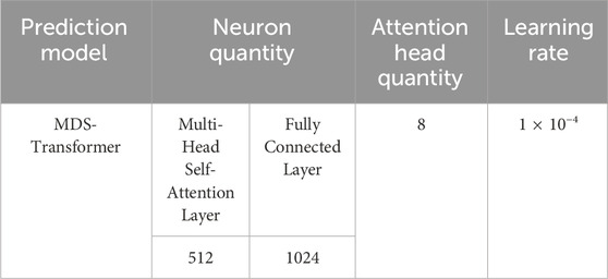
TABLE 1. Model hyperparameter Configuration.

Utilizing the MDS-Transformer model, we conducted joint predictions as well as separate load predictions for NI Demand, NI Wind Generation, and NI Wind Availability. This approach was undertaken to validate the potential advantages of multivariate joint forecasting. The corresponding data results are presented in Table 2:

TABLE 2

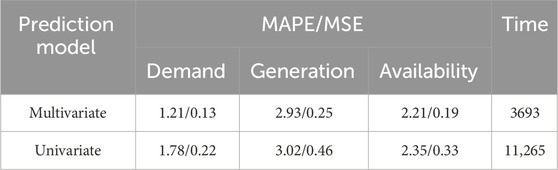
TABLE 2. Predicting NI Demand, NI Wind Generation, and NI Wind Availability using two types of forecasting models: multivariate and univariate.

From Table 2, it is evident that the error associated with the multivariate load joint forecasting method is slightly smaller than that of individual load forecasting. Moreover, the training time is notably reduced by 67.2%, a significant improvement compared to individual load forecasting. This reduction in training time can be attributed to the fact that individual load forecasting necessitates modeling and solving for different types of loads separately, whereas multivariate load joint forecasting can output multivariate load data simultaneously, thereby substantially enhancing computational efficiency. The analysis of the inherent connections between multivariate loads also contributes to an improvement in prediction accuracy to a certain extent. This reaffirms the efficiency and effectiveness of the multivariate load joint forecasting approach. In the subsequent comparative analysis section, all models will adopt the multivariate load joint forecasting method.

To validate the superiority of the MDS-Transformer in the multivariate short-term load forecasting problem, this study conducts a comparative analysis with well-established GRU and CNN models commonly used in the field of time series forecasting. Simultaneously, to assess the effectiveness of the proposed improvement, the predictive results of the traditional Transformer model are compared with those of the MDS-Transformer model. The obtained predictions for each model are illustrated in Figures 3–5 for a 48-h forecast and Figures 6–8 for a 168-h forecast. Evaluation data on NI demand is presented in Table 3.

FIGURE 3

FIGURE 3. Utilizing four different methods to conduct a 48-h forecast for NI Demand.

FIGURE 4

FIGURE 4. Utilizing four different methods to conduct a 48-h forecast for NI Wind Generation.

FIGURE 5

FIGURE 5. Utilizing four different methods to conduct a 48-h forecast for NI Wind Availability.

FIGURE 6

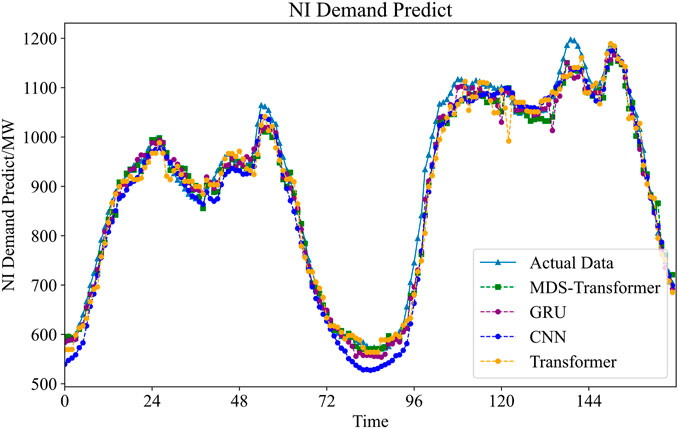
FIGURE 6. Utilizing four different methods to conduct a 168-h forecast for NI Demand.

FIGURE 7

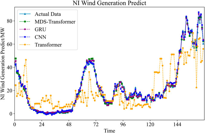
FIGURE 7. Utilizing four different methods to conduct a 168-h forecast for NI Wind Generation.

FIGURE 8

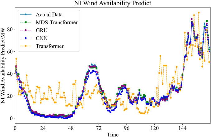
FIGURE 8. Utilizing four different methods to conduct a 168-h forecast for NI Wind Availability.

TABLE 3

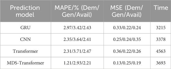
TABLE 3. Predicting result of NI Demand, NI Wind Generation, and NI Wind Availability using 4 types of forecasting models: GRU, CNN, Transformer and MDS-Transformer.

From the results, it can be observed that, relying on the multi-scale attention mechanism to capture spatiotemporal dependencies at different scales, as well as the improved data slicing function, the MDS-Transformer exhibits the highest prediction accuracy, closely aligning with the actual data throughout the entire time period. Although GRU and Transformer also demonstrate strong predictive capabilities, they slightly lag behind MDS-Transformer, particularly exhibiting slight deviations near peaks and troughs. In contrast, the CNN shows relatively lower fitting accuracy, with significant deviations near peaks and troughs.

The MDS method demonstrates outstanding performance in multiple aspects. Whether in terms of MAPE or MSE, the results of the MDS method are superior. This superiority is most pronounced in load forecasting, where MAPE decreases by nearly 50%, and MSE decreases by almost 60%. As the MDS method aggregates time steps into slices and processes them at the subsequence level, it can better understand the data correlations between different time steps. For load forecasting, this means that the model is more capable of capturing short-term variations and trends in load data, leading to more accurate predictions.

In the case of wind power forecasting, MDS achieves a 14.2% reduction in MAPE compared to the GRU method, with the most significant improvement being a 21.0% increase compared to the transformer model. However, this improvement is not as substantial as in load forecasting, possibly because wind power forecasting involves more long-term trends and seasonal variations. The MDS Transformer is designed to emphasize understanding the local data correlations within short-term intervals, which might explain the relatively smaller improvement in the context of wind power forecasting.

From the statistical results, it is evident that the MDS-Transformer model, incorporating Data Slicing and Channel-independence, exhibits a significant improvement in predictive performance for NI demand compared to traditional GRU and CNN models. This improvement can be attributed to the incomplete penetration of wind power, with NI wind generation and NI Wind Availability remaining lower than NI demand. The model strategically focuses its attention on the larger magnitude of NI demand, thereby enhancing overall predictive accuracy.

In comparison to the traditional Transformer model, the Mean Absolute Percentage Error (MAPE) for NI demand, NI Wind Generation, and NI Wind Availability decreases by 47.62%, 21.02%, and 10.53%, respectively, indicating a notable enhancement in overall predictive accuracy. Despite the MDS-Transformer having a more complex network structure and longer training times for each iteration, improvements in the attention mechanism and gate residual links at both the self-attention and network structure levels significantly boost training efficiency. This enables the model to reach optimal values more quickly, reducing the overall training duration. Compared to the traditional Transformer model, the training time is reduced by 19.07%, striking a balance between learning efficiency and predictive performance, within an acceptable range.

4 Conclusion

This paper addresses the short-term forecasting problem of multivariate loads in renewable energy systems and introduces a predictive method based on the MDS-Transformer model. The model extracts high-dimensional data features through Data Slicing, utilizes a multi-head self-attention mechanism to capture key information from input features, and stabilizes the network structure through gate-controlled residuals. The following conclusions are drawn from the case analysis:

1) The joint forecasting approach for multivariate loads outperforms single-variable load forecasting in the short-term prediction of multivariate loads. This approach significantly improves computational efficiency while ensuring predictive accuracy.

2) The self-attention mechanism effectively leverages the predictive capabilities of the Transformer model by analyzing the coupling relationships of multivariate loads. It achieves higher predictive accuracy compared to traditional time series forecasting models but comes with a relatively slower computational speed.

3) Both the multi-head self-attention mechanism and the gate-controlled residual method enhance the predictive capabilities of the Transformer model to varying degrees in the short-term forecasting of multivariate loads. Their combined effects significantly improve the model’s predictive accuracy, training efficiency, and forecasting stability.

This method is a short-term prediction approach based on point forecasting. The predicted results can provide specific values for real-time scheduling in power plants, ensuring the safe and stable operation of the power grid, as well as peak shaving in grid operations to enhance overall efficiency. However, if applied to demand-side response, which involves incentivizing users to adjust their electricity consumption behavior to balance the supply and demand of the grid, this method may still have limitations. In such cases, the use of probability forecasting is necessary. Probability forecasting can provide the likelihood of the load falling within a certain range, facilitating the formulation of strategies for demand-side response and improving its effectiveness.

Data availability statement

The original contributions presented in the study are included in the article/supplementary material, further inquiries can be directed to the corresponding author.

Author contributions

WL: Writing–original draft. XC: Writing–review and editing.

Funding

The author(s) declare financial support was received for the research, authorship, and/or publication of this article. This study received funding from the Research Project on Science and Technology of Chongqing Education Committee in 2019 (KJQN201905803). The funder was not involved in the study design, collection, analysis, interpretation of data, the writing of this article or the decision to submit it for publication.

Conflict of interest

The authors declare that the research was conducted in the absence of any commercial or financial relationships that could be construed as a potential conflict of interest.

Publisher’s note

All claims expressed in this article are solely those of the authors and do not necessarily represent those of their affiliated organizations, or those of the publisher, the editors and the reviewers. Any product that may be evaluated in this article, or claim that may be made by its manufacturer, is not guaranteed or endorsed by the publisher.

References

Ahmadi, M., Ulyanov, D., Semenov, S., Trofimov, M., and Giacinto, G. (2016). “Novel feature extraction, selection and fusion for effective malware family classification,” in Proceedings of the sixth ACM conference on data and application security and privacy, New Orleans Louisiana USA, 11 March 2016, 183–194.

CrossRef Full Text | Google Scholar

Aslam, S., Herodotou, H., Mohsin, S. M., Javaid, N., and Ashraf, N. (2021). A survey on deep learning methods for power load and renewable energy forecasting in smart microgrids. Renew. Sustain. Energy Rev. 144, 110992. doi:10.1016/j.rser.2021.110992

CrossRef Full Text | Google Scholar

Bo, X., Chenggong, Q., Junwei, N., Songyun, W., Guoqiang, S., and Yizhou, Z. (2023). Cluster analysis of minute load data based on deep autoencoder. Guangdong Electr. Power 36 (3), 57–67. doi:10.3969/i.issn.1007-290X.2023.03.007

CrossRef Full Text | Google Scholar

Bouktif, S., Fiaz, A., Ouni, A., and Serhani, M. (2018). Optimal deep learning lstm model for electric load forecasting using feature selection and genetic algorithm: comparison with machine learning approaches. Energies 11 (7), 1636. doi:10.3390/en11071636

CrossRef Full Text | Google Scholar

Ericsson, L., Gouk, H., Loy, C. C., and Hospedales, T. M. (2022). Self-supervised representation learning: introduction, advances, and challenges. IEEE Signal Process. Mag. 39 (3), 42–62. doi:10.1109/msp.2021.3134634

CrossRef Full Text | Google Scholar

George, Z., Jayaraman, S., Patel, D., Bhamidipaty, A., and Eickhoff, C. (2021). A transformer-based framework for multivariate time series representation learning. In Proceedings of the 27th ACM SIGKDD Conference on Knowledge Discovery and Data Mining, Singapore, August 14 - 18, 2021, 2114–2124.

Google Scholar

Han, K., Xiao, A., Wu, E., Guo, J., Xu, C., and Wang, Y. (2021). Transformer in transformer. Adv. Neural Inf. Process. Syst. 34, 15908–15919. doi:10.48550/arXiv.2103.00112

CrossRef Full Text | Google Scholar

He, K., Chen, X., Xie, S., Li, Y., Dollár, P., and Girshick, R. (2022). “Masked autoencoders are scalable vision learners,” in Proceedings of the IEEE/CVF conference on computer vision and pattern recognition, New Orleans, LA, USA, June 18 2022 to June 24 2022, 16000–16009.

CrossRef Full Text | Google Scholar

Ibrahim, M. S., Dong, W., and Yang, Q. (2020). Machine learning driven smart electric power systems: current trends and new perspectives. Appl. Energy 272, 115237. doi:10.1016/j.apenergy.2020.115237

CrossRef Full Text | Google Scholar

Infield, D., and Freris, L. (2020). Renewable energy in power systems. New Jersey, United States: John Wiley and Sons.

Google Scholar

Kahng, M., Andrews, P. Y., Kalro, A., and Chau, D. H. (2017). A cti v is: visual exploration of industry-scale deep neural network models. IEEE Trans. Vis. Comput. Graph. 24 (1), 88–97. doi:10.1109/tvcg.2017.2744718

PubMed Abstract | CrossRef Full Text | Google Scholar

Lauriola, I., Lavelli, A., and Aiolli, F. (2022). An introduction to deep learning in natural language processing: models, techniques, and tools. Neurocomputing 470, 443–456. doi:10.1016/j.neucom.2021.05.103

CrossRef Full Text | Google Scholar

Li, Z., Wu, L., Xu, Y., and Zheng, X. (2021). Stochastic-weighted robust optimization based bilayer operation of a multi-energy building microgrid considering practical thermal loads and battery degradation. IEEE Trans. Sustain. Energ. 13 (2), 668–682. doi:10.1109/TSTE.2021.3126776

CrossRef Full Text | Google Scholar

Martinez, J. A., and Mork, B. A. (2005). Transformer modeling for low-and mid-frequency transients-a review. IEEE Trans. Power Deliv. 20 (2), 1625–1632. doi:10.1109/tpwrd.2004.833884

CrossRef Full Text | Google Scholar

Østergaard, P. A. (2009). Reviewing optimisation criteria for energy systems analyses of renewable energy integration. Energy 34 (9), 1236–1245. doi:10.1016/j.energy.2009.05.004

CrossRef Full Text | Google Scholar

Qi, N., Cheng, L., Xu, H., Wu, K., Li, X., Wang, Y., et al. (2020). Smart meter data-driven evaluation of operational demand response potential of residential air conditioning loads. Appl. Energy 279, 115708. doi:10.1016/j.apenergy.2020.115708

CrossRef Full Text | Google Scholar

Qi, N., Pinson, P., Almassalkhi, M. R., Cheng, L., and Zhuang, Y. (2023). Chance-Constrained generic energy storage operations under decision-dependent uncertainty. IEEE Trans. Sustain. Energy 14, 2234–2248. doi:10.1109/tste.2023.3262135

CrossRef Full Text | Google Scholar

Rao, R. M., Liu, J., Verkuil, R., Meier, J., Canny, J., Abbeel, P., et al. (2021). “MSA transformer,” in International Conference on Machine Learning. PMLR, Maryland, USA, 17-23 July 2022, 8844–8856.

Google Scholar

Sampath, V., Maurtua, I., Aguilar Martin, J. J., and Gutierrez, A. (2021). A survey on generative adversarial networks for imbalance problems in computer vision tasks. J. big Data 8, 27–59. doi:10.1186/s40537-021-00414-0

PubMed Abstract | CrossRef Full Text | Google Scholar

Tascikaraoglu, A., and Sanandaji, B. M. (2016). Short-term residential electric load forecasting: a compressive spatio-temporal approach. Energy Build. 111, 380–392. doi:10.1016/j.enbuild.2015.11.068

CrossRef Full Text | Google Scholar

Vaswani, A., Shazeer, N., Parmar, N., Uszkoreit, J., Jones, L., Gomez, A. N., et al. (2017). “Attention is all you need,” in Advances in neural information processing systems, volume 30. Available at: https://proceedings.neurips.cc/paper/2017/file/3f5ee243547dee91fbd053c1c4a845aa-Paper.pdf.

Google Scholar

Wan, Y., Cheng, L., Xu, H., Qi, N., and Tian, L. (2021). “Photovoltaic generation scenario analysis considering irradiation uncertainty and output derating probability,” in 2021 IEEE 5th Conference on Energy Internet and Energy System Integration (EI2), Taiyuan, China, October, 2021 (IEEE), 997–1003.

CrossRef Full Text | Google Scholar

Wang, W., Yuan, B., Sun, Q., and Wennersten, R. (2022). Application of energy storage in integrated energy systems—a solution to fluctuation and uncertainty of renewable energy. J. Energy Storage 52, 104812. doi:10.1016/j.est.2022.104812

CrossRef Full Text | Google Scholar

Yang, N., Dong, Z., Wu, L., Zhang, L., Shen, X., Chen, D., et al. (2022). A comprehensive review of security-constrained unit commitment. J. Mod. Power Syst. Clean Energy 10 (3), 562–576. doi:10.35833/mpce.2021.000255

CrossRef Full Text | Google Scholar

Zhu, X., and Genton, M. G. (2012). Short-term wind speed forecasting for power system operations. Int. Stat. Rev. 80 (1), 2–23. doi:10.1111/j.1751-5823.2011.00168.x

CrossRef Full Text | Google Scholar