Abstract
The smart grid paradigm has ushered in an era where modern distribution systems are expected to be both robust and interconnected in topology. This paper presents a techno-economic-based sustainable planning (TESP) strategy, which can be used as a planning framework for linked distribution systems, seeking to discover a realistic solution among competing criteria of diverse genres. In this comparative analysis-based study, three voltage stability assessment indices—VSA_A, VSA_B, and VSA_W—and a loss minimization condition (LMC)-based framework are used in the initial stage to achieve optimal distributed generation (DG)-based asset optimization for siting, followed by sizing. The respective techniques are evaluated across two variants of multiple load growth horizons spread across 10 years. The suggested TESP technique is tested on two variants of a mesh-configured microgrid (MCMG) with varied load growth scenarios. One variant considers a 65-bus MG with a fixed load growth of 2.7% across two load growth horizons. The other variant considers a 75-bus MG with varied load growth across four load growth horizons, encapsulating an expansion-based planning perspective. The numerical results of the suggested TESP approach in a comparative study demonstrate its effectiveness, and it can be used by researchers and planning engineers as a planning framework for interconnected distribution tools across multiple planning horizons. The proposed study would contribute to enhancing the robustness and interconnectivity of smart grid distribution systems. This dual focus could lead to more cost-effective and reliable power distribution systems.
1 Introduction
To keep up with the standards of modern societies, the global demand for power has skyrocketed. Distribution networks (DNs) are at the forefront of working at or near operational limits, which causes a variety of techno-economic issues (Evangelopoulos et al., 2016). Furthermore, in competitive deregulated markets, smartly addressed increasing demands must be subjected to acceptable voltage gradients and system losses. DNs were deterministically designed to retain unidirectional power flow with radial structure, allowing for ease of control and minimal protection requirements (Kazmi et al., 2017a). Furthermore, distributed generation (DG) was not considered during the planning phase, and any future changes to the DN topology will be subjected to new planning tools and considerations. The limitations of traditional grid are being overcome with the advent of smart grids, which are expected to be reliable and provide a variety of feasible techno-economic solutions (Kazmi et al., 2017b). In addition, unlike radial-structured DN, the smart distribution network has given way to loop and meshed topology by closing certain normally open tie-switches (RDN). The incorporation of DG assets into interconnected topology provides a reliable and consistent alternative, helping transform RDN into an active DN (Mallala et al., 2023).
The optimal DG placements (ODGPs) in future smart distribution mechanisms have paved way for interconnected configured DNs and microgrids (MGs), which provides an appropriate opportunity for tightly inhabited urban centers subjected to existing infrastructure modernization (Mahmoud et al., 2017). The techno-economic objective attributed to ODGPs includes acceptable voltage gradients, low system losses and affordable power along with profitability, and overall saving incurred during operations across certain planning horizons (Alvarez-Herault et al., 2015). In various reported research works, researchers have made efforts to address concerned limitations in ODGP-based planning across various distribution mechanisms. Primarily, interconnected DNs have reviewed in terms of index-based optimization methods aimed at the attainment of techno-economic objectives. The prime assets considered are renewable and traditional DGs and reactive power compensation devices like capacitors and distribution static compensator (D-STATCOM). The loop or meshed DN infrastructure-based power system with ODGP-based optimization has considered tie-switches, and the respective impact on various load levels has been evaluated across various load growth horizons besides normal loading conditions. The index-based methodologies have been applied for ODGP in LDN aiming at achieving various technical objectives (Ali et al., 2019; Mallala and Dwivedi, 2022) under normal and load growth conditions for the attainment of techno-economic objectives (Arshad et al., 2018; Javaid et al., 2019).
The DN modernization under SG encompasses several aspects that necessitate the use of decision-making (DM) tools and techniques to reach Pareto optima by considering a multitude of constraints and objective functions. Furthermore, in addition to technical and economic standards, the geographical spread of a new tool necessitates an assessment of environmentally friendly and socially acceptable solutions. As a result, many potential alternative solutions must be assessed across various dimensions (objectives) in order to achieve Pareto optimal solution (Javaid et al., 2019).
Traditional asset optimization methods used in DN were aimed to observe the lowest cost solution. However, they may lack solutions that can be applied to all required rubrics. Furthermore, one of the distinguishing factors of traditional RDNs has been the radiality constraint (Das et al., 2017). According to the literature, DN-centric asset optimization within system restriction primarily intends to siting and sizing of individual assets (Al-Sharafi et al., 2017; Das et al., 2022). On the one hand, the technical side intends to reduce system active/reactive power losses, improve voltage profiles, and maximize DG-based renewable energy penetration, short circuit levels, system stability, acceptable bidirectional power flows, and overall power quality (Al-Sharafi et al., 2017; Das et al., 2022). On the other hand, it aims to improve monetary benefits tend to reduce system loses and costs through optimal allocation of resources and optimal plaining to minimize the maintenance cost.
According to the literature, there are many approaches to reach optimal solutions for the objectives discussed above. These approaches include traditional techniques, i.e., numerical methods, analytical methods, and deterministic methods, in addition to nature-inspired heuristic, meta-heuristic, and AI-inspired neural networks. However, in various scenarios and cases, such algorithms are subjected to achieve solutions which might lead to local optima (Kazmi et al., 2017a; Al-Sharafi et al., 2017; Kazmi et al., 2017b; Das et al., 2017; Javaid et al., 2019; Das et al., 2022; Mallala et al., 2023). However, the addition of further objectives or constraints can potentially increase the computational cost, and the results might not be the optimal result. This limitation is commonly associated with algorithms created by the hybridization of many algorithms which aim to achieve the global optima. Furthermore, multi-criteria optimization techniques are used to achieve Pareto optima amongst conflicting criteria/objectives (Kazmi et al., 2019; Mallala et al., 2023). While the literature acknowledges significant progress in the techno-economic optimization of DN under smart grid paradigms, ongoing research is required to address the complexities of such systems, especially considering the dynamic nature of load growth and system expansion.
The reviewed work from the perspective of voltage stability indices (VSIs) aiming at ODGPs has mostly focused on the RDN and fairly less for the loop of meshed configured DNs across various planning horizons (Kazmi et al., 2019; Paliwal, 2021). The limitation in all of them includes the fact that the load growth is usually considered constant across a certain large-scale horizon of 5 years, and expansion-based planning with an increased number of nodes are usually not catered, despite the reviewed works addressing the concerned issues partially (Modarresi et al., 2016; Kazmi et al., 2021). However, based on the search results, it can be inferred that techno-economic assessments are a common approach for evaluating distribution network planning (Gholami et al., 2022). Additionally, the use of power electronic transformers (PETs) has been proposed for economic dispatch in mixed AC/DC systems (Chen et al., 2021). Furthermore, optimal asset placement in interconnected and reliable modern distribution networks has been considered for smart grid modernization (Khan et al., 2022).
This paper aims to address the limitations in the existing literature by proposing a sustainable planning approach for meshed configured distribution networks (MDNs) with load growth and expansion across multiple planning horizons. The proposed approach, based on optimal distributed generation placement (ODGP) and voltage stability index (VSI), considers two constant load growth horizons and four variable load growth horizons. The approach evaluates techno-economic factors, rather than evaluating only technical or economic factors, and utilizes three VSIs, namely, VSI_A, VSI_B, and VSI_W, for ODGP, followed by loss minimization for the optimal sizing of DGs. The proposed approach is evaluated on an actual MDN-based campus microgrid and offers planning engineers and researchers an efficient and realistic solution for addressing load growth. The main contributions of this paper are as follows:
(i) Evaluating multiple DGs across various VSIs for siting and loss minimization condition (LMC) for sizing.
(ii) Assessing solutions based on techno-economic indices.
(iii) Evaluating solutions across multiple load growth horizons.
(iv) Including planning for both load growth and node expansion.
(v) Conducting numerical assessments on an actual mesh-configured microgrid (MCMG).
The remainder of the paper is organized as follows: Section 2 presents the proposed approach with mathematical terms and computation processes. The simulation arrangement and performance valuation-based indices are shown in Section 3. Section 4 illustrates the effectiveness of the approach across load growth and expansion of node-based planning horizons. The conclusions are reported in Section 5.
2 Proposed approach
The proposed method for optimal DG siting uses three voltage stability assessment indices, namely, VSA_A, VSA_B, and VSA_D, which are derived from literature sources (Kazmi et al., 2019; Paliwal, 2021; Das et al., 2022), aiming at achieving an optimal DG siting using load flow calculation. Load flow calculation is a numerical method used to analyze and calculate the steady-state behavior of an electrical power system. It determines the voltages, currents, and power flows in a power system under different operating conditions. VSA_A is calculated using Eq. 1, which measures the critical value of the sum of the fourth power of the voltage sensitivity index (V_seb) divided by the square of the total number of buses (k) minus a term involving the sum of squares of Vseb and a combination of coefficients (AAA, BAA, CAA, and DAA) related to the power flow solution. The critical value of VSA_A ranges from 0, indicating instability, to 1, indicating stability.
Similarly, VSA_B is calculated using Eq. 2, which measures the maximum value of the ratio of a term involving the sum of squares of Vseb and a combination of coefficients (EBB and FBB) related to the power flow solution divided by the sum of the fourth power of Vseb. The critical value of VSA_B ranges from 1, indicating instability, to 0, indicating stability. VSA_D in Eq. 3 shows the deviation, which is positive, pointing toward critical loading conditions of a bus in a distribution network that is close to voltage collapse.
where
where
where Vseb is the voltage value as a reference of substation voltage (sending end bus). Vreb represents the voltage value of the receiving end node/bus throughout the distribution network.
The weighted VSI factor is delegated as VSI_W and is based on weighted normalized values of VSA_Aw, VSA_Bw, and VSA_Dw, as shown in Eq. 4:
where are the weight factors of each individual normalized values of VSI, and their addition should be 1.
The technique of loss minimization condition (LMC) remains the same as mentioned in Mahmoud et al. (2017). The expressions for LMC for PLoss and QLoss subjected to zero loop currents are illustrated in Eqs 5, 6 as P_LMC and Q_LMC, respectively, as follows:
where are the individual line current across different feeders. are the individual line resistance across different feeders. are the individual line reactance across different feeders.
3 The simulation arrangement and performance valuation-based indices
Figure 1 shows the flow chart of the techno-economic-based sustainable planning (TESP) strategy for evaluating several load increase scenarios throughout DG placement planning periods. The research is carried out in two scenarios: one with two horizons of load expansion through a fixed node distribution network and the other with four horizons of expandable load development. A test system setup of a meshed configured microgrid is considered with two variants in this work: the first variant with a 65-bus system for fixed node evaluation, as shown in Figure 2, and the second variant with a 75-bus expanded system, as shown in Figure 3. The entire load horizon is 10 years, and both distribution network types are set up in a meshed topology. Without any DG in the meshed design, the normal active and reactive power loads in both networks are 3,950.505 KW and 1,913.317 KVAR, respectively, with losses of 60.51 KW and 34.63 KVAR. The load growth for 65-node MG is 2.7% in horizon 1 of 5 years (until 2025) and 2.7% in horizon 2 of 5 years (until 2030). The load growth for 75-node MG is 14.9% in horizon 1 of 3 years (until year 2023), 2.7% in horizon 2 of 2 years (until year 2025), 17.75% in horizon 3 of 3 years (until year 2028), and 2.7% in horizon 4 of 2 years (until year 2030). Table 1 and Table 2 show the technical and economic performance evaluation factors, respectively (Kazmi et al., 2021). Table 3 presents the load growth values for 65- and 75-bus meshed MGs in various planning horizons.
FIGURE 1
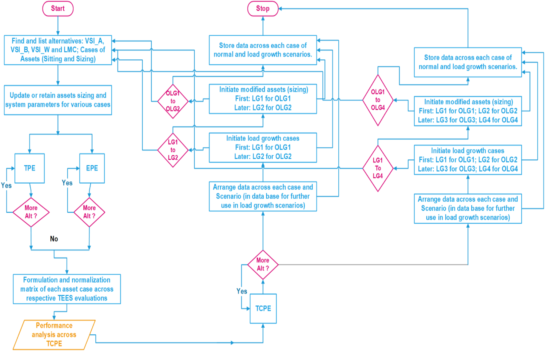
Flow chart of the proposed techno-economic-based sustainable planning (TESP) strategy across multiple planning horizons.
FIGURE 2
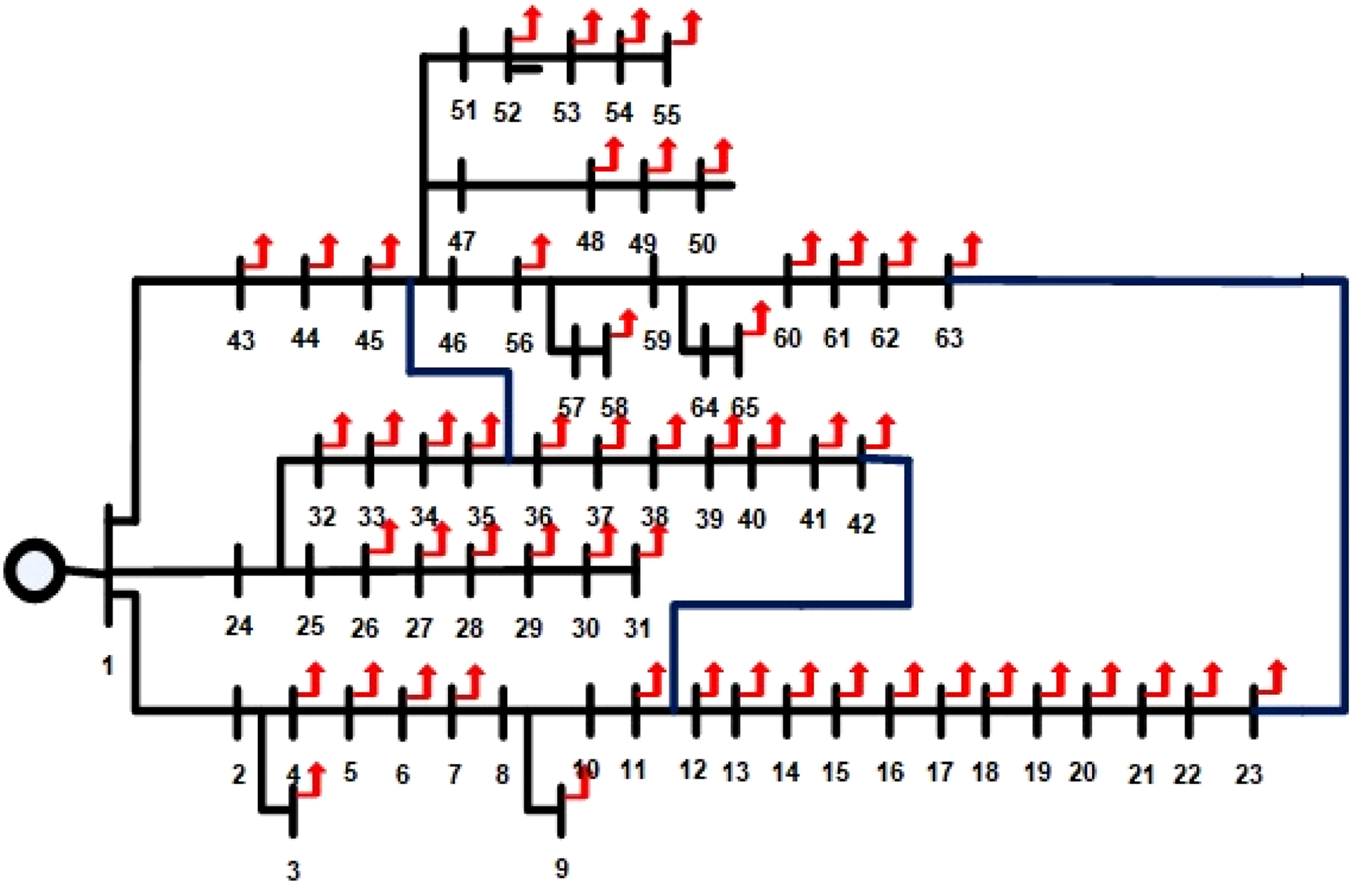
Sixty-five-bus microgrid meshed configured distribution network.
FIGURE 3
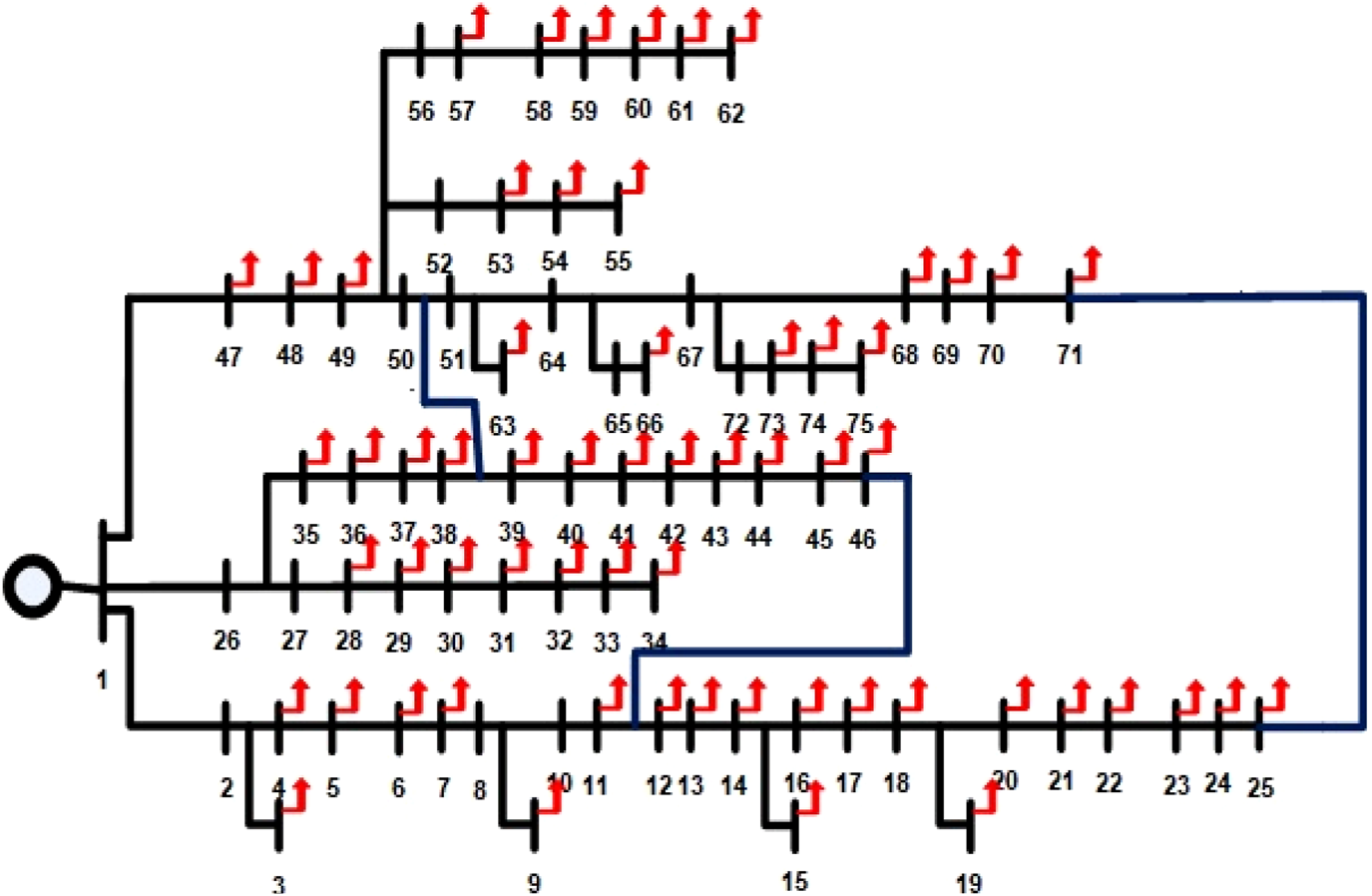
Seventy-five-bus expanded microgrid meshed configured distribution network.
TABLE 1
| S. no. | Technical parameter | Designation | Relationship | Objective |
|---|---|---|---|---|
| 1 | Active power loss (PLoss) (KW) | PLoss | Minimize | |
| 2 | Reactive power loss (QLoss) (KVAR) | QLoss | Minimize | |
| 3 | Active power loss minimization (%) | PLossM | Maximize | |
| 4 | Reactive power loss minimization (%) | QLossM | Maximize | |
| 5 | Penetration of DG by percentage (%) | PDGP | Maximize | |
| 6 | Voltage level (P.U.) | VL | V = 1.0 (reference voltage) | Maximize |
Technical performance evaluation parameters (Kazmi et al., 2021).
TABLE 2
| S. no. | Technical parameter | Designation | Relationship | Objective |
|---|---|---|---|---|
| 1 | Cost of PLoss in millions USD (M$) | CPLoss | Minimize | |
| 2 | Savings of PLoss in millions USD (M$) | SPLoss | Maximize | |
| 3 | Cost of active power for DG ($/MWh) | CDGP | a × where a = 0, b = 20, and c = 0.25 | Minimize |
| 4 | Cost of reactive power for DG ($/MVAR) | CDGQ | ×k, where | Minimize |
Cost-economic performance assessment parameters (Kazmi et al., 2021).
TABLE 3
| Year | Active load (KW) 65 bus | Reactive load (KVAR) 65 bus | Apparent load (KVA) 65 bus | Load growth % 65 bus |
|---|---|---|---|---|
| 2020 | 3949.77 | 1912.97 | 4388.64 | - |
| 2025 | 4512.56 | 2185.54 | 5013.96 | 2.7% |
| 2030 | 5155.54 | 2496.95 | 5728.3813 | 2.7% |
| Year | Active load (KW) 75 bus | Reactive load (KVAR) 75 bus | Apparent load (KVA) 75 bus | Load growth % 75 bus |
| 2020 | 3949.77 | 1912.97 | 4388.64 | - |
| 2023 | 5988.14 | 2899.97 | 6653.39 | 14.9 |
| 2025 | 6315.96 | 3058.84 | 7017.68 | 2.7 |
| 2028 | 10305.94 | 4991.11 | 11452.28 | 17.75 |
| 2030 | 10870 | 5264.24 | 10277.63 | 2.7 |
Load growth values across 65- and 75-bus meshed MGs.
The base case mathematical model is created in MATLAB, and outcomes from the m-file are used to identify the weakest nodes according to the VSI. The outcome-based numericals were collected from the Simulink model setup and were used to perform the simulation The loop currents across TSs will be simulated until became nearly zero and voltages across the various buses became identical, which corresponded to the optimal sizing of assets based on 1% termination criteria. Finally, the obtained values from m-files are implemented in a MATLAB 2018a program, where the suggested multi-criteria sustainable planning technique is assessed using various matrices.
4 Results and discussion
4.1 Case 1 evaluation results
The cases with respective designations, in terms of nomenclature, are illustrated with case (C#) that have been evaluated across the following scenarios (C#/S#):
Case 1 (C1): DG placement in the 65-bus meshed configured microgrid.
Scenario 1 (C1/S1): evaluation across the radial network across two planning horizons of 5 years each of same load growth of 2.7%.
Scenario 2 (C1/S2): evaluation across the mesh network with VSA_A across two planning horizons of 5 years each of same load growth of 2.7%.
Scenario 3 (C1/S3): evaluation across the mesh network with VSA_B across two planning horizons of 5 years each of same load growth of 2.7%.
Scenario 4 (C1/S3): evaluation across the mesh network with VSA_W across two planning horizons of 5 years each of same load growth of 2.7%.
The two load growth horizons for C1 are shown with the following nomenclature:
Normal load:
• 2020
• 2020 optimal reinforcement (2020_O)
Load growth 1 across 5 years with a 2.7% growth rate:
• 2025
• 2025 optimal reinforcement (2025_O)
Load growth 1 across 5 years with a 2.7% growth rate:
• 2030
• 2030 optimal reinforcement (2030_O)
The DG placement and sizing at a 0.9 lagging power factor (LPF) in the 65-bus meshed configured MG evaluated across two planning horizons of 5 years each with a load growth of 2.7% increase per annum are illustrated in Tables 4–6. The 2.7% increment of power demand was chosen to simulate a realistic load growth scenario in the distribution system. This value was based on historical trends and future projections of population growth, urbanization, and industrialization in the area served by the distribution system. The DG siting and sizing based on VSA_A–LMC, VSA_B–LMC and VSA_W–LMC approaches across various parameters are shown in Tables 4–6, respectively. In all those tables, DG units with their capacities and an operating lagging power factor of 0.9 have been illustrated across abovementioned C1 scenarios. The 0.9 power factor was chosen as a typical value for the loads in the distribution system. This value is not necessarily regulated, but it is often used as a benchmark for power factor correction and improvement efforts in distribution systems. It is also a reasonable assumption for modeling and simulation purposes as it represents a moderate level of reactive power demand in the system.
TABLE 4
| DG siting and sizing considering VSA_A- and LMC-based parameters | Normal case 2020 | Optimal case 2020_O | 5-year non-optimal case 2025 | 5-year optimal case 2025_O | 10-year non-optimal case 2030 | 10-year optimal case 2030_O |
|---|---|---|---|---|---|---|
| Active/reactive load (KW + jKVAR) | 3949.77 + j1912.97 | 3949.77 | 4512.64 + j2185.82 | 4512.64 + j2185.82 | 5155.65 + j2497.17 | 5155.65 + j2497.17 |
| + j1912.97 | ||||||
| Grid active/reactive power (KW + jKVAR) | 4010.28 + j1947.6 | 1084.39 + j517.6 | 1650.54 + j7993.66 | 1389.52 + j666.94 | 2036.89 + j982.99 | 1550.84 + 746.78 |
| DG1 bus and size (KW + j KVAR) | — | DG_5 @ 558 + j270.25 | DG_5 @ 558 + j270.25 | DG_5 @ 558 + j270.25 | DG_5 @ 558 + j270.25 | DG_5 @ 558 + j270.25 |
| DG2 @ bus and size (KW + j KVAR) | — | DG_20 @ 441 + j213.59 | DG_20 @ 441 + j213.59 | DG_20 @ 630 + j305.12 | DG_20 @ 630 + j305.12 | DG_20 @ 720 + j348.71 |
| DG3 @ bus and size (KW + j KVAR) | — | DG_40 @ 783 + j379.22 | DG_40 @ 783 + j379.22 | DG_40 @ 855 + j414.1 | DG_40 @ 855 + j414.1 | DG_40 @ 1170 + j566.66 |
| DG4 @ bus and size (KW + j KVAR) | — | DG_52 @ 729 + j353.07 | DG_52@ 729 + j353.07 | DG_52 @ 729 + j353.07 | DG_52 @ 729 + j353.07 | DG_52 @ 810 + j392.3 |
| DG5 @ bus and size (KW + j KVAR) | — | DG_62 @ 414 + j200.51 | DG_62@ 414 + j200.51 | DG_62 @ 414 + j200.51 | DG_62 @ 414 + j200.51 | DG_62 @ 414 + j200.51 |
| Active power loss (KW) | 60.51 | 59.62 | 62.90 | 62.88 | 67.24 | 67.19 |
| Reactive power loss (KVAR) | 34.63 | 21.27 | 24.48 | 24.17 | 28.87 | 28.04 |
DG siting and sizing for a 65-bus meshed MG at 0.9 lagging power factor based on VSA_A and LMC approaches.
TABLE 5
| DG siting and sizing considering VSA_B- and LMC-based parameters | Normal case 2020 | Optimal case 2020_O | 5-year non-optimal case 2025 | 5-year optimal case 2025_O | 10-year non-optimal case 2030 | 10-year optimal case 2030_O |
|---|---|---|---|---|---|---|
| Active/reactive load (KW + jKVAR) | 3949.77 + j1912.97 | 3949.77 + j1912.97 | 4512.64 + j2185.82 | 4512.64 + j2185.82 | 5155.65 + j2497.17 | 5155.65 + j2497.17 |
| Grid active/reactive power (KW + jKVAR) | 4010.28 + j1947.6 | 922.45 + j440.09 | 1488.62 + j716.39 | 1200.61 + j576.59 | 1847.99 + j892.89 | 1442.97 + j696.25 |
| DG1 bus and size (KW + jKVAR) | — | DG_5 @ 270 + j130.77 | DG_5 @ 270 + j130.77 | DG_5 @ 270 + j130.77 | DG_5 @ 270 + j130.77 | DG_5 @ 315 + j152.56 |
| DG2 @ bus and size (KW + jKVAR) | — | DG_14 @ 630 + j305.12 | DG_14 @ 630 + j305.12 | DG_14 @ 720 + j348.71 | DG_14 @ 720 + j348.71 | DG_14 @ 810 + j392.3 |
| DG3 @ bus and size (KW + jKVAR) | — | DG_17 @ 477 + j231.02 | DG_17 @ 477 + j231.02 | DG_17 @ 630 + j305.12 | DG_17 @ 630 + j305.12 | DG_17 @ 720 + j348.71 |
| DG4 @ bus and size (KW + jKVAR) | — | DG_38 @ 855 + j414.1 | DG_38 @ 855 + j414.1 | DG_38 @ 900 + j435.89 | DG_38 @ 900 + j435.89 | DG_38 @ 1080 + j523.07 |
| DG5 @ bus and size (KW + jKVAR) | — | DG_43 @ 855 + j414.1 | DG_43 @ 855 + j414.1 | DG_43 @ 855 + j414.1 | DG_43 @ 855 + j414.1 | DG_43 @ 855 + j414.1 |
| Active power loss (KW) | 60.51 | 59.68 | 62.98 | 62.97 | 67.34 | 67.32 |
| Reactive power loss (KVAR) | 34.63 | 22.23 | 25.68 | 25.36 | 30.31 | 29.82 |
DG siting and sizing for a 65-bus meshed MG at 0.9 lagging power factor based on VSA_B and LMC approaches.
TABLE 6
| DG siting and sizing considering VSA_W-LMC-based parameters | Normal case 2020 | Optimal case 2020_O | 5-year non-optimal case 2025 | 5-year optimal case 2025_O | 10-year non-optimal case 2030 | 10-year optimal case 2030_O |
|---|---|---|---|---|---|---|
| Active/reactive load (KW + jKVAR) | 3949.77 + j1912.97 | 3949.77 + j1912.97 | 4512.64 + j2185.82 | 4512.64 + j2185.82 | 5155.65 + j2497.17 | 5155.65 + j2497.17 |
| Grid active/reactive power (KW + jKVAR) | 4010.28 + j1947.6 | 1534.42 + j736.06 | 2100.59 + j1012.34 | 1677.56 + j807 | 2324.93 + j1123.1 | 1856.9 + j895.88 |
| DG1 bus and size (KW + jKVAR) | — | DG_5 @ 360 + j174.36 | DG_5 @ 360 + j174.36 | DG_5 @ 423 + j204.87 | DG_5 @ 423 + 204.87 | DG_5 @ 468 + 226.66 |
| DG2 @ bus and size (KW + jKVAR) | — | DG_17 @ 270 + j130.77 | DG_17 @ 270 + j130.77 | DG_17 @ 405 + j196.15 | DG_17 @ 405 + j196.15 | DG_17 @ 423 + j204.87 |
| DG3 @ bus and size (KW + jKVAR) | — | DG_38 @ 585 + j283.33 | DG_38 @ 585 + j283.33 | DG_38 @ 675 + j326.92 | DG_38 @ 675 + j326.92 | DG_38 @ 675 + j326.92 |
| DG4 @ bus and size (KW + jKVAR) | — | DG_42 @ 630 + j305.12 | DG_42 @ 630 + j305.12 | DG_42 @ 675 + j326.92 | DG_42 @ 675 + j326.92 | DG_42 @ 720 + j348.71 |
| DG5 @ bus and size (KW + jKVAR) | — | DG_62 @ 630 + j305.12 | DG_62 @ 630 + j305.12 | DG_62 @ 720 + j348.71 | DG_62 @ 720 + j348.71 | DG_62 @ 810 + j392.3 |
| Active power loss (KW) | 60.51 | 59.65 | 62.95 | 62.92 | 67.28 | 67.25 |
| Reactive power loss (KVAR) | 34.63 | 21.79 | 25.22 | 24.75 | 29.5 | 28.93 |
DG siting and sizing for a 65-bus meshed MG at 0.9 lagging power factor based on VSA_W and LMC approaches.
For the VSA_A–LMC-based approach, the normal scenario in both cases is the same, such as the year 2020 scenario. Load has increased linearly at 2.7 percent per year in the actual model after 3 years, as well as due to the addition of new load programs. Because the load has changed and the DG capacity has remained the same as in scenario 2020, DG values for scenario 2023 will need to be adjusted for this model after 3 years. The DG capacity has been re-optimized to meet the model’s current requirement. According to scenario 2020, weak nodes would remain the same.
Similarly, for VSA_B–LMC- and VSA_W–LMC-based approach variants, load has increased linearly at 2.7 percent per year in the actual model after 3 years, as well as due to the addition of new load programs. Because the load has changed and the DG capacity has remained the same as in scenario 2020, DG values for scenario 2023 will need to be optimized for this model after 3 years. The DG capacity has also been re-optimized to meet the model’s current requirement. All three VSIs were performed according to their respective criteria in order to increase the voltage profile and maximize the model’s technical characteristics.
In Figure 4, case 1 shows an active power loss trend across two planning horizons (accumulatively 10 years) in the 65-bus meshed configured MG-based distribution network. It can be observed that the active power losses have reduced in meshed configured approaches in C1, scenarios 2–4 compared to the radial counterpart in scenario 1.
FIGURE 4
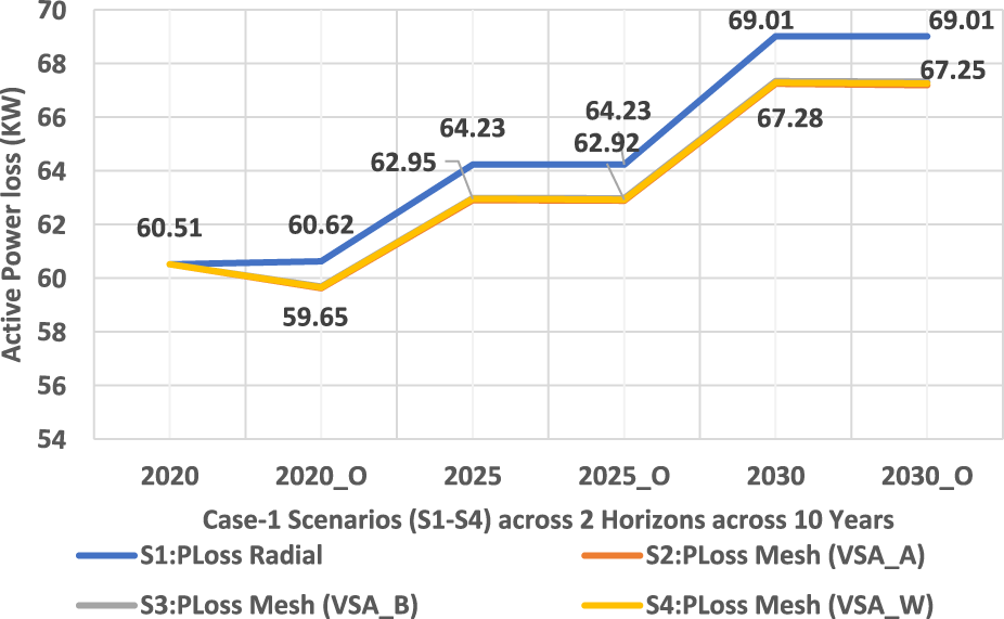
Active power loss trend across two planning horizons in the 65-bus meshed configured MG-based distribution network.
Figure 5 and Figure 6 show that a substantial improvement is active and prominent in reactive power loss minimization across all scenarios of C1. The reason being that reactive power loss is high because the distribution network is laid underground rather than overhead cables. Figure 7 shows that each VSI enhanced the voltage profile of the network according to its own specifications, and that all VSIs are significantly superior to a simple interconnected network. After maximizing the value of DG penetration in accordance with the policy, the voltage of each node is brought to unity. For this scenario, a new optimized model has been acquired. Figure 8 shows a phenomenal reduction in the cost of active power losses and an increase in savings.
FIGURE 5
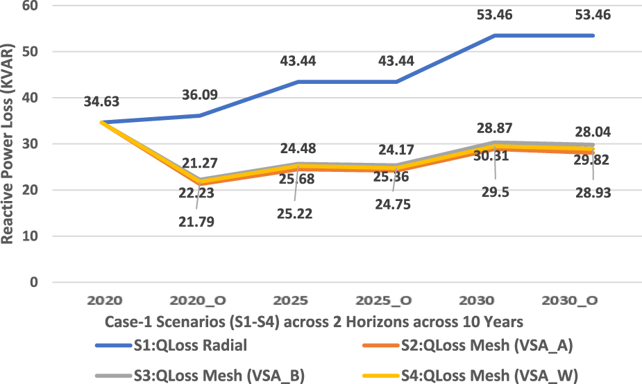
Reactive power loss trend across two planning horizons in the 65-bus meshed configured MG-based distribution network.
FIGURE 6
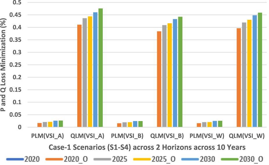
Active and reactive power loss minimization trends across two planning horizons in the 65-bus meshed configured MG-based distribution network.
FIGURE 7
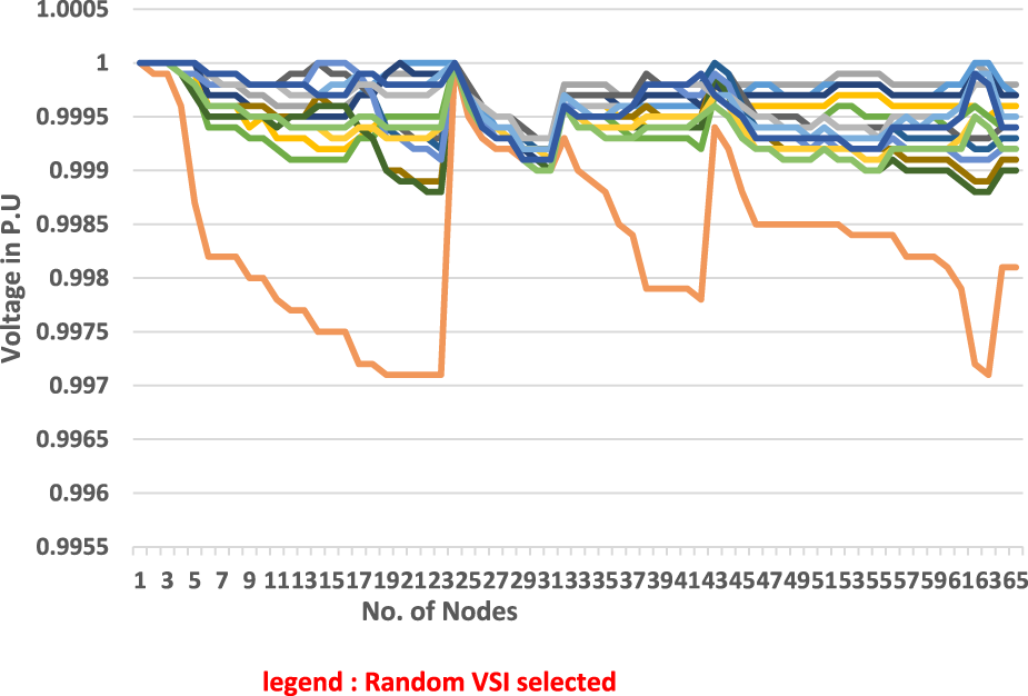
Voltage profile trend across two planning horizons in the 65-bus meshed configured MG-based distribution network.
FIGURE 8
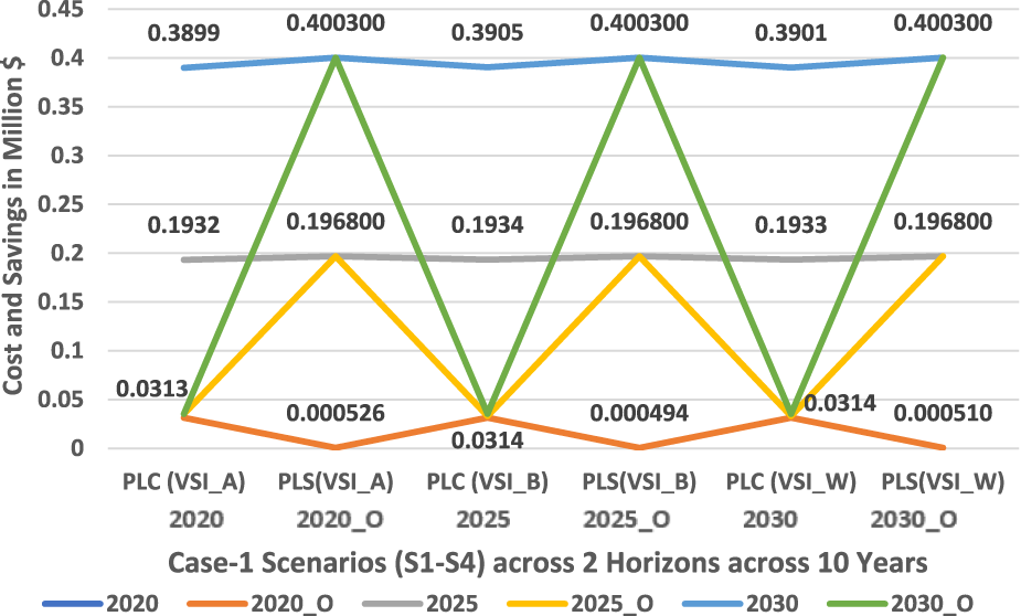
Cost of active power losses and savings trend across two planning horizons in the 65-bus meshed configured MG-based distribution network.
4.2 Case 2 evaluation results
The cases with respective designations, in terms of nomenclature, are illustrated with case (C#) that have been evaluated across the following scenarios (C#/S#):
Case 2 (C2): DG placement in the 75-bus meshed configured microgrid.
Scenario 1 (C2/S1): evaluation across the radial network across four different planning horizons of 5 years each of various load growth levels.
Scenario 2 (C2/S2): evaluation across the mesh network with VSA_A across four different planning horizons of various load growth levels.
Scenario 3 (C2/S3): evaluation across the mesh network with VSA_B across four different planning horizons of various load growth levels.
Scenario 4 (C2/S3): evaluation across the mesh network with VSA_W across four different planning horizons of various load growth levels.
The four load growth horizons for C2 are shown with the following nomenclature:
Normal load:
• 2020
• 2020 optimal reinforcement (2020_O)
Load growth 1 across 3 years with a 14.9% growth rate:
• 2023
• 2023 optimal reinforcement (2023_O)
Load growth 2 across 2 years with a 2.7% growth rate:
• 2025
• 2025 optimal reinforcement (2025_O)
Load growth 1 across 3 years with a 17.75% growth rate:
• 2028
• 2028 optimal reinforcement (2028_O)
Load growth 4 across 2 years with a 2.7% growth rate:
• 2030
• 2030 optimal reinforcement (2030_O)
The DG placement and sizing at 0.9 lagging power factor in the 75-bus meshed configured MG evaluated across four planning horizons of 2–3 years each with a variable expansion-based load growth increase per annum are illustrated in Tables 7–9. The DG siting and sizing based on VSA_A–LMC-, VSA_B–LMC-, and VSA_W–LMC approaches are illustrated across various parameters in Tables 7–9, respectively. In all those tables, DG units with their capacities and an operating lagging power factor (LPF) of approximately 0.9 have been illustrated across abovementioned C2 scenarios. All the data are provided in a self-explanatory manner.
TABLE 7
| DG place/size considering VSA_A–LMC-based parameters | Normal case 2020 | Optimal case 2020_O | 3-year non-optimal case 2023 | 3-year optimal case 2023_O | 5-year non-optimal case 2025 | 5-year optimal case 2025_O | 8-year non-optimal case 2028 | 8-year optimal case 2028_O | 10-year non-optimal case 2030 | 10-year optimal case 2030_O |
|---|---|---|---|---|---|---|---|---|---|---|
| Active/reactive load (KW + jKVAR) | 3949.77 + j1912.97 | 2196.99 + j1065.2 | 3151.17 KW + j1529.96 KVAR | 2196.99 KW + j1065.18 KVAR | 3221.19 KW + j1564.47 KVAR | 2240.01 KW + j 1086.63 KVAR | 7303.55 KW + j3773.83 KVAR | 2521.24 KW + j1221.49 KVAR | 7882.44 KW + j 4085.16 KVAR | 2541.47 KW + j 1255.03 KVAR |
| Grid active/reactive power (KW + jKVAR) | 4010.28 + j1947.6 | 5988.14 +j2899.97 | 5988.14 KW + j2899.97 KVAR | 5988.14 KW + j2899.97 KVAR | 6315.96 KW + j3058.84 KVAR | 6315.96 KW + j 3058.84 KVAR | 10305.94 KW + j4991.11 KVAR | 10305.94 KW + j 4991.11 KVAR | 10870 KW + j 5264.24 KVAR | 10870 KW + j 5264.24 KVAR |
| DG1 bus and size (KW + jKVAR) | — | DG_5 @540 + j261.53 | DG_5 = 558 KW + j270.25 KVAR | DG_5 = 540 KW + j261.53 KVAR | DG_5 = 558 KW + j270.25 KVAR | DG_5 = 540 KW + j261.53 KVAR | DG_5 @ 558 KW + j 270.25 KVAR | DG_5 @ 585 KW + j283.33 KVAR | DG_5 @ 558 KW + j 270.25 KVAR | DG_5 @ 630 KW + j305.12 KVAR |
| DG2 @ bus and size (KW + jKVAR) | — | DG_22 @ 990 + j479.48 | DG_22 = 441 KW + j213.59 KVAR | DG_22 = 990 KW + j479.48 KVAR | DG_22 = 630 KW + j305.12 KVAR | DG_22 = 990 KW + j479.48 KVAR | DG_22 @ 630 KW + j305.12 KVAR | DG_22 @ 1350 KW + j653.84 KVAR | DG_22 @ 630 KW + j305.12 KVAR | DG_22 @ 1350 KW + j653.84 KVAR |
| DG3 @ bus and size (KW + jKVAR) | — | DG_44 @ 855 + j414.1 | DG_44 = 783 KW + j379.22 KVAR | DG_44 = 855 KW + j414.1 KVAR | DG_44 = 855 KW + j414.1 KVAR | DG_44 = 1008 KW + j488.2 KVAR | DG_44 @ 855 KW + j414.1 KVAR | DG_44 @ 1620 KW + j784.6 KVAR | DG_44 @ 855 KW + j414.1 KVAR | DG_44 @ 1620 KW + j784.6 KVAR |
| DG4 @ bus and size (KW + jKVAR) | — | DG_57@ 1080 +j523.07 | DG_57 = 729 KW + j353.07 KVAR | DG_57 = 1080 KW + j523.07 KVAR | DG_57 = 729 KW + j353.07 KVAR | DG_57 = 1215 KW + j588.45 KVAR | DG_57 @ 729 KW + j353.07 KVAR | DG_57 @ 3870 KW + j1874.3 KVAR | DG_57 @ 729 KW + j353.07 KVAR | DG_57 @ 4293 KW + j2079.2 KVAR |
| DG5 @ bus and size (KW + jKVAR) | — | DG_70 @ 414 + j200.51 | DG_70 = 414 KW + j.51 KVAR | DG_70 = 414 KW + j200.51 KVAR | DG_70 = 414 KW + j200.51 KVAR | DG_70 = 414 KW + j200.51 KVAR | DG_70 @ 414 KW + j200.51 KVAR | DG_70 @ 540 KW + j261.53 KVAR | DG_70 @ 414 KW + j 200.51 KVAR | DG_70 @ 630 KW + j305.12 KVAR |
| Active power loss (KW) | 60.51 | 87.85 | 88.03 KW | 87.85 KW | 91.23 KW | 91.05 KW | 183.61 KW | 180.3 KW | 198.44 KW | 194.47 KW |
| Reactive power loss (KVAR) | 34.63 | 43.9 | 46.63 KVAR | 43.9 KVAR | 48.68 KVAR | 45.96 KVAR | 325.77 KVAR | 87.98 KVAR | 363.97 KVAR | 118.67 KVAR |
DG siting and sizing for a 75-bus meshed MG at 0.9 lagging power factor based on VSA_A and LMC approaches.
TABLE 8
| DG place/size considering VSA_A-LMC-based parameters | Normal case 2020 | Optimal case 2020_O | 3-year non-optimal case 2023 | 3-year optimal case 2023_O | 5-year non-optimal case 2025 | 5-year optimal case 2025_O | 8-year non-optimal case 2028 | 8-year optimal case 2028_O | 10-year non-optimal case 2030 | 10-year optimal case 2030_O |
|---|---|---|---|---|---|---|---|---|---|---|
| Active/reactive load (KW + jKVAR) | 3949.77 + j1912.97 | 2989.35 KW + j1454.05 KVAR | 3320.48 KW + j1616.58 KVAR | 2116.2 KW + j1028.77 KVAR | 2447.26 KW + j1190.52 KVAR | 2195.26 KW + j1068.28 KVAR | 6277.59 KW + j3049.41 KVAR | 2865.56 KW + j1613.34 KVAR | 3444.16 KW + j1704.39 KVAR | 2832.1 KW + j1401.92 KVAR |
| Grid active/reactive power (KW + jKVAR) | 4010.28 + j1947.6 | 5988.14 KW + j2899.97 KVAR | 6315.96 KW + j 3058.84 KVAR | 5988.14 KW + j 2899.97 KVAR | 6315.96 KW + j 3058.84 KVAR | 6315.96 KW + j 3058.84 KVAR | 10305.94 KW + j 4991.11 KVAR | 10305.94 KW + j4991.11KVAR | 10870 KW + j5264.24 KVAR | 10870 KW + j5264.24 KVAR |
| DG1 bus and size (KW + jKVAR) | — | DG_5 = 270 KW + j130.77 KVAR | DG_5 = 270 KW + j130.77 KVAR | DG_5 = 270 KW + j130.77 KVAR | DG_5 = 270 KW + j130.77 KVAR | DG_5 = 270 KW + j 130.77 KVAR | DG_5 = 270 KW + j130.77 KVAR | DG_5 = 270 KW + j130.77 KVAR | DG_5 = 270 KW + j130.77 KVAR | DG_5 = 315 KW + j152.56 KVAR |
| DG2 @ bus and size (KW + jKVAR) | — | DG_14 = 630 KW + j305.12 KVAR | DG_14 = 630 KW + j 305.12 KVAR | DG_14 = 765 KW + j370.51 KVAR | DG_14 = 765 KW + j370.51 KVAR | DG_14 = 792 KW + j383.58 KVAR | DG_14 = 792 KW + j 383.58 KVAR | DG_14 = 783 KW + j 379.22 KVAR | DG_14 = 783 KW + j379.22 KVAR | DG_14 = 765 KW + j370.51 KVAR |
| DG3 @ bus and size (KW + jKVAR) | — | DG_18 = 477 KW + j231.02 KVAR | DG_18 = 477 KW + j231.02 KVAR | DG_18 = 1035 KW + j501.27 KVAR | DG_18 = 1035 KW + j501.27 KVAR | DG_18 = 1080 KW + j 523.07 KVAR | DG_18 = 1080 KW + j523.07 KVAR | DG_18 = 1800 KW + j871.78 KVAR | DG_18 = 1800 KW + j871.78 KVAR | DG_18 = 1890 KW + j915.37 KVAR |
| DG4 @ bus and size (KW + jKVAR) | — | DG_42 = 855 KW + j414.1 KVAR | DG_42 = 855 KW + j414.1 KVAR | DG_42 = 1035 KW + j501.27 KVAR | DG_42 = 1035 KW + j501.27 KVAR | DG_42 = 1080 KW + j 523.07 KVAR | DG_42 = 1080 KW + j523.07 KVAR | DG_42 = 2070 KW + j1002.5 KVAR | DG_42 = 2070 KW + j1002.5 KVAR | DG_42 = 2295 KW + j1111.5 KVAR |
| DG5 @ bus and size (KW + jKVAR) | — | DG_47 = 855 KW + j414.1 KVAR | DG_47 = 855 KW + j414.1 KVAR | DG_47 = 855 KW + j 414.1 KVAR | DG_47 = 855 KW + j414.1 KVAR | DG_47 = 990 KW + j 479.48 KVAR | DG_47 = 990 KW + j479.48 KVAR | DG_47 = 2700 KW + j1307.7 KVAR | DG_47 = 2700 KW + j1307.7 KVAR | DG_47 = 2970 KW + j1438.4 KVAR |
| Active power loss (KW) | 60.51 | 88.21 KW | 91.52 KW | 88.06 KW | 91.30 KW | 91.30 KW | 183.65 KW | 182.62 KW | 197.16 KW | 197.10 KW |
| Reactive power loss (KVAR) | 34.63 | 49.19 KVAR | 52.85 KVAR | 46.72 KVAR | 49.60 KVAR | 49.41 KVAR | 98.27 KVAR | 86.13 KVAR | 132.12 KVAR | 126.02 KVAR |
DG siting and sizing for a 75-bus MG at 0.9 lagging power factor based on VSA_B and LMC approaches.
TABLE 9
| DG place/size considering VSA_A–LMC-based parameters | Normal case 2020 | Optimal case 2020_O | 3-year non-optimal case 2023 | 3-year optimal case 2023_O | 5-year non-optimal case 2025 | 5-year optimal case 2025_O | 8-year non-optimal case 2028 | 8-year optimal case 2028_O | 10-year non-optimal case 2030 | 10-year optimal case 2030_O |
|---|---|---|---|---|---|---|---|---|---|---|
| Active/reactive load (KW + jKVAR) | 3949.77 + j1912.97 | 3601.33 KW + j1750.14 KVAR | 3932.46 KW + j1912.67 KVAR | 2566.13 KW + j 1245.93 KVAR | 2897.19 KW + j1407.6 KVAR | 2609.18 KW + j1267.92 KVAR | 6691.28 KW + j3246.28 KVAR | 4638.37 KW + j2273.25 KVAR | 5216.95 KW + j2550.29 KVAR | 4874.9 KW + j2384.33 KVAR |
| Grid active/reactive power (KW + jKVAR) | 4010.28 + j1947.6 | 5988.14 KW + j2899.97 KVAR | 6315.96 KW + j3058.84 KVAR | 5988.14 KW + j2899.97 KVAR | 6315.96 KW + j3058.84 KVAR | 6315.96 KW + j3058.84 KVAR | 10305.94 KW + j4991.11 KVAR | 10305.94 KW + j4991.11 KVAR | 10870 KW + j5264.24 KVAR | 10870 KW + j5264.24 KVAR |
| DG1 bus and size (KW + jKVAR) | — | DG_5 = 360 KW + j174.36 KVAR | DG_5 = 360 KW + j174.36 KVAR | DG_5 = 423 KW + j204.87 KVAR | DG_5 = 423 KW + j204.87 KVAR | DG_5 = 423 KW + j204.87 KVAR | DG_5 = 423 KW + j204.87 KVAR | DG_5 = 405 KW + j196.15 KVAR | DG_5 = 405 KW + j196.15 KVAR | DG_5 = 387 KW + j187.43 KVAR |
| DG2 @ bus and size (KW + jKVAR) | — | DG_18 = 270 KW + j 130.77 KVAR | DG_18 = 270 KW + j130.77 KVAR | DG_18 = 540 KW + j261.53 KVAR | DG_18 = 540 KW + j 261.53 KVAR | DG_18 = 630 KW + j305.12 KVAR | DG_18 = 630 KW + j305.12 KVAR | DG_18 = 837 KW + j405.38 KVAR | DG_18 = 837 KW + j405.38 KVAR | DG_18 = 855 KW + j414.1 KVAR |
| DG3 @ bus and size (KW + jKVAR) | — | DG_42 = 585 KW + j283.33 KVAR | DG_42 = 585 KW + j283.33 KVAR | DG_42 = 882 KW + j427.17 KVAR | DG_42 = 882 KW + j427.17 KVAR | DG_42 = 945 KW + j457.68 KVAR | DG_42 = 945 KW + j457.68 KVAR | DG_42 = 1395 KW + j675.63 KVAR | DG_42 = 1395 KW + j675.63 KVAR | DG_42 = 1620 KW + j784.6 KVAR |
| DG4 @ bus and size (KW + jKVAR) | — | DG_46 = 630 KW + j305.12 KVAR | DG_46 = 630 KW + j305.12 KVAR | DG_46 = 720 KW + j348.71 KVAR | DG_46 = 720 KW + j348.71 KVAR | DG_46 = 810 KW + j392.3 KVAR | DG_46 = 810 KW + j392.3 KVAR | DG_46 = 1350 KW + j653.84 KVAR | DG_46 = 1350 KW + j653.84 KVAR | DG_46 = 1395 KW + j675.63 KVAR |
| DG5 @ bus and size (KW + jKVAR) | — | DG_70 = 630 KW + j305.12 KVAR | DG_70 = 630 KW + j305.12 KVAR | DG_70 = 945 KW + j 457.68 KVAR | DG_70 = 945 KW + j457.68 KVAR | DG_70 = 990 KW + j479.48 KVAR | DG_70 = 990 KW479.48 KVAR | DG_70 = 1863 KW + j902.29 KVAR | DG_70 = 1863 KW + j902.29 KVAR | DG_70 = 1935 KW + j937.16 KVAR |
| Active power loss (KW) | 60.51 | 88.19 KW | 91.50 KW | 87.99 KW | 91.23 KW | 91.22 KW | 183.34 KW | 182.43 KW | 196.95 KW | 196.90 KW |
| Reactive power loss (KVAR) | 34.63 | 48.87 KVAR | 52.53 KVAR | 45.92 KVAR | 48.72 KVAR | 48.53 KVAR | 94.62 KVAR | 85.02 KVAR | 119.34 KVAR | 119.01 KVAR |
DG siting and sizing for a 75-bus meshed MG at 0.9 lagging power factor based on VSA_W and LMC approaches.
In Figure 9, case 2 shows an active power loss trend across four planning horizons (accumulatively 10 years) in the 75-bus meshed configured MG-based distribution network. It can be observed that the active power losses have reduced in meshed configured approaches in C2, scenarios 2–4 compared to the radial counterpart in scenario 2.
FIGURE 9
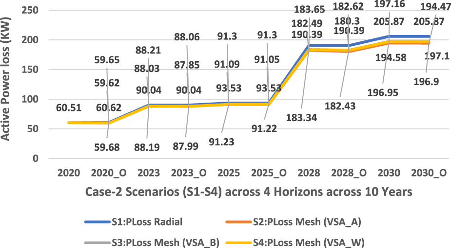
Active power loss trend across four planning horizons in the 75-bus meshed configured MG-based distribution network.
Figure 10 and Figure 11 show that a substantial improvement is active and prominent in reactive power loss minimization across all scenarios of C2 and is quite greater than that in C1 and respective scenarios. The reason being that reactive power loss is high because the distribution network is laid underground rather than overhead cables. Figure 12 shows that each VSI enhanced the voltage profile of the network according to its own specifications and all VSIs are significantly superior to a simple interconnected network. After maximizing the value of DG penetration in accordance with the policy, the voltage of each node is brought to unity. For scenario, a new optimized model has been acquired. Figure 13 shows a phenomenal reduction in the cost of active power losses and an increase in savings.
FIGURE 10
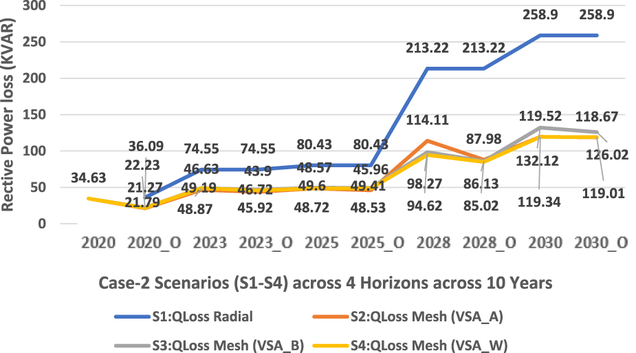
Reactive power loss trend across four planning horizons in the 75-bus meshed configured MG-based distribution network.
FIGURE 11
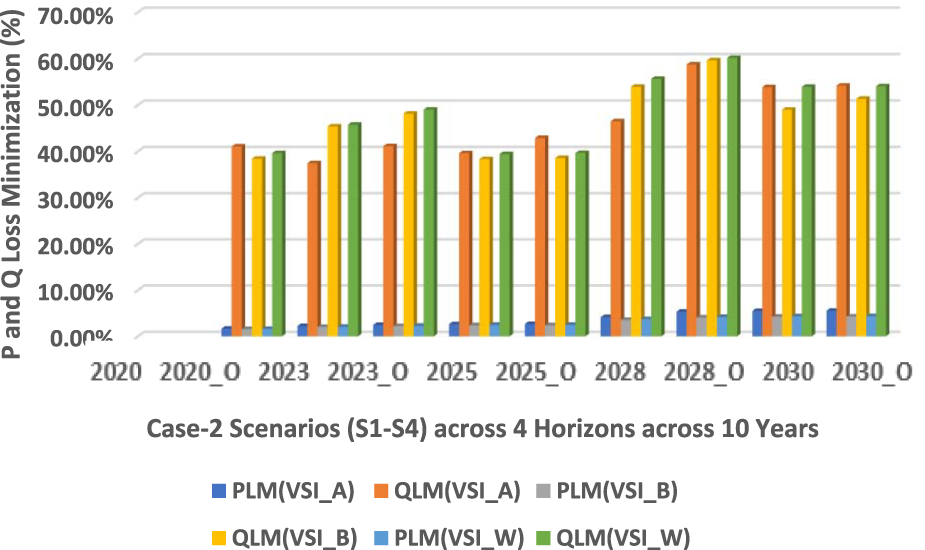
Active and reactive power loss minimization trends across four planning horizons in the 75-bus meshed configured MG-based distribution network.
FIGURE 12
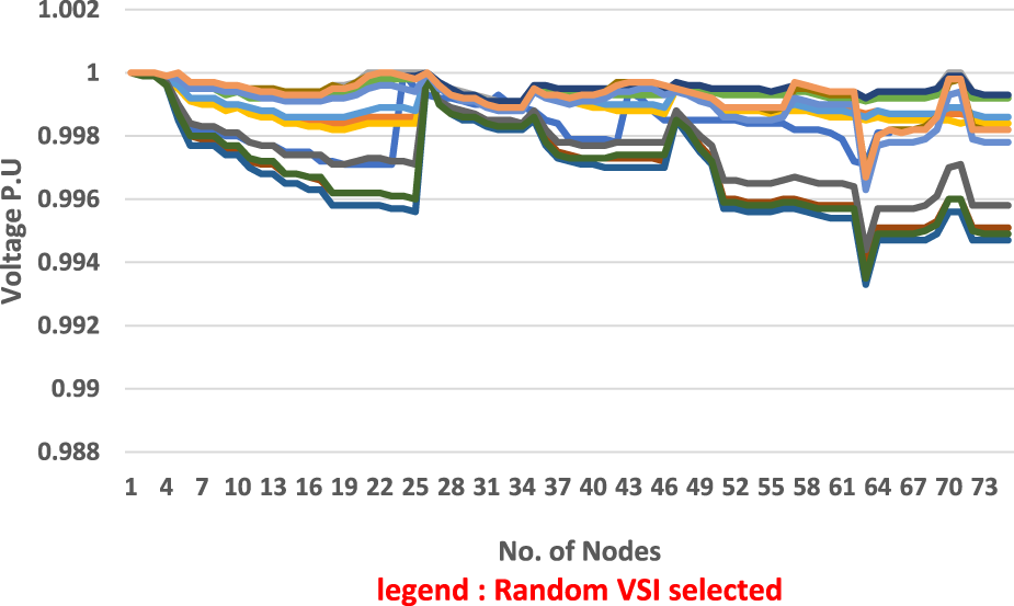
Voltage profile trend across four planning horizons in the 75-bus meshed configured MG-based distribution network.
FIGURE 13
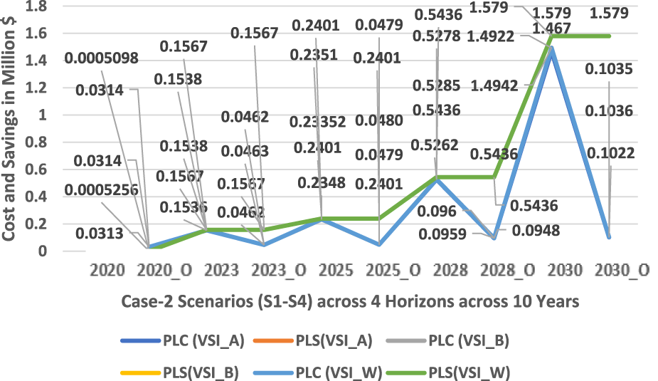
Cost of active power losses and savings trend across four planning horizons in the 75-bus meshed configured MG-based distribution network.
Further examination in Figure 10 and Figure 11 reveals that both active and reactive power losses are considerably minimized in C2 across all scenarios, surpassing the results of case 1 (C1). The higher reactive power loss in the baseline scenario is attributed to the network’s underground cabling system. In Figure 12, the implementation of various voltage stability indices (VSIs) has been shown to significantly improve the voltage profile over a simple interconnected network, bringing each node’s voltage closer to unity after the integration of maximum distributed generation (DG) penetration according to the set policy.
The obtained results in all situations were compared with the existing literature, and a close approximation was observed in the results, especially in evaluating contradictory criteria with cases of load increase over numerous planning horizons. It is also observed that fixed load growth by percentages does not capture the realistic pictures across medium horizons of 5 years, as evident from evaluated case 1. It is observed from evaluated case 2 that small planning horizons with variable load growth levels capture the requirements of expansion-based planning efficiently with the fixed counterpart.
5 Conclusion
Within the smart grid paradigm, current distribution networks aim to enhance reliability and interconnected topology while meeting diverse performance requirements. This study introduces a TESP (transmission expansion planning) strategy to address grid planning challenges. The proposed multi-stage comprehensive strategy employs voltage stability assessment indices (VSA_A, VSA_B, and VSA_W) and a load margin constraint (LMC) to assess and optimize the positioning and sizing of distributed generation (DG) assets. The evaluation of potential solutions considers technical and economic performance indicators across two load growth scenarios spanning 10 years. The TESP technique is tested on two variants of distribution grids (65-bus and 75-bus) with different load growth patterns. The results are compared with the existing literature, demonstrating close alignment, especially in assessing performance amid conflicting standards across various planning horizons. Notably, fixed load growth percentages may not accurately depict realistic scenarios over five-year planning horizons, as evident from case 1. Conversely, smaller planning horizons with variable load growth levels effectively address expansion-based planning needs, reducing assessment time and sensitivity analysis. Additionally, the TESP method offers a wide range of trade-off options for performance indicators, making it a valuable planning tool for academics and distribution system planners in interconnected distribution networks.
Statements
Data availability statement
The original contributions presented in the study are included in the article/Supplementary Material; further inquiries can be directed to the corresponding author.
Author contributions
AA: conceptualization, data curation, funding acquisition, resources, software, validation, writing–original draft, and writing–review and editing.
Funding
The author(s) declare financial support was received for the research, authorship, and/or publication of this article. The authors extend their appreciation to the Deanship of Scientific Research, Majmaah University, Saudi Arabia, for funding this research work through project number R-2023-192.
Conflict of interest
The author declares that the research was conducted in the absence of any commercial or financial relationships that could be construed as a potential conflict of interest.
Publisher’s note
All claims expressed in this article are solely those of the authors and do not necessarily represent those of their affiliated organizations, or those of the publisher, the editors, and the reviewers. Any product that may be evaluated in this article, or claim that may be made by its manufacturer, is not guaranteed or endorsed by the publisher.
References
1
Ali F. Nazir Z. Inayat U. Ali S. M. (2019). “Infrastructure of south Korean electric power system and potential barriers for the implementation of smart grid: a review,” in International Conference on Innovative Computing (ICIC), Japan, August 29-31, 2023 (IEEE), 1–7.
2
Al-Sharafi A. Sahin A. Z. Ayar T. Yilbas B. S. (2017). Techno-economic analysis and optimization of solar and wind energy systems for power generation and hydrogen production in Saudi Arabia. Int. J. Renew. Sust. Ener Rev.69, 33–49. 10.1016/j.rser.2016.11.157
3
Alvarez-Herault M.-C. N’Doye N. Gandioli C. Hadjsaid N. Tixador P. (2015). Meshed distribution network vs reinforcement to increase the distributed generation connection. Sustain. Energy, Grids Netw.1, 20–27. 10.1016/j.segan.2014.11.001
4
Arshad M. A. Ahmad S. Afzal M. J. Kazmi S. A. A. (2018). “Scenario based performance evaluation of loop configured microgrid under load growth using multi-criteria decision analysis,” in Proceedings of the 14th International Conference on Emerging Technologies (ICET), Islamabad, 21–22 Nov, 2018 (IEEE), 1–6.
5
Chen L. Deng X. Xia F. Chen H. Liu C. Chen Q. et al (2021). A techno-economic sizing approach for medium-low voltage DC distribution system. IEEE Trans. Appl. Supercond.31 (8), 1–6. 10.1109/tasc.2021.3101773
6
Das B. K. Hoque N. Mandal S. Pal T. K. Raihan M. A. (2017). A techno-economic feasibility of a stand-alone hybrid power generation for remote area application in Bangladesh. Energy134 (1), 775–788. 10.1016/j.energy.2017.06.024
7
Das S. K. Sarkar S. Das D. (2022). Performance enhancement of grid-connected distribution networks with maximum penetration of optimally allocated distributed generation under annual load variation. Arabian J. Sci. Eng.47 (11), 14809–14839. 10.1007/s13369-022-06951-x
8
Evangelopoulos V. A. Georgilakis P. Hatziargyriou N. D. (2016). Optimal operation of smart distribution networks: a review of models, methods and future research. Electr. Power Syst. Res.140, 95–106. 10.1016/j.epsr.2016.06.035
9
Gholami K. Islam M. R. Rahman M. M. Azizivahed A. Fekih A. (2022). State-of-the-art technologies for volt-var control to support the penetration of renewable energy into the smart distribution grids. Energy Rep.8, 8630–8651. 10.1016/j.egyr.2022.06.080
10
Javaid B. Arshad M. A. Ahmad S. Kazmi S. A. A. (2019). “Comparison of different multi criteria decision analysis techniques for performance evaluation of loop configured Micro grid,” in Proceedings of the 2019 2nd International Conference on Computing, Mathematics and Engineering Technologies (iCoMET), Sukkur, Pakistan, 30–31 January 2019 (IEEE), 1–7.
11
Kazmi S. A. A. Ahmad H. W. Shin D. R. (2019). A new improved voltage stability assessment index-centered integrated planning approach for multiple asset placement in mesh distribution systems. Energies12, 3163. 10.3390/en12163163
12
Kazmi S. A. A. Ameer Khan U. Ahmad W. Hassan M. Ibupoto F. A. Bukhari S. B. A. et al (2021). Multiple (TEES)-Criteria-Based sustainable planning approach for mesh-configured distribution mechanisms across multiple load growth horizons. Energies14, 3128. 10.3390/en14113128
13
Kazmi S. A. A. Shahzaad M. K. Shin D. R. (2017b). Voltage stability index for distribution network connected in loop configuration. IETE J. Res.63, 281–293. 10.1080/03772063.2016.1257376
14
Kazmi S. A. A. Shahzad M. K. Shin D. R. (2017a). Multi-objective planning techniques in distribution networks: a composite review. Energies10, 208. 10.3390/en10020208
15
Khan S. N. Kazmi S. A. A. Altamimi A. Khan Z. A. Alghassab M. A. (2022). Smart distribution mechanisms—Part I: from the perspectives of planning. Sustainability14 (23), 16308. 10.3390/su142316308
16
Mahmoud P. H. A. Phung D. H. Vigna K. R. (2017). A review of the optimal allocation of distributed generation: objectives, constraints, methods, and algorithms. Renew. Sustain. Energy Rev.75, 293–312. 10.1016/j.rser.2016.10.071
17
Mallala B. Dwivedi D. (2022). Salp swarm algorithm for solving optimal power flow problem with thyristor-controlled series capacitor. J. Electron. Sci. Technol.20 (2), 100156. 10.1016/j.jnlest.2022.100156
18
Mallala B. Venkata Prasad P. Palle K. (2023). “Multi-objective optimization with practical constraints using AALOA,” in International Conference on Information and Communication Technology for Intelligent Systems, Singapore, APRIL 4 – 5, 2024 (Springer Nature Singapore), 165–177.
19
Modarresi J. Gholipour E. Khodabakhshian A. (2016). A comprehensive review of the voltage stability indices. Renew. Sustain Energy Rev.63, 1–12. 10.1016/j.rser.2016.05.010
20
Paliwal P. (2021). Comprehensive analysis of distributed energy resource penetration and placement using probabilistic framework. IET Renew. Power Gener.15 (4), 794–808. 10.1049/rpg2.12069
Summary
Keywords
power system, renewable energy, distributed generation, energy, energy consumption
Citation
Altamimi A (2024) Techno-economic evaluation of meshed distribution network planning with load growth and expansion with multiple assets across multiple planning horizons. Front. Energy Res. 12:1353071. doi: 10.3389/fenrg.2024.1353071
Received
09 December 2023
Accepted
03 January 2024
Published
18 January 2024
Volume
12 - 2024
Edited by
Ch. Rami Reddy, Chonnam National University, Republic of Korea
Reviewed by
Nagi Reddy B., Vignana Bharathi Institute of Technology, India
Balasubbareddy Mallala, Chaitanya Bharathi Institute of Technology, India
Updates
Copyright
© 2024 Altamimi.
This is an open-access article distributed under the terms of the Creative Commons Attribution License (CC BY). The use, distribution or reproduction in other forums is permitted, provided the original author(s) and the copyright owner(s) are credited and that the original publication in this journal is cited, in accordance with accepted academic practice. No use, distribution or reproduction is permitted which does not comply with these terms.
*Correspondence: Abdullah Altamimi, a.altmimi@mu.edu.sa
Disclaimer
All claims expressed in this article are solely those of the authors and do not necessarily represent those of their affiliated organizations, or those of the publisher, the editors and the reviewers. Any product that may be evaluated in this article or claim that may be made by its manufacturer is not guaranteed or endorsed by the publisher.