Research on wire icing simulation technology considering the weights of meteorological elements

Wire icing seriously threatens the safety and reliability of power systems. Strengthening the simulation study of icing thickness is crucial for disaster prevention and mitigation, as well as the adjustment of power system operation strategies. The meteorological elements, including air temperature, precipitation and wind speed, are the key factors affecting wire icing. In this study, the meteorological elements related to icing thickness are obtained by numerical models, and the relationship between these elements and icing thickness observations is established to develop a model for simulating icing thickness. The model is applied to study typical icing in Yunnan Province, China. The results indicate that the deviation of the simulated icing thickness is about 2 mm, smaller than that from the traditional model. Batch experiments demonstrate that the new model developed in this research is applicable to the vast majority of 238 observation stations in Yunnan Province for icing thickness simulation, and the method can yield lower simulation deviations.

1 Introduction

With economic and social development, power transmission lines have become more and more vital in infrastructure (He et al., 2021; Zhang et al., 2022). However, severe weather conditions pose a threat to normal power transmission. Wire icing and ice shedding may lead to wire breakage and short circuits, seriously affecting the safe operation of wires and the reliability of power supply (Michal and Bogdan, 2013; Bretterklieber et al., 2016). Carrying out simulation research on wire icing can deepen our understanding of the formation, development and influence of wire icing and can provide a reference for icing disaster prevention and mitigation.

Among various factors affecting wire icing, meteorological elements (Savadjiev and Farzaneh, 1998; Zhang et al., 2021) such as air temperature, relative humidity, wind speed and precipitation are critical. Generally, icing tends to be formed in the environment with low enough air temperature and abundant water vapor (Wu et al., 2014). In addition, the material and properties of wires can also affect the adhesion and stripping properties of ice (Janjua, 2017). Previous study (Huang and Zhou, 2015) have also revealed that wire icing is more likely to appear in special terrain, such as wind gaps and the bulge of mountains. The prediction research on wire icing will help improve disaster prevention and reduction capabilities, and reduce the impact of icing weather.

Therefore, the research on icing simulation is quite challenging due to many factors contributing to icing. Currently, most studies on wire icing simulation are based on methods such as modeling based on meteorological data (Savadjiev and Farzaneh, 2004) and ice-water (Yukino and Yamaguchi, 2002) phase, machine learning (Ogretim et al., 2006; Ma et al., 2012) and physical experiments. Wang (Wang, 2012) used the Normalized Radial Basis Function neural network to predict the ice thickness of transmission lines. In the work of Xu et al. (Xu et al., 2023), a fluid based dynamic model was proposed to simulate the icing process. And all of these methods rely on meteorological data. Among them, the Makkonen (Makkonen, 1998) method has been proposed and widely applied in ice cover research, which is considered to have practical application value. It is also the recommended icing model according to the Atmospheric icing of structures (ISO 12494:2017), which is one of the critical methods in the icing research of power systems. The model takes into account various meteorological factors (Davalos et al., 2023), including air temperature, precipitation, air pressure, and wind speed, which are key factors influencing wire icing. In addition, the model also considers the phase transition of water to ice. In low-temperature environments, water freezes and adheres to the conductors, resulting in ice formation. Previous studies have shown that the Makkonen icing model exhibits accuracy, usability, and adjustability in predicting icing. It accurately simulates the process of icing, contributing to a better understanding of icing phenomena and providing reliable references for preventing and mitigating icing disasters. Therefore, it has become an essential tool in icing research and power system design. In this study, a new model applicable to wire icing simulation is developed based on the Makkonen model. The results can provide a guarantee for improving the safety and reliability of wires and offer a reference for relevant technical support and policy-making for the power industry.

The remainder of this paper is organized as follows. Section 2 introduces the data and methods used in this research. Section 3 shows the results of icing thickness simulations. Conclusions and discussion are presented in Section 4.

2 Data and methods

2.1 Data

In this study, the observed icing thickness data from the Yunnan power network during 8–11 January 2021 are used. After accounting for and excluding missing values, a total of 37,084 valid records were retained out of the 53,015 total data entries, including 238 observation stations. Figure 1 presents the spatial distribution of the icing thickness on January 8. The results indicate that the wire icing mainly appears in eastern Yunnan, and the overall icing thickness is lower than 10 mm. The meteorological element data used are from the numerical simulation results of the Weather Research and Forecasting Model, including the conventional quantities such as surface wind speed, air temperature, air pressure and relative humidity. The model domain covers the whole region of Yunnan. The meteorological element values at each observation station are obtained by interpolating the simulation results to the observation stations.

Figure 1

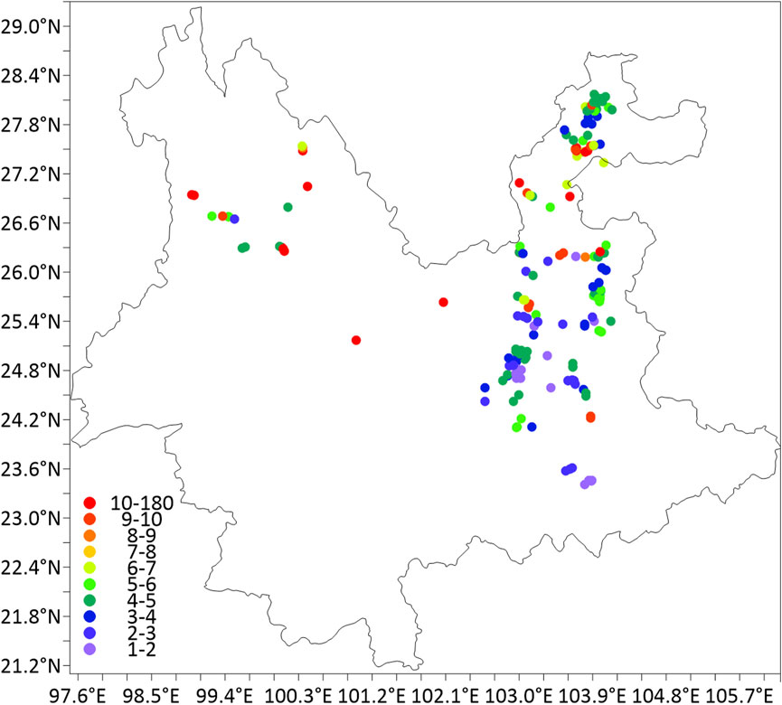
Figure 1. Distribution of observation points and their ice thickness of transmission lines in Yunnan Province.

2.2 Makkonen model

The Makkonen model (Makkonen et al., 2001) is the recommended icing model in the Atmospheric icing of structures (ISO 12494:2017). Based on atmospheric dynamics and thermodynamic principles, this model obtains icing thickness by calculating parameters such as air temperature, humidity and wind speed. The model also has high application value in icing simulation under freezing fog weather conditions. The model can be expressed as Eq. 1.

$\frac{dM}{dt}={\alpha }_1{\alpha }_2{\alpha }_{3}wAv(1)$

where M denotes the ice weight per unit length. α₁ indicates the collision efficiency, which is related to wind speed. a₂ represents the viscosity, which is nonlinearly correlated with wind speed (${\alpha }_2=1/v\left(v\ge 1\right)$; ${\alpha }_2=1\left(v<1\right)$). a₃ denotes the freezing rate related to temperature. w is the liquid water content per unit volume, which is considered to be a function of relative humidity. A represents the cross-sectional area of the icing body, which is considered constant for wires. V indicates the wind speed that is perpendicular to icing bodies. For macro meteorological factors, the air temperature, humidity and wind speed are the main factors affecting icing, and water bodies, windward/leeward slopes and mountain ridges can affect these meteorological factors. Based on this model, two simulation methods for icing thickness can be proposed.

2.3 Techniques for simulating wire icing thickness

2.3.1 A new method considering the weights of meteorological elements

Considering the relationships of icing thickness with air temperature, wind speed and water vapor in the Makkonen model, a regression model is established Eq. 2.

$Y=X\beta +\epsilon (2)$

where Y = [y₁, y₂, . . ., y_n]^T, and y_i (i = 1, 2, . . ., n) indciates the icing thickness at different moments (n). X denotes different variables, as shown in Eq. 3 (m is the number of variables).

$X=\left[\begin{array}{cccc}{x}_{11}& x_{12}& \cdots & x_{1m}\\ x_{21}& x_{22}& \cdots & x_{2m}\\ ⋮& ⋮& & ⋮\\ x_{n1}& x_{n2}& \cdots & x_{nm}\end{array}\right],\beta =\left[\begin{array}{c}{\beta }_1\\ {\beta }_2\\ ⋮\\ {\beta }_m\end{array}\right],\epsilon =\left[\begin{array}{c}{\epsilon }_1\\ {\epsilon }_2\\ ⋮\\ {\epsilon }_n\end{array}\right](3)$

where x_i,1 denotes the square of wind speed, x_i,2 the viscosity parameter (Eq. 4), x_i,3 air temperature and x_i,4 relative humidity. In order to further consider the impact of temperature on icing thickness, dew point temperature x_i,5 is introduced as an additional variable to simulate icing thickness.

$\left\{\begin{array}{c}{\alpha }_2=\frac{1}{v},v\ge 1\mathrm{m}/\mathrm{s}\\ {\alpha }_2=1,v<1\mathrm{m}/\mathrm{s}\end{array}\right.(4)$

In the solution process, coefficient β is obtained by the weighted least-squares (WLS) method (Yan et al., 2012), which can effectively eliminate the influence of outlier data. The specific formula is shown in Eq. 5. Note that the residual of the equation is set as Q.

$\begin{array}{l}\frac{\partial Q}{\partial \beta }=\frac{\partial {\sum }_i{\epsilon }_i^2}{\partial \beta }=\frac{\partial {\left(Y-\beta X\right)}^T\left(Y-\beta X\right)}{\partial \beta }\\ =-Y^{T}X+X^T{\beta }^{T}X=0\end{array}(5)$

Therefore, $\beta ={\left(X^{T}X\right)}^{-1}{X}^{T}Y,$ and $\epsilon =Y-\beta X$. As the weights of each moment are equal during the regression and the data is automatically collected by electronic instruments, there is a large uncertainty in the icing observations. It is necessary to consider the influence of outliers. Thus, the weighted least squares method is adopted to determine the weight at each moment, and the weight values are obtained by ${\omega }_i=1/{\epsilon }_i^2$. Eq. 5 can be rewritten as Eq. 6.

$\begin{array}{l}\frac{\partial Q}{\partial \beta }=\frac{\partial {\sum }_i{\omega }_i\epsilon {\prime }_i^2}{\partial \beta }=\frac{\partial {\left(Y-\beta X\right)}^T\left(Y-\beta X\right)}{\partial \beta }\\ =-Y^{T}WX+X^T{\beta }^{T}WX=0\end{array}(6)$

The coefficient β and covariance can be obtained by $\beta ={\left(X^{T}WX\right)}^{-1}{X}^{T}WY$ and ${\sigma }^2={\left(X^{T}WX\right)}^{-1}$, respectively. In the actual simulation process, the simulation data from the numerical model are adopted as the independent variable values, and thus, the obtained parameter β is regarded as consistent with the observation, which does not change in a short term. Hence, β can be iterated to the next step in the icing simulation. The results of the simulated icing thickness by this method are marked as P1.

2.3.2 Direct method based on the Makkonen model

In the Makkonen model, the product of parameters, such as viscosity, air temperature and relative humidity, is proportional to icing thickness. Therefore, a model is established, as presented in Eq. 7.

$y_{i,j}={\displaystyle \prod _{j=1}^m}{x}_{i,j}(7)$

The independent variable x_i,j is the same as that in Eq. 3. The result of the simulated icing thickness by this method is marked as P2.

2.3.3 AVT correction method

Based on the above icing thickness simulations, the AVT method (Zhang et al., 2019) is used to further eliminate deviations. The AVT method is considered to perform well in eliminating deviations. y_r and y_s represent the observed and simulated values, respectively, which are first de-trended separately by Eq. 8.

$\left\{\begin{array}{c}{y}_r^{\prime }=y_r-i\cdot h_r\\ y_s^{\prime }=y_r-i\cdot h_r\end{array}\right.(8)$

where h_r and h_s represent the trends of the observations and simulations, respectively, and the trends of the sequences are obtained by the least square method. y’_r and y’_s indicate the sequences after detrending. The averages and variances of the new sequences are further calculated and corrected by Eq. 9, and the corrected simulations $y_s^{″}$ have the same average and variance values as those of the observation sequence. In Eq. 9, a and σ denote the average and variance of corresponding sequences, respectively.

$y_s^{″}=\left(y_s^{\prime }-a_{y_s^{\prime }}+a_{y_r^{\prime }}\right)\frac{{\sigma }_{y_r^{\prime }}}{{\sigma }_{y^{\prime }s}}+i\cdot h_r(9)$

The observed values are unknown when the simulation is carried out. Therefore, these parameters can be determined by historical data and be iterated into new simulated results to achieve icing thickness simulations.

3 Results of icing thickness simulations

3.1 Simulations of icing thickness at single observation stations

The four-day icing process from January 8 to 11, 2021 is simulated by the two methods above according to different terrain patterns. In view of the simulations of different icing thicknesses grades, Figure 2 displays the icing simulations at an observation station (103.85°E, 27.89°N). The results indicate that the icing thickness values from January 8 to 11 are 3.12 mm, 3.41 mm, 3.42 mm, and 4.14 mm, respectively, suggesting that the icing thickness increases gradually. The icing thickness values of P1 are 2.90 mm, 3.62 mm, 3.62 mm, and 3.93 mm, with a mean absolute error (MAE) of 0.21 mm from the observations. However, the icing thickness values of P2 are 3.19 mm, 3.28 mm, 3.47 mm, and 4.15 mm, respectively, with a MAEs of 0.07 mm from the observations, and the Root Mean Square Error (RMSEs) are 0.21 and 0.08 respectively. Figure 3 shows the simulation results of icing at another observation station (103.69°E, 27.49°N). It can be seen that the icing thickness values at this station are similar to the results in Figure 2, but there are still simulation MAEs. From January 8 to 11, the observed icing thickness values were 3.39 mm, 4.32 mm, 4.40 mm, and 3.47 mm, respectively, the simulations of P1 are 3.96 mm, 3.37 mm, 4.62 mm, and 3.65 mm, respectively, and those of P2 are 4.22 mm, 3.64 mm, 3.27 mm, and 4.45 mm, respectively. The MAEs of the P1 and P2 simulations are 0.48 mm and 0.90 mm, respectively, and the RMSEs are 0.57 and 0.92 respectively. Therefore, the simulations of P1 are better than those of P2 when the thickness is between 0 mm and 5 mm.

Figure 2

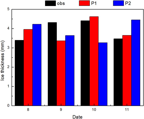
Figure 2. Observed and simulated ice thickness of the station (103.81°E, 27.81°N).

Figure 3

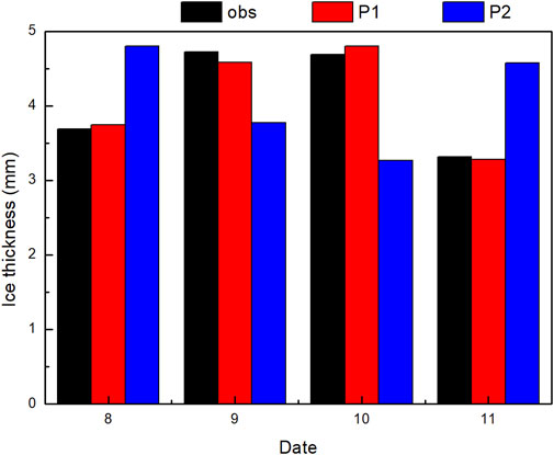
Figure 3. Same as Figure 2 but for the station (103.69°E, 27.49°N).

For the simulations of the 5–10 mm icing thickness, Figure 4 exhibits the simulation results at an observation station (103.84°E, 27.67°N). The observed icing thickness from January 8 to 11 was 4.40 mm, 5.76 mm, 5.72 mm and 4.45 mm, respectively, the simulations of P1 are 4.37 mm, 6.13 mm, 5.08 mm and 4.75 mm, respectively, and those of P2 are 5.75 mm, 4.35 mm, 4.51 mm, and 5.73 mm, respectively. The MAEs of the P1 and P2 simulations are 0.34 mm and 1.31 mm, respectively, and the RMSEs are 0.40 and 1.31 respectively. Figure 5 displays the results at the observation station located at 103.15°E, 24.12°N. The observed icing thickness values from January 8 to 11 are 4.17 mm, 4.46 mm, 6.12 mm, and 6.41 mm, respectively, the simulations of P1 are 4.32 mm, 4.35 mm, 5.88 mm and 6.60 mm, and those of P2 are 4.29 mm, 4.67 mm, 5.31 mm, and 6.88 mm. The MAEs of the P1 and P2 simulations from the observations are 0.17 mm and 0.41 mm, respectively, and the RMSEs are 0.18 and 0.48 respectively. It is illustrated that the simulations of P1 are better than those of P2 for the icing thickness between 5 mm and 10 mm.

Figure 4

Figure 4. Same as Figure 2 but for the station (103.84°E, 27.67°N).

Figure 5

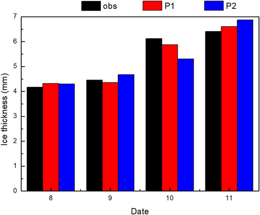
Figure 5. Same as Figure 2 but for the station (103.15°E, 24.12°N).

In terms of the icing thickness of 10–20 mm, the observed icing thickness values from January 8 to 11 at the observation station located at 103.70°E, 27.48°N (Figure 6) are 16.30 mm, 7.43 mm, 9.81 mm and 13.94 mm, respectively. The icing thickness values of P1 are 16.30 mm, 7.44 mm, 9.80 mm, and 13.95 mm, respectively, and those of P2 are 16.27 mm, 7.62 mm, 9.51 mm, and 14.08 mm, respectively. The simulation MAEs from the two methods from the observation are 0.01 mm (P1) and 0.16 mm (P2), and the RMSEs are 0.01 and 0.19 respectively. It can be concluded that both the MAE and RMSEs of the P1 simulations are also lower than that of the P2 simulations for the icing thickness between 10 mm and 20 mm.

Figure 6

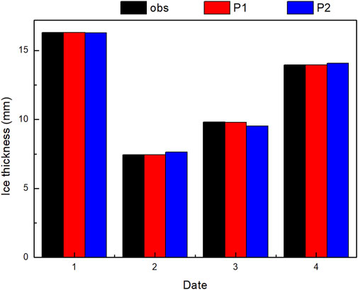
Figure 6. Same as Figure 2 but for the station (103.70°E, 27.48°N).

In the following, we further analyze the simulation MAEs from the two methods. Figure 7 presents the simulation results of icing thickness at an observation station (101.01°E, 27.17°N). The observed icing thickness values from January 8 to 11 at this station were 34.72 mm, 33.64 mm, 34.23 mm, and 32.57 mm, respectively, basically reaching the maximum icing thickness (40 mm) of this process. The icing thickness values of P1 are 34.37 mm, 34.19 mm, 34.20 mm, and 32.41 mm, respectively, and the results of P2 are 34.18 mm, 34.83 mm, 33.49 mm, and 32.67 mm, respectively, which are almost consistent with the observations. The simulation MAEs from the two methods are 0.28 mm (P1) and 0.64 mm (P2), and the RMSEs are 0.34 and 0.75 respectively, indicating the P1 simulations are still better in the case of icing thickness more than 20 mm.

Figure 7

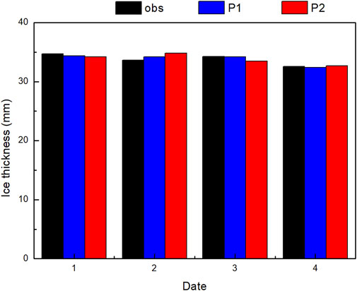
Figure 7. Same as Figure 2 but for the station (101.01°E, 27.17°N).

The icing thickness simulations at observation stations with different icing thickness grades Indicate that the simulation MAEs from the two methods are both approximately 2 mm, but the simulation MAE of P1 is smaller than that of P2. We simulate in bulk the icing data at 238 observation stations during this icing process, and analyze the simulation results of the two methods. The icing on January 8 is taken as an example (Figure 8). The results reveal that the two methods perform well in simulating the icing thicknesses at most observation stations (Figure 8A). In terms of the simulation MAEs (Figure 8B), the simulation MAEs of P1 are below 1 mm at most observation stations (84.46%), and only three observation station have simulation MAEs of more than 5 mm. The P2 simulations suggest that 59.66% of the observation stations show MAEs of less than 1 mm, 35.71% of the stations have MAEs between 1 mm and 2 mm, and there are 11 stations with MAEs of more than 5 mm. The MAE of icing thickness is 0.59 mm for P1 and 1.37 mm for P2, and the RMSEs are 1.79 and 4.10 respectively. A similar conclusion can be found in the icing case on January 9, 10, and 11 (figure omitted). Therefore, the simulation MAE of icing thickness from the new method considering the weights of meteorological elements is lower than that from the method that directly uses meteorological element products.

Figure 8

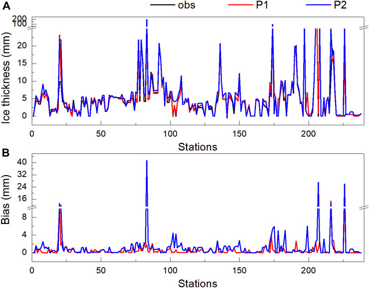
Figure 8. Ice thickness (A) and bias (B) at different stations.

3.2 Spatial differences of simulations

The spatial differences of the simulated icing thickness in this icing process indicate that the icing thickness simulated by the two methods is consistent with the observations at different stations, and the simulation MAEs are generally smaller (Figure 9). Specifically, the P1 simulation MAEs appear at the stations in northern and eastern Yunnan, and there are only 12 stations with MAEs of more than 1 mm. The P2 simulation MAEs mainly appear in the center of Yunnan, with 21 stations having MAEs of more than 1 mm and 3 stations showing MAEs of up to 5 mm.

Figure 9

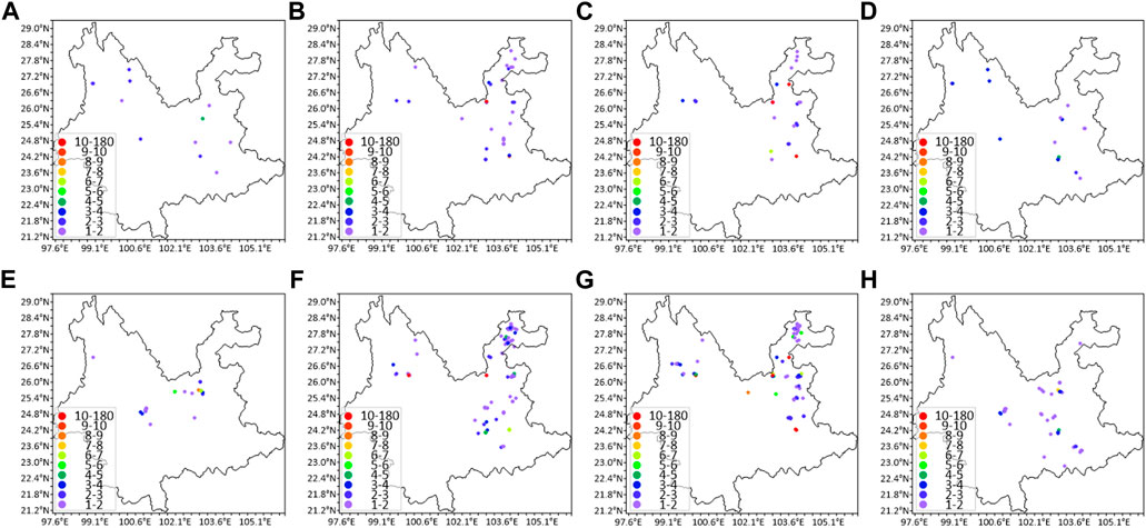
Figure 9. Ice thickness bias of different stations with P1 (A–D) and P2 (E–H) on January 8 (A,E), 9 (B,F),10 (C,G), and 11 (D,H).

On January 9, the overall icing thickness increases, especially in northeastern Yunnan, and the simulations are still close to the observations. However, with the increase of icing thickness, the number of stations with large MAEs also increases, and the MAEs of the P1 and P2 simulations are mainly concentrated in northeastern Yunnan, while the stations with larger P2 MAEs (1-2 mm) are more than those of larger P1 MAEs. That is, the stations with simulation MAEs of more than 1 mm are 31 for P1 and 69 for P2. Additionally, there are few stations with simulation MAEs exceeding 10 mm. On January 10, the number of stations with simulation MAEs also increases with icing thickness. However, the overall MAEs are still smaller, and the simulation MAEs at most stations are between 1 mm and 2 mm. The stations with larger P1 and P2 MAEs are still located in eastern Yunnan. Specifically, the number of stations with simulation MAEs above 1 mm is 25 for P1 and 78 for P2. On January 11, the icing process tended to end, the icing thickness decreased, and the MAEs of simulations gradually reduce. Moreover, the number of stations with large MAEs also decreases. Among them, the stations with larger P1 simulation MAEs are sporadically distributed in eastern and northern Yunnan, with 26 stations having simulation MAEs exceeding 1 mm. The stations with larger P2 simulation MAEs are mainly located in the central region of Yunnan, with 41 stations showing simulation MAEs exceeding 1 mm. Therefore, in terms of the number of stations with simulation MAEs, there are more stations with lower MAEs from P1 simulations.

4 Conclusion and discussion

According to the Makkonen model, an icing model recommended by Atmospheric icing of structures (ISO 12494:2017), a new ice thickness prediction model has been proposed to simulate icing thickness in Yunnan based on the simulation data from a mesoscale numerical model (Weather Research and Forecasting Model). The effectiveness of this method is verified by comparing the simulation results with observations. For the simulations of different icing thicknesses, the MAE (Table 1) from the proposed new model based on weighted coefficients is lower, which is about 2 mm (smaller than that from the traditional model). The spatial distribution of simulation MAEs also shows that this method is applicable in the vast majority of stations, and the simulation MAEs are lower.

Table 1

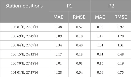
Table 1. MAEs and RMSEs of different observation stations.

It is worth noting that the simulation of icing thickness in this study relies on the model results and the icing thickness observations. The inherent MAEs in simulating meteorological elements, such as precipitation, wind speed, temperature, and pressure, can affect the prediction of ice cover thickness. The ice cover thickness observations used in this study are mainly obtained through sensor inversion, which often have certain MAEs. This introduces uncertainties when using observational data to correct the predicted results. By improving the quality of observational data, it can help improve the forecast results. Furthermore, sudden reductions in ice cover caused by human activities, animal activities, wildfires, and other factors are difficult to consider in the models, which also lead to inaccuracies in the predicted results. Therefore, in practical research on overhead wire icing, it is necessary to conduct comprehensive analysis and evaluation of these factors.

Data availability statement

The original contributions presented in the study are included in the article/Supplementary material, further inquiries can be directed to the corresponding authors.

Author contributions

FZ: Conceptualization, Writing–original draft, Writing–review and editing. XH: Conceptualization, Writing–review and editing. PY: Data curation, Formal Analysis, Investigation, Methodology, Writing–original draft, Writing–review and editing. XJ: Conceptualization, Supervision, Writing–review and editing. HP: Resources, Supervision, Writing–review and editing. YM: Supervision, Writing–review and editing. HG: Supervision, Writing–review and editing.

Funding

The author(s) declare financial support was received for the research, authorship, and/or publication of this article. This research has been supported jointly by the research on multi-time scale ice monitoring and prediction technology based on multi information fusion (YNKJXM20210174), the science and technology innovation Program of Hunan Province (2022GK2052), the key research and development program of Gansu (22YF7GA040).

Acknowledgments

We would like to express our gratitude to the Northwest Regional Center Numerical Weather Prediction team for providing technical support for the numerical simulation.

Conflict of interest

Authors FZ, HP, YM, and HG were employed by Yunnan Power Grid Co., Ltd. Author XH was employed by State Grid Hunan Electric Power Company Ltd.

The remaining authors declare that the research was conducted in the absence of any commercial or financial relationships that could be construed as a potential conflict of interest.

Publisher’s note

All claims expressed in this article are solely those of the authors and do not necessarily represent those of their affiliated organizations, or those of the publisher, the editors and the reviewers. Any product that may be evaluated in this article, or claim that may be made by its manufacturer, is not guaranteed or endorsed by the publisher.

References

Bretterklieber, T., Neumayer, M., Flatscher, M., Becke, A., and Brasseur, G. (2016). “Model based monitoring of ice accretion on overhead power lines,” in 2016 IEEE International Instrumentation and Measurement Technology Conference (I2MTC).IEEE, Taipei, Taiwan, 23-26 May 2016.

CrossRef Full Text | Google Scholar

Davalos, D., Chowdhury, J., and Hangan, H. (2023). Joint wind and ice hazard for transmission lines in mountainous terrain. J. Wind Eng. Industrial Aerodynamics J. Int. Assoc. Wind Eng. 232, 105276. doi:10.1016/j.jweia.2022.105276

CrossRef Full Text | Google Scholar

He, G. H., Hu, Q., Du, M. B., Zhang, Z., Wu, Z., Zhang, S. K., et al. (2021). Experimental research on the DC corona loss and audible noise characteristics of natural icing conductor. Proc. CSEE 41 (24), 9. doi:10.13334/j.0258-8013.pcsee.211257

CrossRef Full Text | Google Scholar

Huang, J. J., and Zhou, Y. (2015). The influence of topographic factors on wire icing in Hubei province. Torrential Rain Disaster 34 (3), 254–259.

Google Scholar

Janjua, Z. A. (2017). The influence of freezing and ambient temperature on the adhesion strength of ice. Cold Regions Sci. Technol. 140 (Aug), 14–19. doi:10.1016/j.coldregions.2017.05.001

CrossRef Full Text | Google Scholar

Ma, C., Cao, Y. H., and Chu, X. X. (2012). Ice shape prediction based on an improved thermodynamic model. Appl. Mech. Mater. 192, 63–67. doi:10.4028/www.scientific.net/AMM.192.63

CrossRef Full Text | Google Scholar

Makkonen, L. (1998). Modeling power line icing in freezing precipitation. Atmos. Res. 46 (1-2), 131–142. doi:10.1016/S0169-8095(97)00056-2

CrossRef Full Text | Google Scholar

Makkonen, L., Laakso, T., Marjaniemi, M., and Finstad, K. J. (2001). Modelling and prevention of ice accretion on wind turbines. Wind Eng. 25 (1), 3–21. doi:10.1260/0309524011495791

CrossRef Full Text | Google Scholar

Michal, T., and Bogdan, R. (2013). Analysis of frequency of occurrence of weather conditions favouring wet snow adhesion and accretion on overhead power lines in Poland. Cold regions Sci. Technol. 85, 102–108. doi:10.1016/j.coldregions.2012.08.007

CrossRef Full Text | Google Scholar

Ogretim, E., Huebsch, W. W., and Shinn, A. (2006). Aircraft ice accretion prediction based on neural networks. J. Aircr. 43 (1), 233–240. doi:10.2514/1.16241

CrossRef Full Text | Google Scholar

Savadjiev, K., and Farzaneh, M. (1998) Statistical analysis of two probabilistic models of ice accretion on overhead line conductors. California: International Society of Offshore and Polar Engineers.

Google Scholar

Savadjiev, K., and Farzaneh, M. (2004). Modeling of icing and ice shedding on overhead power lines based on statistical analysis of meteorological data. Power Deliv. IEEE Trans.19 (2), 715–721. doi:10.1109/TPWRD.2003.822527

CrossRef Full Text | Google Scholar

Wang, J. W. (2012). Ice thickness prediction model of transmission line based on improved particle swarm algorithm to optimize NRBF neural network. J. Electr. Power Sci. Technol. 27 (4), 76–80.

Google Scholar

Wu, X., Hu, X. X., Wang, B. B., and Chen, B. B. (2014). Mixed rime model of icing of wire in Guizhou area. J. Nat. Disasters 23 (3), 125–131. doi:10.13577/j.jnd.2014.0316

CrossRef Full Text | Google Scholar

Xu, F., Li, D., Gao, P., Zang, W., and Duan, Z. (2023). Numerical simulation of two-dimensional transmission line icing and analysis of factors that influence icing. J. Fluids Struct. 118, 103858. doi:10.1016/j.jfluidstructs.2023.103858

CrossRef Full Text | Google Scholar

Yan, P. C., Hou, W., Qian, Z. H., He Wen-Ping, , and Sun Jian-An, (2012). The analysis of the influence of globe SST anomalies on 500 hPa temperature field based on Bayesian. Acta Phys. Sin. 61 (13), 139202. doi:10.7498/aps.61.139202

CrossRef Full Text | Google Scholar

Yukino, T., and Yamaguchi, H. (2002). Analysis on influence of shape of snow/ice accretion on overhead transmission line conductor to its galloping phenomena. J. Cell. Biochem. doi:10.1260/175682509788913335

CrossRef Full Text | Google Scholar

Zhang, H., Zhang, S., Wang, Q., and Chai, H. (2021). The analysis of meteorological conditions for icing on UHV transmission lines in southeast guizhou in 2018. E3S Web Conf. 261, 01066. doi:10.1051/E3SCONF/202126101066

CrossRef Full Text | Google Scholar

Zhang, H. B., Wu, H. T., Hu, Q., Shu, L. C., and He, G. H. (2022). Influence of DC electric field intensity on conductor glaze icing and its corona loss. High. Volt. Appar. 58 (8), 0275–0279. doi:10.13296/j.1001

CrossRef Full Text | Google Scholar

Zhang, T. J., Yan, P. C., Li, Z. R., Wang, Y., and Li, Y. (2019). Bias-correction method for wind-speed forecasting. Meteorol. Z 28 (4), 293–304. doi:10.1127/metz/2019/0950

CrossRef Full Text | Google Scholar