Multi-device wind turbine power generation forecasting based on hidden feature embedding

In recent years, the global installed capacity of wind power has grown rapidly. Wind power forecasting, as a key technology in wind turbine systems, has received widespread attention and extensive research. However, existing studies typically focus on the power prediction of individual devices. In the context of multi-turbine scenarios, employing individual models for each device may introduce challenges, encompassing data dilution and a substantial number of model parameters in power generation forecasting tasks. In this paper, a single-model method suitable for multi-device wind power forecasting is proposed. Firstly, this method allocates multi-dimensional random vectors to each device. Then, it utilizes space embedding techniques to iteratively evolve the random vectors into representative vectors corresponding to each device. Finally, the temporal features are concatenated with the corresponding representative vectors and inputted into the model, enabling the single model to accomplish multi-device wind power forecasting task based on device discrimination. Experimental results demonstrate that our method not only solves the data dilution issue and significantly reduces the number of model parameters but also maintains better predictive performance. Future research could focus on using more interpretable space embedding techniques to observe representation vectors of wind turbine equipment and further explore their semantic features.

1 Introduction

Since the Industrial Revolution in the 18th century, with the advancement of technology and social progress, the demand for energy has grown rapidly (Wang et al., 2019). Conventional energy sources such as oil, coal, and natural gas not only have limited reserves but also contribute to environmental pollution and global warming (Wang et al., 2019). Wind energy, as a clean and widely distributed renewable energy, has gained global attention in recent years (Liu and Chen, 2019; Wang et al., 2021; Yang et al., 2021). However, the fluctuation of wind energy leads to the instability of power output in wind farms, which imposes additional burdens on energy storage devices and potentially affects the reliability of power supply (Parsons et al., 2004).

Incorporating efficient wind power forecasting methods into power control systems can effectively reduce operational costs and significantly enhance the reliability of wind power systems (Contaxis and Kabouris, 1991; Kariniotakis et al., 1996). Existing wind power forecasting methods mainly focus on individual devices. However, in practical applications, multiple wind turbines often operate in parallel within a wind power system. Assigning independent forecasting models to each device would result in two problems: firstly, dividing the dataset based on devices would lead to limited training data for each model, causing data dilution; secondly, each device having an independent model would result in a large number of total parameters, making accurate forecasting of wind turbine power generation increasingly challenging. In this paper, we propose a training method for prediction models applicable to multi-device scenarios, aiming to address the challenges of data dilution and excessive parameters.

2 Relevant work

The existing time series forecasting methods can be mainly divided into two categories: one consists of classical statistical methods with high interpretability and theoretical foundations, while the other category comprises more efficient methods based on artificial neural networks. The method proposed in this paper combines deep neural networks with space embedding technology from the field of natural language processing, aiming to effectively address the issue of multi-device wind turbine power generation forecasting.

2.1 Traditional wind power forecasting methods

The traditional wind power forecasting methods include physics-based models and statistic-based methods. The physics-based models play an crucial role in traditional forecasting methods, which consider meteorological factors (such as pressure, humidity, and temperature) from numerical weather prediction (NWP) and local topography for forecasting (Jung and Broadwater, 2014; Fang and Chiang, 2016; Hu et al., 2020). In terms of short-term forecasting capability, these methods generally perform moderately well, and their results are more suitable as a reference for long-term forecasting (Hu et al., 2020; Wang et al., 2021). The Autoregressive Integrated Moving Average (ARIMA) model, which is based on the theory of differencing, transforms non-stationary processes into stationary ones to address prediction problems (Ariyo et al., 2014). However, this method can only model individual attributes and fails to consider the correlations among multiple attributes at different time steps. In addition, ARIMA has high computational costs and is rarely applied to modeling and forecasting tasks involving long sequences.

2.2 Time-series forecasting methods based on deep learning

The commonly used wind power forecasting methods based on deep learning include two methods: Recurrent Neural Networks (RNN) and Transformer models. In comparison to the classical RNN model, its variants, such as Long Short-Term Memory (LSTM) (Hochreiter and Schmidhuber, 1997)and Gated Recurrent Unit (GRU) (Cho et al., 2014), are more prevalent. LSTM was proposed to address the problem of vanishing gradients caused by long sequence backpropagation. GRU, compared to LSTM, reduces the number of gate units and parameters, making it easier to train it to convergence. Additionally, it exhibits similar performance to LSTM in multiple tasks (Chung et al., 2014). Lai et al. advocated for forecasting models that encompass the impacts of both long-term patterns (such as day-night and season) and short-term patterns (like cloud fluctuations and wind direction). Building upon this concept, they introduced LSTNet, a variant of Convolutional Recurrent Neural Network (CRNN) (Lai et al., 2018). RNN possesses inherent capability in modeling time series data. However, the issue of gradient explosion has not been entirely solved yet. Moreover, their auto-regressive output mode not only extends the output time for long sequence forecasting tasks, but also increases training time due to challenges in parallel training.

The Transformer architecture was initially proposed for machine translation tasks (Vaswani et al., 2017). Although the Transformer model exhibits excellent performance in the field of NLP, its drawbacks are also evident: the model structure is complex, it has a large number of parameters, and it requires a relatively long time to produce outputs. Informer (Zhou et al., 2021) is a variant of the Transformer model designed for time series forecasting tasks. It incorporates the ProbSparse attention mechanism to reduce sampling time and introduces a generative decoder that can output the entire prediction sequence in a single step, significantly reducing the time complexity of the forecasting task. AutoFormer (Wu et al., 2021) introduces a novel attention mechanism called Auto-Correlation, which has stronger information aggregation capability, enabling it to achieve superior forecasting performance compared to variants such as Informer. However, the main advantage of the Transformer architecture lies in its multi-head attention mechanism, which exhibits permutation invariance. Even with the addition of positional encoding in the data, the application of attention mechanisms inevitably results in the loss of temporal information. In the field of natural language processing, semantics and word order are not entirely bound, but in the domain of time series forecasting, the output results are highly correlated with the temporal order. Zeng et al., 2023 have demonstrated that in some time series prediction tasks, a single-layer linear neural network outperforms Transformer-based networks and offers significant advantages.

2.3 Feature engineering

Feature engineering is the process of transforming raw data into features that better represent the essence of the problem. Effective feature engineering can consistently enhance the forecasting accuracy of the model. Two-dimensional Discrete Wavelet Transform (2D-DWT) and the 2D Fast Discrete Orthonormal Stockwell Transform (2D-FDOST) method are used to extract new effective dynamic features from dynamic electrical signals (Karasu and Sarac, 2019; Karasu and Saraç 2022). Compared to the Fourier transform, these methods exhibit stronger adaptability and noise resistance, allowing for localized analysis in different frequency domains and thereby capturing detailed features more effectively. However, these methods have a high computational complexity and are not suitable for scenarios requiring real-time processing. The Multi-Objective Grey Wolf Optimizer (MOGWO) is commonly used to extract a small set of useful features from a large volume of dynamic electrical signals, improving data quality and reducing computational overhead (Karasu and Saraç, 2020). The Grey Wolf algorithm has fewer parameters, is easy to implement, and requires less computational time, but the solutions found may not always be optimal. A feature selection method based on Sequential Floating Forward Selection (SFFS) has been used to reduce the historical operating data of lots of wind turbines in a wind farm environment to 660 effective features (Peng et al., 2021). This not only reduces the computational overhead of the forecasting model but also enhances its forecasting accuracy. However, the hyper-parameters of this algorithm are not adaptive, making it highly dependent on empirical expertise.

Methods for extracting dynamic features from historical power data are commonly used to assist neural network models in forecasting. However, the static features of wind turbine equipment have received less attention from researchers. Static factors, such as the type of wind turbine components, geographic environmental conditions, equipment layout, and equipment failure status, can also have a long-term impact on the power generation patterns of wind turbines, making them not entirely dependent on measurable internal conditions and weather factors.

Mikolov et al. (2013a), Mikolov et al. (2013b) both schemes infer the properties of words based on the distributional order of words in sentences. In natural language, there exist semantic and syntactic correlations between words, and deep learning models need to discover the semantic features hidden beneath the distributional order of words to accurately predict their sequence. However, apart from geographical location, there is no obvious distributional correlation among wind turbine devices. Therefore, CBOW and Skip-gram schemes are not suitable for the task of feature representation for wind turbines. The graph embedding technique (Grover and Leskovec, 2016) requires the model to predict the connectivity structure between nodes in the graph. Then, it utilizes gradient descent algorithm to infer high-dimensional vector representations of nodes or the entire graph. However, in a distributed wind farm, the geographical positions of wind turbines do not conform to the structure of a graph because there is no explicit connection between the nodes representing the wind turbines. Therefore, graph embedding techniques cannot be directly applied to the representation of wind turbine devices, nor can they directly uncover the hidden static features that influence the device’s own power generation patterns. Position Embedding (Vaswani et al., 2017), which is a manually specified method for encoding sequence order, utilizes a fixed calculation approach without neural networks or gradient descent algorithms. This method is applied in the position encoding of Transformer models. However, the hidden features of wind turbines are more complex than sequential order, and representation vectors calculated using manually specified algorithms based on device identifiers are unable to effectively reflect the characteristics of wind turbine devices.

Considering the complexity of static factors that influence wind turbine power generation patterns and the implicit correlations among turbines, this paper sets the task of training device representation vectors as power generation forecasting. To achieve this, the gradient descent algorithm is employed to evolve randomly initialized data into vectors that represent the static factors of the devices. This method directly uncovers hidden static factors that impact device power generation patterns. Different from traditional space embedding methods:

(1) Traditional space embedding methods are commonly used to generate generic representation vectors that are not specific to particular business scenarios. As a result, they fail to capture representation information in specific task scenarios. The proposed space embedding technique in this paper specifically addresses the task scenario of distributed wind turbine power forecasting, generating representation vectors that are exclusively applicable to this task scenario.

(2) In traditional space embedding methods, the tasks of generating entity representation vectors and the subsequent tasks of using these vectors often differ. The proposed space embedding method in this paper, however, aligns the task of generating vectors with the subsequent task, both of which is power generation forecasting.

2.4 Work presented in this paper

Classical statistical models, recurrent neural networks, and deep neural networks based on the Transformer architecture are all forecasting models designed for single devices. However, in multi-device scenarios, allocating independent prediction models for each device would result in data fragmentation, significantly reducing the available dataset for each model, while substantially increasing the total number of parameters. This paper presents an innovative method for wind power forecasting: instead of splitting the dataset according to devices or providing independent models for each device, a single model is trained to predict the power generation for each individual wind turbine device. The static characteristics of individual devices have an impact on the power generation patterns. However, a single prediction model cannot differentiate between different devices or take into account the differences in device operating patterns, leading to a loss in forecasting accuracy. To address this issue, this paper utilizes space embedding technology to infer the hidden features of each device and applies it to represent the wind turbines. The essence of space embedding technology is the same as that of neural networks, both of which are derived from causal effects and use gradient descent algorithms to calculate the static attributes that effectively affect the target task. Therefore, this article aims to propose a method that does not rely on expert knowledge and complex modeling processes to obtain the static properties of wind turbine equipment (including inherent equipment features and some long-term climate characteristics that do not change). During the power generation forecasting process, the representation vectors are concatenated with the temporal data and inputted into the neural network model. This approach enables the model to consider both the dynamic historical data and the inherent static characteristics of the devices. Experimental validation shows that the proposed method achieves a superior forecasting performance while reducing the parameter quantity to only 0.74% of the comparative method.

The main contributions of this paper are as follows:

(1) Proposed a method that utilizes the complete dataset for model training and employs a single model for wind power forecasting across multiple wind turbines. This method addresses the issue of data dilution and significantly reduces the number of model parameters.

(2) Introduced a space embedding technique specifically designed for wind turbines. This technique is used to represent the impact of hidden static features of the devices on power generation patterns, addressing the issue of predictive performance loss caused by an individual model’s inability to differentiate between devices.

(3) The experiments demonstrate that the single-model method using the complete dataset not only significantly reduces the number of parameters but also improves predictive performance. Building upon this foundation, the utilization of wind turbine embedding technology further enhances prediction accuracy. This paper verifies a positive correlation between the dimension of representation vectors and the accuracy of power generation forecasting. However, there is limited improvement in performance when the dimension becomes excessively large.

3 Theoretical background

3.1 Long Short-Term Memory

Long Short-Term Memory (LSTM) is a special type of Recurrent Neural Network (RNN). Compared to traditional RNN, LSTM alleviates the issues of vanishing and exploding gradients in modeling long sequences. When receiving input from the upper layers of the network, the LSTM layer needs to unfold itself horizontally to match the shape of the input data. The data flow mechanism of LSTM makes it naturally suitable for modeling sequential data, but also hinders parallel computation. The diagram below illustrates the data propagation and internal structure of LSTM during horizontal unfolding.

In Figure 1, the LSTM layer consists of multiple blocks, where each block shares the same parameters, and data propagation occurs strictly in linear order. Each LSTM block includes a forget gate $f_t$, an input gate $i_t$, and an output gate $o_t$. The forget gate $f_t$ controls whether historical information in the memory cell should be forgotten. The input gate $i_t$ determines whether the input data $X_t$ should be written into the memory cell. The output gate $o_t$ decides the extent to which information from the previous time step is transmitted to the next LSTM block. The formulas for these three gate units and the memory cell are as follows:

$f_t=\sigma \left(W_f\cdot \left[X_t,h_{t-1}\right]+b_f\right)(1)$

$i_t=\sigma \left(W_i\cdot \left[X_t,h_{t-1}\right]+b_i\right)(2)$

$o_t=\sigma \left(W_o\cdot \left[X_t,h_{t-1}\right]+b_o\right)(3)$

${\stackrel{\sim }{C}}_t=\mathit{tanh}\left(W_c\cdot \left[X_t,h_{t-1}\right]+b_c\right)(4)$

Figure 1

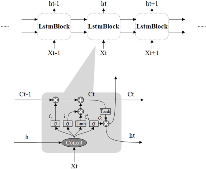
Figure 1. Illustration of LSTM layer structure.

In the formulas, $W$ and $b$ represent the learnable parameters and bias terms for each gate unit. $\sigma$ stands for applying the sigmoid activation function after performing matrix multiplication between the input data and the network parameter matrix. The formula for the sigmoid activation function is as follows:

$sigmod\left(x\right)=\frac{1}{1+e^{-x}}(5)$

The activation function will map the input data to a value between 0 and 1. The closer the value is to 0, the smaller the influence of the mapped data will be in the subsequent matrix multiplication. The formulas for the cell state $C_t$ and hidden state $h_t$ calculations are as follows:

$C_t=f_t\cdot C_{t-1}+i_t\bullet {\stackrel{\sim }{C}}_t(6)$

$h_t=o_t+\mathit{tanh}\left(C_t\right)(7)$

The derivative of $C_t$ with respect to $C_{t-1}$ is represented as $\frac{\partial C_t}{\partial C_{t-1}}=f_t+C_{t-1}\frac{\partial f_t}{\partial C_{t-1}}+\frac{\partial i_t}{\partial C_{t-1}}{\stackrel{\sim }{C}}_t{+i}_t\frac{\partial {\stackrel{\sim }{C}}_t}{\partial C_{t-1}}$, where $f_t$ falls between 0 and 1. Therefore, the internal structure of LSTM can effectively prevent the occurrence of gradient explosion or gradient vanishing.

3.2 Space embedding technology

Space embedding technology is a technique that computes the continuous vector representation of entities in a high-dimensional space. It originated from word embedding in the field of Natural Language Processing (NLP). Typically, space embedding technology evolves the vector representation based on the distribution phenomena or behavioral patterns of entities in specific tasks, evolving random data into high-dimensional vectors with representational capabilities. In the field of NLP, performing space embedding computation is an upstream task. This task is not specific to particular business scenario but rather aims to convert abstract natural language into a more easily processable data format. Conversely, downstream tasks are tailored to specific business scenarios and rely on the representations vector generated by upstream tasks. Figure 2 illustrates the relationship between upstream and downstream tasks.

Figure 2

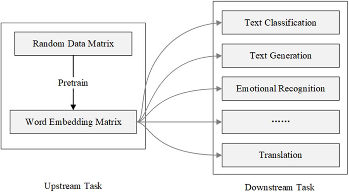
Figure 2. Diagram illustrating the association between upstream and downstream tasks.

Regarding the word embedding technology, predicting word distribution tasks are considered upstream tasks, while using evolved word vectors for tasks such as machine translation, sentiment analysis, or named entity recognition is referred to as downstream tasks. The distributional hypothesis proposed by Harris in 1954 serves as the theoretical foundation of word embedding technology. This hypothesis posits that words with similar contexts also have similar meanings and should correspond to similar high-dimensional continuous representation vectors (Harris, 1954). Word embedding technology derives high-dimensional continuous vector representations based on the phenomenon of word distribution. Typically, researchers train a deep neural network to predict word distributions and employ the gradient descent algorithm to update network parameters and word vector matrices simultaneously. After training the neural network until convergence, the high-dimensional vector representations corresponding to words have evolved from their random initial states to appropriate states. These representations can be used to describe the hidden features associated with each word. Representative models of this technology include word2vec, Elmo (Sarzynska-Wawer et al., 2021), Bert (Devlin et al., 2018).

After word embedding technology, embedding techniques have further developed into graph embedding for graph structures (Grover and Leskovec, 2016), position embedding for sequential order (Vaswani et al., 2017), and data embedding architecture known as data2vec for multi-modal data (Baevski et al., 2022), among other techniques or approaches.

It is crucial to recognize that power fluctuation patterns are influenced by both dynamic factors, such as changes in internal turbine states and meteorological conditions, and the static attributes of the turbine equipment. The design of turbine blades and the control strategy significantly affect energy capture and conversion efficiency, while the geographical and climatic context of the equipment directly impacts power generation fluctuations. Additionally, the static attributes of the turbine have a lasting impact on its power generation patterns, making its power output not entirely dependent on real-time internal and meteorological data. Even turbines of the same types may exhibit differences in their power generation patterns due to variations in environment, layout, and maintenance conditions.

However, characterizing the static features of turbines faces three challenges:

1. Although common SCADA datasets include a wealth of dynamic data from the operational phase, hey do not record details on common static features such as blade shape, wind adaptability, altitude, climate, and geographical environment.

2. It is challenging to analyze the correlation between a single static feature and power fluctuations, which limits our ability to discern and rank the relationship between static features and power fluctuations.

3. Analyzing the correlation between a single static feature and power fluctuations is challenging, which limits researchers’ ability to distinguish and rank the extent of correlation between static features and power fluctuations.

In the absence of effective features, researchers can predict the distribution of entities by training models to ensure the models capture the static hidden features of the entities. The Word2vec model infers the hidden semantic features of words based on the order of word distribution, and the graph embedding model node2vec infers the hidden features of nodes based on their connectivity structure in the graph. To overcome the challenges mentioned above and effectively capture the static features of turbine equipment, it is feasible to consider inferring potential static features based on the turbine power patterns.

We considered training models to infer hidden turbine features during the process of forecasting wind speed or direction. However, the static feature vectors generated in this way only reflect the climatic characteristics and do not represent the equipment characteristics (such as conversion efficiency, wind adaptability, or fault conditions). Constructing correlation graphs based on the similarity of power fluctuation patterns between turbines and using graph embedding techniques can also capture the static features of turbine nodes, though the static features obtained this way tend to represent inter-device correlations more. To comprehensively characterize the static factors affecting the equipment’s power pattern, we set both upstream and downstream tasks as the same, namely, the turbine power forecasting task. The representation vector generated based on this describes the static factors that affect the power fluctuation pattern. The vector semantics are not limited to climatic factors, equipment models, operational strategies, etc., but may also include other related factors that have not been researched but have a tangible correlation.

This paper presents an embedding technique that does not rely on entity distribution correlation. Specifically, when performing wind power forecasting tasks using neural networks, this paper utilizes the gradient descent algorithm to iteratively evolve randomly initialized vectors into high-dimensional representations of the wind turbine’s hidden static factors. Traditional space embedding techniques rely on predicting the distribution patterns of entities. However, in our method, we generate representation vectors by predicting the target attribute, i.e., Active power, directly. This method is not only applicable for generating representation vectors of entities without specific distribution phenomena, such as turbine generators, but also directly discovers hidden features that are highly correlated with the target attributes. The representation vectors generated by embedding technology are derived from longer segments of the training dataset, which allows them to encompass features from a wider time span. In contrast, the wind power forecasting task only accesses data from a limited number of historical time steps. The representation vectors provide additional evidence for the forecasting task. Subsequent experiments evaluated the impact of different dimensional representation vectors on the forecasting model, and verified the capability of embedding techniques to enhance the performance of the forecasting models.

4 Methodology

4.1 Task description

Wind power forecasting tasks fall into the category of time series forecasting tasks, which require models to predict future time steps based on historical time step data. Each time step corresponds to a sampling for factors such as turbine power, wind attributes, and internal device states. Typically, such tasks involve input data $\mathrm{X}\in {\mathrm{R}}^{\mathrm{K}\times \mathrm{T}}$, where K and T represent the number of historical time steps and the number of features per time step, respectively. After being processed by the forecasting model, the model’s output is denoted as $\mathrm{Y}\in {\mathrm{R}}^{\mathrm{N}\times \mathrm{T}}$, where N is the specified number of forecasting steps for the task. Specifically, in the scenario of single-property forecasting tasks, the model’s output is $\mathrm{Y}\in {\mathrm{R}}^{\mathrm{N}\times 1}$. In time series forecasting tasks, we aim for minimal discrepancy between the model’s predictions and actual measurement values.

In the proposed method, each wind turbine contains a vector ${\mathrm{h}}_{\mathrm{i}}\in {\mathrm{R}}^{\mathrm{M}}$ to represent its own characteristics, where M represents the number of attributes contained in the representation vector. The representation vector of the wind turbine will be concatenated with the dynamic temporal data and sent as part of the input data into the model. In this scenario, the input data of the model is $\mathrm{X}\in {\mathrm{R}}^{\mathrm{K}\times \left(\mathrm{T}+\mathrm{M}\right)}$, and the model output is $\mathrm{Y}\in {\mathrm{R}}^{\mathrm{N}\times 1}$.

4.2 Overview of method

In the proposed method of this paper, the wind power forecasting task is decomposed into two tasks: an upstream embedding task to infer the hidden features of wind turbines, and a downstream task to forecast power generation based on the hidden features.

The upstream and downstream tasks are not completely independent. As shown in Figure 3, the same data processing method and model architecture are used for model training in both the upstream and downstream tasks. The hidden static features generated by the upstream task are used as additional features, which will be concatenated with the historical time steps in the downstream task, and inputted into the LSTM model. In the proposed method, after the input data pass through the LSTM layer, Dropout layer, and linear projection layer, only the data representing future time steps is used as output, while the content representing historical time steps is discarded. The discarded portion does not contribute to the calculation of the loss function and does not have a positive effect on the optimization of the model parameters.

Figure 3

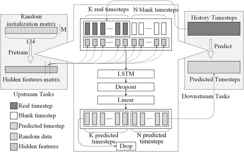
Figure 3. Overview of the method architecture.

4.2.1 Concatenation of blank time steps

In time series forecasting tasks, historical data is inputted into a neural network model, which then generates future data as output. In classical scenarios, researchers commonly utilize a sliding window approach to predict a limited number of time steps. Taking Figure 4 as an example, 4 previous time steps are used to forecast 1 subsequent time step, resulting in the generation of an entire time-series through multiple autoregressive iterations.

Figure 4

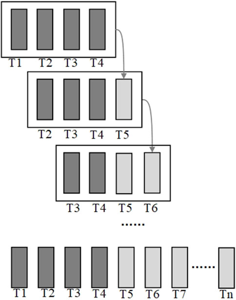
Figure 4. Diagram of autoregressive prediction method.

This paper argues that the method of the sliding window results in wastage of computational resources and time, as it requires inputting K historical time steps into the model for each prediction, and a long sequence needs multiple iterations to be fully generated. Therefore, this paper concatenates additional blank data with the historical time step to align the output format with the expected format. As shown in Figure 5, the prediction model needs to output data for N future time steps, with the number of blank time steps matching the desired output.

Figure 5

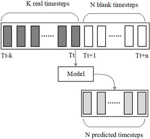
Figure 5. Diagram of the novel prediction method.

Due to the fact that LSTM can propagate data through the cell state $C_t$ and hidden state $h_t$ when unfolded, inputting blank time steps into the LSTM model does not cause interruption in information transmission.

4.2.2 Replication and concatenation of hidden features

The proposed hidden feature space embedding method aims to extract the hidden static features of the wind turbine devices thereby uncovering the latent factors that influence the operation patterns of the wind turbines.

As shown in Figure 6, in the process of pre-training, the hidden feature vector $h_i\in R^M$ corresponding to wind turbine i will be replicated K + N times. It is concatenated directly with historical time steps $X_i^h\in R^{K\times T}$ and blank time steps $X^b\in R^{N\times T}$, forming an input matrix ${Input}^{\left(K+N\right)\times \left(T+M\right)}$ with a shape of $\left(K+N\right)\times \left(T+M\right)$, which is then inputted into the LSTM model. This paper adopts the unique spatial dynamic wind power forecasting dataset, SDWPF (Zhou et al., 2022), provided by Longyuan Power Group Co., Ltd. This dataset contains a total of 134 wind turbines, so the hidden feature embedding matrix $H\in R^{134\times M}$ contains the representation vectors of 134 turbines. It is essential to ensure that the hidden feature vector $h_i$ and the historical time step $X_i^h$ are from the same turbine.

Figure 6

Figure 6. Replication and Concatenation process of hidden feature vectors.

The hidden features, as input data, participate in computation and obtain corresponding gradients through a backward propagation process. Subsequently, multiple rounds of iteration are performed using the gradient descent algorithm. The randomly initialized vectors gradually evolves into representation vectors that capture the hidden static features of the wind turbine devices. The algorithmic procedure is illustrated in Algorithm 1.

4.3 Evaluation metrics

This paper employs four performance evaluation metrics for forecasting models: Mean squared error (MSE), Mean Absolute Error (MAE), Pearson correlation coefficient (Corr), and coefficient of determination ($R^2$). The formulas for calculating these metrics are as follows:

$MSE=\frac{1}{\mathrm{n}}{\sum }_1^{\mathrm{n}}{\left(\widehat{{\mathrm{y}}_{\mathrm{i}}}-{\mathrm{y}}_{\mathrm{i}}\right)}^2(8)$

$MAE=\frac{1}{\mathrm{n}}{\sum }_1^{\mathrm{n}}\left|\widehat{{\mathrm{y}}_{\mathrm{i}}}-{\mathrm{y}}_{\mathrm{i}}\right|(9)$

$Corr=\frac{Cov\left(\widehat{\mathrm{y}},\mathrm{y}\right)}{\sqrt{Var\left(\widehat{\mathrm{y}}\right)\times Var\left(\mathrm{y}\right)}}=\frac{{\sum }_{\mathrm{i}}^{\mathrm{n}}(\widehat{{\mathrm{y}}_{\mathrm{i}}}-\overline{\widehat{\mathrm{y}}})\times \left({\mathrm{y}}_{\mathrm{i}}-\overline{\mathrm{y}}\right)}{\sqrt{{\sum }_1^{\mathrm{n}}{\left(\widehat{{\mathrm{y}}_{\mathrm{i}}}-\overline{\widehat{\mathrm{y}}}\right)}^2\times {\sum }_1^{\mathrm{n}}{\left({\mathrm{y}}_{\mathrm{i}}-\overline{\mathrm{y}}\right)}^2}}(10)$

$R^2=\frac{SSR}{SST}=\frac{{\sum }_1^{\mathrm{n}}{\left(\widehat{{\mathrm{y}}_{\mathrm{i}}}-\overline{\mathrm{y}}\right)}^2}{{\sum }_1^{\mathrm{n}}{\left({\mathrm{y}}_{\mathrm{i}}-\overline{\mathrm{y}}\right)}^2}(11)$

In the above equations, $\widehat{\mathrm{y}}$ represents the predicted values generated by the model, while $\mathrm{y}$ represents the measured values. The metrics of Mean Squared Error (MSE) and Mean Absolute Error (MAE) measure the discrepancy between the predicted values and the measured values, where smaller values indicate better performance.The Correlation (Corr) metric describes the degree of correlation between the predicted sequence and the actual sequence, with its value ranging from −1 to 1. A larger value indicates a stronger positive correlation, while a smaller value indicates a stronger negative correlation. The R-squared ($R^2$) metric quantifies the fitting degree of the predicted values to the actual values, with a value ranging between 0 and 1. Ideally, it should approach 1.

The forecasting model is prone to generating a straight line at the mean of the actual values as the prediction result, which exhibits a poor correlation with the actual values. Although the MSE and MAE metrics have small values in this case, the R-squared ($R^2$) metric approaches zero, indicating the model’s limited ability to capture volatility.

Furthermore, this paper introduces a custom comprehensive evaluation metric called Mean Standardized Score (MSS). It is calculated using the following formula:

$Score\left(x\right)=Corr\left(x\right)+R^2\left(x\right)-MSE\left(x\right)-MAE\left(x\right)(12)$

$MSS=Mean\left(\frac{Score\left(x\right)-Mean\left(Score\left(x\right),0\right)}{Std\left(Score\left(x\right),0\right)},1\right)(13)$

The calculation of the MSS metric consists of three steps:

(1) First, the original four evaluation metrics are summed according to the principle of adding positive gains and subtracting negative gains. This yields the total score of each model across all criteria.

(2) Then, the scores for each task are normalized. Due to the differences in task difficulty, the dimensions of the scores are inconsistent, resulting in tasks with higher scores having a greater impact on the final evaluation. Through the normalization operation, we ensure that the scores of each task have the same dimension, eliminating the influence of task difficulty on the final evaluation. Here, “$Mean\left(Score\left(x\right),0\right)$” and “$Std\left(Score\left(x\right),0\right)$"”mean taking the mean and standard deviation of the scores for different models under the same task.

(3) Finally, the scores of each task under the same model are averaged to determine the overall score of the model.

5 Experiment and analysis

5.1 Data preprocessing

This paper utilizes the unique spatial dynamic wind power forecasting dataset, SDWPF (Zhou et al., 2022), provided by Longyuan Power Group Co., Ltd. The dataset spans a period of 184 days and includes sampled data from 134 wind turbines. The SCADA system compiles the collected data at 10-min intervals, with each wind turbine accounting for 184 (days) × 24 (hours) × 6 (intervals), resulting in a total of 26,496 time steps. The entire dataset contains 26,496 × 134 (units), summing up to 3,550,464 time steps. Each time step is associated with 13 dynamic features, including data from internal features of the wind turbine equipment as well as climate-related data.

The content and format of the dataset are presented in the Table 1.

Table 1

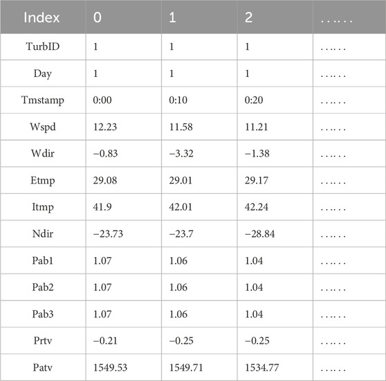
Table 1. Overview of dataset contents.

During the data preprocessing stage, the following steps were conducted on the dataset in this paper:

1. The feature of turbine ID was discarded. This paper employed space embedding technique to obtain a multi-dimensional vector representation of the hidden features of turbines. This method can provide richer turbine feature information for the model, whereas the turbine ID does not contain descriptive information about the static features of the device.

2. The feature of operating days was discarded. This feature is used to identify the sequential relationship between data. However, recurrent neural networks have the inherent ability to model time series data. Additionally, the data in the test set and validation set belong to future data, and this feature differs from the training set in terms of mean and variance, which can affect the model’s judgment. Therefore, this paper chooses to remove this feature.

3. Recoding the time feature. The format of this feature is “hour: minute,” and its content is not numerical, making it unsuitable for direct input into the model. In this paper, the timestamp was split to create two new dimensions. We hope the model can recognize the pattern of the relationship between power generation and the time variation within a day.

Figure 7 shows the data preprocessing process in a more intuitive way after preprocessing, the attributes of the dataset and their descriptions are shown in the Table 2.

Figure 7

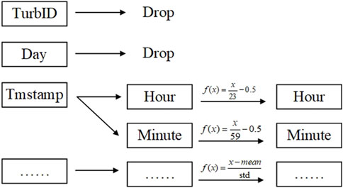
Figure 7. Diagram of data feature processing and normalization scheme.

Table 2

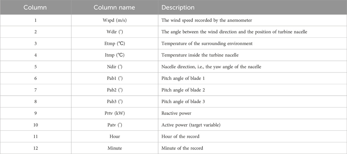
Table 2. Display of dataset features and descriptions.

This paper explores the correlation between multidimensional features and active power ($\text{Prtv}$), as shown in the heat map.

As depicted in Figure 8, a strong correlation is evident between active power (feature 10) and wind speed (feature 1), located at coordinates (1, 10). Additionally, there is an insignificant correlation between the active power (feature 10) and the temperature inside the turbine nacelle (feature 4), corresponding to coordinates (4, 10). Furthermore, the heatmap exhibits a strong negative correlation between the active power (feature 4) and the pitch angle of the three blades (feature 6, 7, and 8), corresponding to coordinates (7, 10), (7, 10) and (8, 10) respectively. The time feature (feature 10 and 11) shows few correlation with other features.

Figure 8

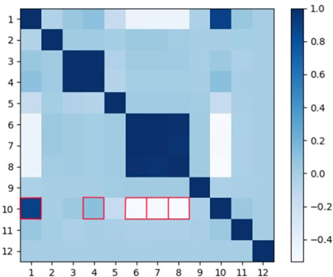
Figure 8. Heat map for attribute correlation analysis of the dataset.

5.2 Comparison between the improved method and traditional methods

In this research, 80% of the dataset is used as the training set, while the remaining 20% is allocated for the validation and test sets. Apart from the time feature, each dimension of the features is normalized using mean and standard deviation. The proposed method in this paper for multi-device power generation forecasting is not dependent on a specific neural network model, but can complement the improved methods of neural network models. Choosing an appropriate neural network model can improve the accuracy of power generation forecasting tasks in specific application scenarios. Conventional neural network models include but are not limited to Transformer and its variants, as well as recurrent neural network models such as LSTM or GRU. We adopts the LSTM as the experimental object and compares the performance difference between the traditional method and the single-model method that integrates space embedding technology. Table 3 displays the best results obtained from three experiments under the same conditions. Bold in the table is used to highlight the best results under the same experimental conditions, and the following table is the same.

Table 3

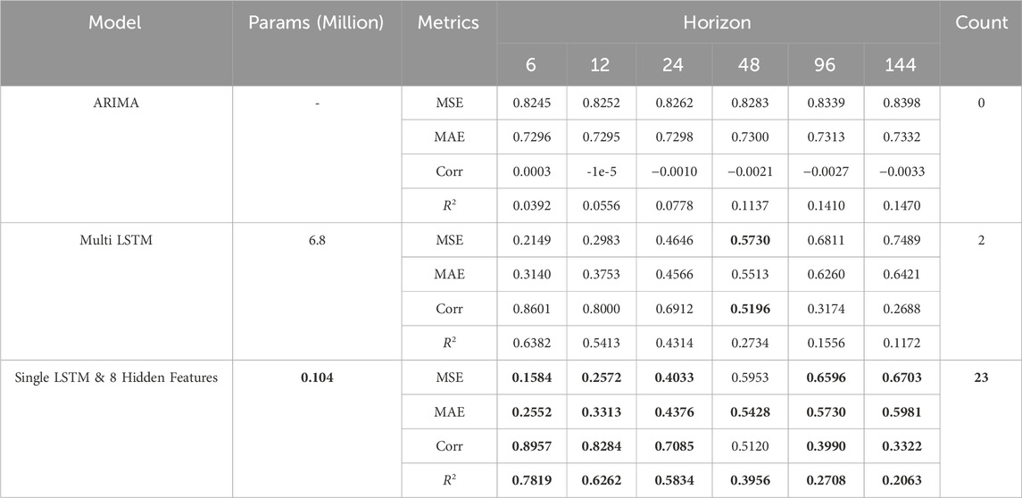
Table 3. Performance comparison between improved method and traditional method.

The “Multi LSTM” method in the table does not utilize the space embedding technique to obtain device representation vectors. Instead, it assigns a independent LSTM model to each turbine device for power generation forecasting. Since each device has an independent model, the dataset is also divided by devices. In the “Single LSTM & 8 Hidden Features” method, we use a single model and an undivided training set to forecasting the power generation of 134 turbine devices. At the same time, we introduce an 8-dimensional vector to represent the hidden static features of the turbine devices. The “ARIMA” scheme employs the classical statistical model ARIMA for power generation forecasting. The data in the table represents the average performance of all turbines’ predictions.

Based on the table results, it can be observed that the forecasting model using hidden features has fewer model parameters and demonstrates significant advantages across all four metrics. Particularly noteworthy is the 23.6% improvement in the MSE metric for ultra-short-term forecasting (1 h, 6 time steps). Compared to traditional approaches that merely input historical power data into neural network models, the method presented in this paper utilizes hidden features to represent the impact of wind turbine static attributes on their power generation patterns, enabling the forecasting model to make more accurate predictions based on the inherent properties of the equipment. Additionally, in traditional methods, since neural network models cannot distinguish which device the time series data originates from, separate forecasting models are assigned to each device. The dataset consists of 134 turbines, and the parameter size of the traditional method would reach 134 times that of the proposed method. This leads to wastage of computational resources without yielding significant performance improvements. However, the approach in this paper distinguishes devices based on hidden features which represent the differences between turbines, allowing the entire dataset to be used for model training. The augmentation of data also supports enhancements in forecasting accuracy. Additionally, due to the high randomness of the data, the performance of the statistic-based model ARIMA is not satisfactory.

We selected Wind Turbine NO. 1 and uses a 1-h ahead prediction to assess the short-term effectiveness of the forecasting model. By comparing Figure 9 and Figure 10, two advantages of the model trained with hidden features and the complete dataset can be observed:

• Higher accuracy: The results shown in Figure 10 demonstrate a stronger correlation between the orange line and the blue line. This observation aligns with the model’s superior performance over the traditional models in terms of correlation (Corr) and determination coefficient (R²) indicators.

• Higher certainty: Compared to Figure 9, the predicted values in Figure 10 exhibit smaller short-term fluctuations.

Figure 9

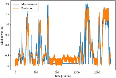
Figure 9. Forecasting performance of traditional method on wind turbine #1.

Figure 10

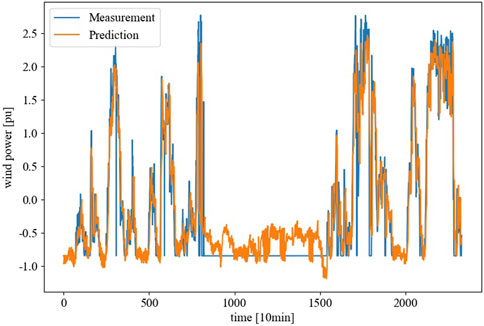
Figure 10. Forecasting performance of the Single Model method with 8 Hidden Features on wind turbine #1.

It should be noted that, the measured values from time step 700 to 1600 in the graph are displayed as 0, which is actually a result of data set incompleteness and filled with 0 instead of real measurements.

5.3 Performance evaluation on hidden feature dimensions

The above experiment compared the performance between the traditional method and the improved method that utilizes 8-dimensional hidden features. We will further examine the impact of additional dimensions of hidden features on the efficacy of the forecasting model in this research.

There are similarities in the power generation patterns among different wind turbines. Therefore, training the model using data from other wind turbines can enhance its emphasis on the conversion pattern between climate factors and power generation, thus reducing the risk of overfitting. The experiment demonstrates that even when the dimension of device representation vectors is 0, the forecasting performance of a single model is still superior to the traditional method of assigning independent models to each device. This implies that the negative impact caused by the inability of the model to differentiate between devices is smaller than the positive gain achieved through dataset augmentation. This phenomenon verifies the similarity in power generation patterns among wind turbine devices. In addition, the advantages of the forecasting model are more significant when the dimension of the device representation vector is higher. This phenomenon confirms the existence of differences in the power generation patterns among different devices. The information contained in the device representation vector provides additional features to the forecasting model, enabling more accurate predictions.

From Table 4, it can be observed that different dimensions of hidden features exhibit varying gain effects on the model. Among them, the 8-dimensional hidden features contribute the highest gain to the model. It is worth noting that Table 4 only explicitly compares the optimal performance under different conditions, without considering the negative impact of non-optimal attributes (non-bolded fields) on the performance of the method. Therefore, in order to compare the relative differences in model performance under different scenarios, we adopts the comprehensive scoring criterion MSS, aiming to comprehensively evaluate the methods.

Table 4

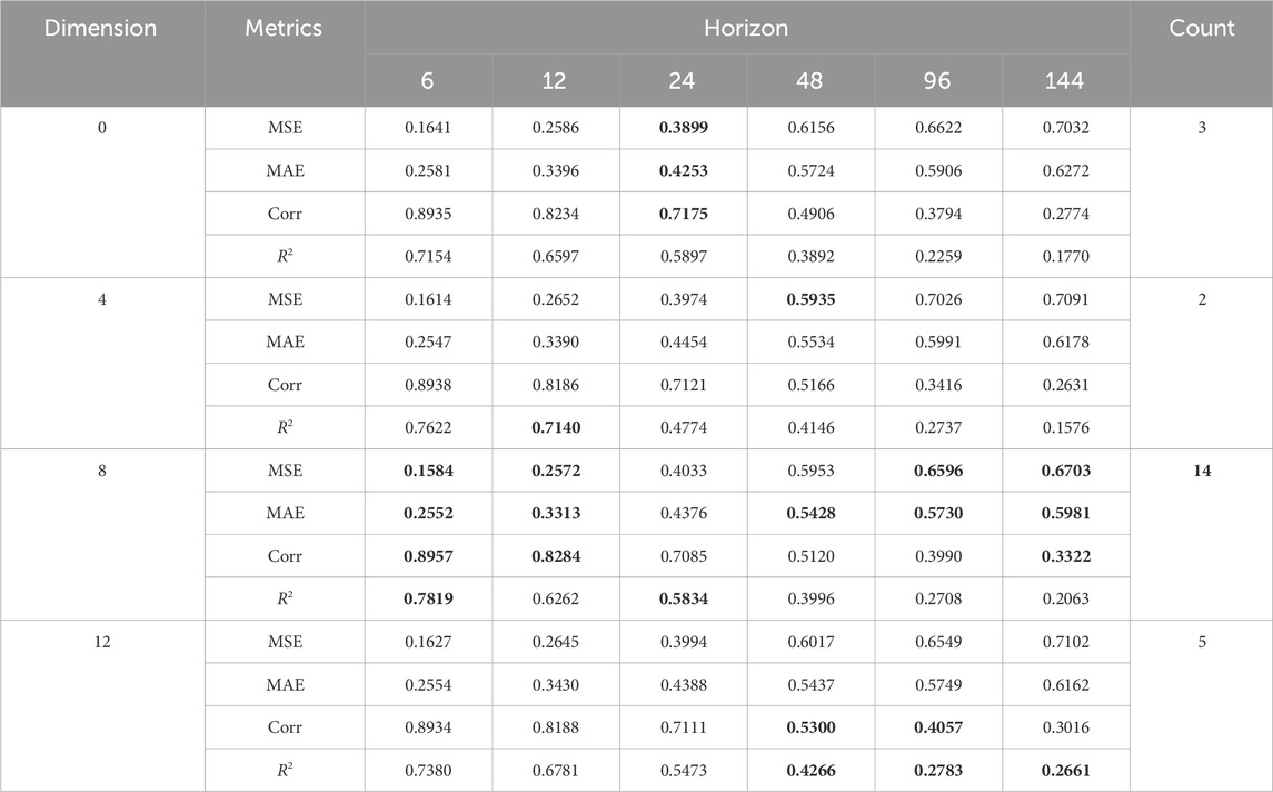
Table 4. Comparative results of models with different dimensions of hidden features on four criteria.

As shown in Table 5, it can be observed that although the 12-dimensional hidden feature model does not perform as well as the 8-dimensional model in terms of the number of optimal score quantity, its negative impact on non-optimal scores is less severe compared to the 8-dimensional hidden feature model. This results in a small difference in overall scores between the two models.

Table 5

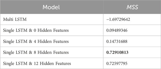
Table 5. Score table of models with different dimensions of hidden features under the MSS criterion.

The above performance differs from the space embedding task in natural language processing (NLP) tasks. In NLP tasks, word vectors usually have higher dimensions (512–1024 dimensions), while the dimensions of the hidden features of wind turbines are much lower than this range. 8-bit binary numbers can encode 256 entities, while the representation vectors generated by space embedding technique exhibit excellent representational capacity. Given that there are only 134 wind turbines, the number of hidden features should not differ significantly from 8 ([${\log }_2^{134}$] + 1). The gain of the model exhibited a turning point when the dimension of the representation vector was 8. This indicates that there is a certain degree of coupling between the static factors among wind turbines and their power generation patterns, and the number of independent influential factors is not substantial. The following figure demonstrates the iterative process of inferring the 12-dimensional representation vectors for wind turbines.

From Figure 11 and Figure 12, it can be observed that after being initialized with a normal distribution, some representation vectors exhibit the convergence of multiple features to the same point. This phenomenon confirms the existence of certain coupling between hidden static feature representations. Therefore, it can be concluded that a 12-dimensional hidden feature is not the most compact embedding representation for wind turbines. Excessive hidden features not only increase computational burden, but may also lead to overfitting of the prediction model. This paper argues that in this task scenario of distributed wind farm power generation forecasting, the number of hidden features should not be excessive. The results of the experiment demonstrate the effectiveness of static features in assisting forecasting, indicating that detailed features that affect the target task can be inferred to a certain extent without relying on specific expert knowledge and on-site detail modeling. However, the correspondence and representation effect between hidden features and real features in the on-site environment still need further research.

Figure 11

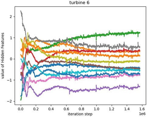
Figure 11. The 12-dimensional hidden features of Wind Turbine 6 converge to 8 points.

Figure 12

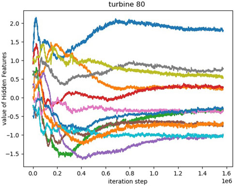
Figure 12. The 12-dimensional hidden features of Wind Turbine 80 converge to 7 points.

The hyperparameters used in the forecasting model for the experiment will be displayed in Table 6.

Table 6

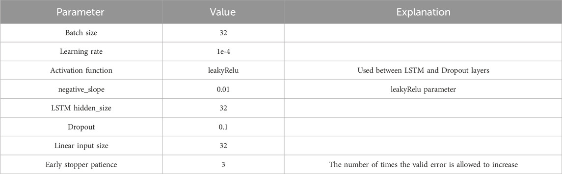
Table 6. Display of experimental parameter.

6 Conclusion

This paper investigates the problem of multi-device power generation forecasting in distributed power grid scenarios and proposes a forecasting method that combines space embedding techniques from the field of natural language processing. This method utilizes space embedding techniques to uncover hidden static features of each power generation device and uses these features as device identifiers. This allows a single model to distinguish between devices and accurately predict the power generation of multiple devices. The proposed method is independent of experimental models and does not rely on specific neural network architectures. It complements the improvements made in neural network algorithms. The experiments have shown that the proposed forecasting method, which integrates space embedding technology, not only significantly reduces the number of model parameters but also achieves higher prediction accuracy. The experimental results also indicate that the gain of representation vectors varies across different dimensions. The gain utility becomes less apparent, When the dimension of device representation vector is excessively large in the scenario described in this paper.

The proposed method in this paper focuses on using a single model to perform forecasting tasks for devices within the entire distributed power grid. However, there are several aspects that can be improved in the future:

(1) This paper confirms the compatibility of LSTM and space embedding technology. The subsequent investigation should involve considering the use of variants of the Transformer architecture to replace the classical LSTM model and verify the compatibility of space embedding technology with Transformer models in time series forecasting tasks.

(2) The representation vector of the wind turbine device is static data and does not vary with the time series, which is different from the temporal data. Currently, we concatenate the representation vector with the time steps data directly. In the future, we will consider using a more robust approach to integrate the device representation vector with the temporal data.

(3) The proposed prediction method integrates space embedding technology without relying on specific neural network architectures. Combining space embedding technology with models specific to the business scenario may lead to even better performance. In future work, we consider incorporating convolutional operations and attention mechanisms into the neural network to further enhance the accuracy of forecasting models.

Algorithm 1.Turbine Embedding.

Input: $H=\left\{h_1,h_2,\dots {,h}_{134}\right\}$, hidden features Matrix, includes hidden features of 134 turbines.

$X=\left\{x_1^1,x_2^1,\dots ,x_K^1,x_1^2,x_2^2,\dots ,x_K^2,\dots ,x_1^{134},x_2^{134},\dots ,x_K^{134}\right\}$, Historical data of 134 wind turbines, each sequence containing K time steps.

$Y=\left\{y_1^1,y_2^1,\dots ,y_N^1,y_1^2,y_2^2,\dots ,y_N^2,\dots ,y_1^{134},y_2^{134},\dots ,y_N^{134}\right\}$, Future data of 134 wind turbines, each sequence containing N time steps. $lr$, the learning rate

Output: hidden features Matrix $H$.

1 for epoch in range (1, 10), do:

2 for i in range (1, 134), do:

3 $input=\text{concat}\left(repeat\left(h^i,K,\mathit{dim}=0\right),X^i,\mathit{dim}=1\right)$

4 $\widehat{y^i}$ = LSTM $\left(input\right)$

5 loss = $\text{MSELoss}\left(\widehat{y^i},y^i\right)$

6 loss.backward

7 LSTM.parameters = LSTM.parameters $-$ LSTM.parameters.grads $\times lr$

8 $h_i$ = $h_i-$ $h_i$.grad $\times lr$

9 end for

10 end for

11 return H

Data availability statement

Publicly available datasets were analyzed in this study. This data can be found here: https://aistudio.baidu.com/aistudio/competition/detail/152/0/datasets.

Author contributions

JM: Conceptualization, Methodology, Writing–review and editing. KX: Software, Writing–original draft. DW: Data curation, Investigation, Writing–review and editing. YL: Investigation, Methodology, Writing–review and editing. JZ: Investigation, Writing–review and editing. YQ: Methodology, Resources, Writing–review and editing.

Funding

The author(s) declare that financial support was received for the research, authorship, and/or publication of this article. This research was funded by Key Technologies for Intelligent Monitoring and Analysis of Equipment Health Status of High of Science and Technology Innovation Team in College of Hunan Province, grant numbers 2023-233 (Xiang Jiao Tong), Natural Science Foundation of Hunan Province, grant numbers 2022JJ50002 and 2021JJ50049, Science and Technology Innovation Leading Plan Project of Hunan High Tech Industry, grant number 2021GK4008.

Acknowledgments

In my upcoming paper, I would like to take this opportunity to express my deepest gratitude to those individuals and institutions who have provided crucial support and assistance throughout my research journey. First and foremost, I want to sincerely thank my advisor. Thank you for providing valuable guidance, advice, and encouragement, helping me find the right direction in my research and offering unwavering support during times of difficulty. Furthermore, I would like to express my gratitude to the university for providing an excellent learning and research environment. Here, I had access to laboratory equipment and resources that were essential for my research work. Lastly, I would like to thank all my friends, classmates, and family members who have supported and assisted me throughout my research journey.

Conflict of interest

Authors DW and YL were employed by the CRRC Zhuzhou Electric Locomotive Research Institute Co., Ltd. Authors YQ were employed by the Guiyang Aluminum Magnesium Design and Research Institute Co., Ltd., Hunan Tianqiao Jiacheng Intelligent Technology Co., Ltd.

The remaining authors declare that the research was conducted in the absence of any commercial or financial relationships that could be construed as a potential conflict of interest.

Publisher’s note

All claims expressed in this article are solely those of the authors and do not necessarily represent those of their affiliated organizations, or those of the publisher, the editors and the reviewers. Any product that may be evaluated in this article, or claim that may be made by its manufacturer, is not guaranteed or endorsed by the publisher.

Supplementary material

The Supplementary Material for this article can be found online at: https://www.frontiersin.org/articles/10.3389/fenrg.2024.1346369/full#supplementary-material

References

Ariyo, A. A., Adewumi, A. O., and Ayo, C. K. (2014). “Stock price prediction using the ARIMA model,” in 2014 UKSim-AMSS 16th international conference on computer modelling and simulation, Cambridge, UK, 26-28 March 2014 (IEEE), 106–112.

CrossRef Full Text | Google Scholar

Baevski, A., Hsu, W.-N., Xu, Q., Babu, A., Gu, J., and Auli, M. (2022). “Data2vec: a general framework for self-supervised learning in speech, vision and language,” in International conference on machine learning (PMLR), 1298–1312.

Google Scholar

Cho, K., van Merriënboer, B., Bahdanau, D., and Bengio, Y. (2014). “On the properties of neural machine translation: encoder–decoder approaches,” in Proceedings of SSST-8, eighth workshop on syntax, semantics and structure in statistical translation, 103–111.

Google Scholar

Chung, J., Gulcehre, C., Cho, K. H., and Bengio, Y. (2014). Empirical evaluation of gated recurrent neural networks on sequence modeling. arXiv Prepr. arXiv:1412.3555.

Google Scholar

Contaxis, G. C., and Kabouris, J. (1991). Short term scheduling in a wind/diesel autonomous energy system. IEEE Trans. Power Syst. 6 (3), 1161–1167. doi:10.1109/59.119261

CrossRef Full Text | Google Scholar

Devlin, J., Chang, M.-W., Lee, K., and Toutanova, K. (2018). Bert: pre-training of deep bidirectional transformers for language understanding. arXiv Prepr. arXiv:1810.04805.

Google Scholar

Fang, S., and Chiang, H.-D. (2016). A high-accuracy wind power forecasting model. IEEE Trans. Power Syst. 32 (2), 1–1590. doi:10.1109/tpwrs.2016.2574700

CrossRef Full Text | Google Scholar

Grover, A., and Leskovec, J. (2016). “node2vec: scalable feature learning for networks,” in Proceedings of the 22nd ACM SIGKDD international conference on Knowledge discovery and data mining, 855–864.

Google Scholar

Harris, Z. S. (1954). Distributional structure. Word 10 (2-3), 146–162. doi:10.1080/00437956.1954.11659520

CrossRef Full Text | Google Scholar

Hochreiter, S., and Schmidhuber, J. (1997). Long short-term memory. Neural Comput. 9 (8), 1735–1780. doi:10.1162/neco.1997.9.8.1735

PubMed Abstract | CrossRef Full Text | Google Scholar

Hu, J., Heng, J., Wen, J., and Zhao, W. (2020). Deterministic and probabilistic wind speed forecasting with de-noising-reconstruction strategy and quantile regression based algorithm. Renew. Energy 162, 1208–1226. doi:10.1016/j.renene.2020.08.077

CrossRef Full Text | Google Scholar

Jung, J., and Broadwater, R. P. (2014). Current status and future advances for wind speed and power forecasting. Renew. Sustain. Energy Rev. 31, 762–777. doi:10.1016/j.rser.2013.12.054

CrossRef Full Text | Google Scholar

Karasu, S., and Sarac, Z. (2019). Investigation of power quality disturbances by using 2D discrete orthonormal S-transform, machine learning and multi-objective evolutionary algorithms. Swarm Evol. Comput. 44, 1060–1072. doi:10.1016/j.swevo.2018.11.002

CrossRef Full Text | Google Scholar

Karasu, S., and Saraç, Z. (2020). Classification of power quality disturbances by 2D-Riesz Transform, multi-objective grey wolf optimizer and machine learning methods. Digit. signal Process. 101, 102711. doi:10.1016/j.dsp.2020.102711

CrossRef Full Text | Google Scholar

Karasu, S., and Saraç, Z. (2022). The effects on classifier performance of 2D discrete wavelet transform analysis and whale optimization algorithm for recognition of power quality disturbances. Cognitive Syst. Res. 75, 1–15. doi:10.1016/j.cogsys.2022.05.001

CrossRef Full Text | Google Scholar

Kariniotakis, G. N., Stavrakakis, G. S., and Nogaret, E. F. (1996). Wind power forecasting using advanced neural networks models. IEEE Trans. Energy Convers. 11 (4), 762–767. doi:10.1109/60.556376

CrossRef Full Text | Google Scholar

Lai, G., Chang, W.-C., Yang, Y., and Liu, H. (2018). “Modeling long-and short-term temporal patterns with deep neural networks,” in The 41st international ACM SIGIR conference on research & development in information retrieval, 95–104.

CrossRef Full Text | Google Scholar

Liu, H., and Chen, C. (2019). Data processing strategies in wind energy forecasting models and applications: a comprehensive review. Appl. Energy 249, 392–408. doi:10.1016/j.apenergy.2019.04.188

CrossRef Full Text | Google Scholar

Mikolov, T., Chen, K., Corrado, G., and Dean, J. (2013a) Efficient estimation of word representations in vector space. arXiv preprint arXiv:1301.3781.

Google Scholar

Mikolov, T., Sutskever, I., Chen, K., Corrado, G. S., and Dean, J. (2013b). Distributed representations of words and phrases and their compositionality. Adv. neural Inf. Process. Syst. 26.

Google Scholar

Parsons, B., Milligan, M., Zavadil, B., Brooks, D., Kirby, B., Dragoon, K., et al. (2004). Grid impacts of wind power: a summary of recent studies in the United States. Wind Energy An Int. J. Prog. Appl. Wind Power Convers. Technol. 7 (2), 87–108. doi:10.1002/we.111

CrossRef Full Text | Google Scholar

Peng, X., Cheng, K., Lang, J., Zhang, Z., Cai, T., and Duan, S. (2021). Short-term wind power prediction for wind farm clusters based on SFFS feature selection and BLSTM deep learning. Energies 14 (7), 1894. doi:10.3390/en14071894

CrossRef Full Text | Google Scholar

Sarzynska-Wawer, J., Wawer, A., Pawlak, A., Szymanowska, J., Stefaniak, I., Jarkiewicz, M., et al. (2021). Detecting formal thought disorder by deep contextualized word representations. Psychiatry Res. 304, 114135. doi:10.1016/j.psychres.2021.114135

PubMed Abstract | CrossRef Full Text | Google Scholar

Vaswani, A., Shazeer, N., Parmar, N., Uszkoreit, J., Jones, L., Gomez, A. N., et al. (2017). Attention is all you need. Adv. neural Inf. Process. Syst. 30.

Google Scholar

Wang, Y., Hu, Q., Li, L., Foley, A. M., and Srinivasan, D. (2019). Approaches to wind power curve modeling: a review and discussion. Renew. Sustain. Energy Rev. 116, 109422. doi:10.1016/j.rser.2019.109422

CrossRef Full Text | Google Scholar

Wang, Y., Zou, R., Liu, F., Zhang, L., and Liu, Q. (2021). A review of wind speed and wind power forecasting with deep neural networks. Appl. Energy 304, 117766. doi:10.1016/j.apenergy.2021.117766

CrossRef Full Text | Google Scholar

Wu, H., Xu, J., Wang, J., and Long, M. (2021). Autoformer: decomposition transformers with auto-correlation for long-term series forecasting. Adv. Neural Inf. Process. Syst. 34, 22419–22430.

Google Scholar

Yang, J., Fang, L., Song, D., Su, M., Yang, X., Huang, L., et al. (2021). Review of control strategy of large horizontal-axis wind turbines yaw system. Wind Energy 24 (2), 97–115. doi:10.1002/we.2564

CrossRef Full Text | Google Scholar

Zeng, A., Chen, M., Zhang, L., and Xu, Q. (2023). Are transformers effective for time series forecasting? Proc. AAAI Conf. Artif. Intell. 37 (9), 11121–11128. doi:10.1609/aaai.v37i9.26317

CrossRef Full Text | Google Scholar

Zhou, H., Zhang, S., Peng, J., Zhang, S., Li, J., Xiong, H., et al. (2021). Informer: beyond efficient transformer for long sequence time-series forecasting. Proc. AAAI Conf. Artif. Intell. 35 (12), 11106–11115. doi:10.1609/aaai.v35i12.17325

CrossRef Full Text | Google Scholar

Zhou, J., Lu, X., Xiao, Y., Su, J., Lyu, J., Ma, Y., et al. (2022). Sdwpf: a dataset for spatial dynamic wind power forecasting challenge at kdd cup 2022. arXiv Prepr. arXiv:2208.04360.

Google Scholar