Short-term wind power forecasting based on dual attention mechanism and gated recurrent unit neural network

Accurate wind power forecasting is essential for both optimal grid scheduling and the massive absorption of wind power into the grid. However, the continuous changes in the contribution of various meteorological features to the forecasting of wind power output under different time or weather conditions, and the overlapping of wind power sequence cycles, make forecasting challenging. To address these problems, a short-term wind power forecasting model is established that integrates a gated recurrent unit (GRU) network with a dual attention mechanism (DAM). To compute the contributions of different features in real time, historical wind power data and meteorological information are first extracted using a feature attention mechanism (FAM). The feature sequences collected by the FAM are then used by the GRU network for preliminary forecasting. Subsequently, one-dimensional convolution employing several distinct convolution kernels is used to filter the GRU outputs. In addition, a multi-head time attention mechanism (MHTAM) is proposed and a Gaussian bias is introduced to assign different weights to different time steps of each modality. The final forecast results are produced by combining the outputs of the MHTAM. The results of the simulation experiment show that for 5-h, 10-h, and 20-h short-term wind power forecasting, the established DAM-GRU model performs better than comparative models on the basis of Root Mean Square Error (RMSE), Mean Absolute Error (MAE), R-squared (R²), Square sum error (SSE), Mean absolute percentile error (MAPE), and Relative root mean square error (RRMSE) index.

1 Introduction

The development and adoption of clean energy have a positive impact on protecting the environment, maintaining ecological balance, and reducing dependence on finite natural resources (Giebel and Kariniotakis 2017; Wang et al., 2021). Wind power, as a clean energy source, is steadily gaining prominence in the power grid. To meet the growing demand for electricity and achieve renewable energy goals, an increasing number of wind power projects worldwide are being connected to the electrical grid (Wang et al., 2022). However, the high unpredictability and volatility of wind energy can cause fluctuations in the frequency and voltage of the power system, which can be detrimental to the stability and quality of power. This simultaneously creates serious difficulties in scheduling and optimizing the grid (Duan et al., 2021).

The medium and long-term wind power forecasting is mainly to predict the annual and monthly power generation of wind farms to formulate power generation expectations and maintenance plans. Generally speaking, the results of short-term wind power forecasting have higher credibility than those of medium and long-term forecasting, so they can provide a good basis for grid scheduling, thus improving the ability of clean energy consumption. Therefore, improving the accuracy of wind power forecasting can provide an effective basis for grid scheduling, which is of great importance for the integration of large-scale wind power into the grid (Altan et al., 2021; Couto and Estanqueiro 2022).

There are two main approaches to wind power forecasting: statistical methods and methods based on physical principles. Physical methods use atmospheric science principles and meteorological data to estimate wind energy (Tian 2020). These physical methods are often employed for medium to long-term wind power forecasting, but short-term wind power forecasting heavily relies on conventional statistical approaches, such as exponential smoothing and time series analysis methods like the ARIMA model. These techniques generate short-term forecasts by analysing statistical features found in historical wind power data. However, wind power fluctuates a lot, and conventional models have a hard time explaining these intricate patterns (Liu et al., 2022). AI technologies, with deep learning as a prominent example, possess strong pattern recognition and data processing capabilities. Large-scale meteorological data and historical wind power generation data can be easily handled by them, improving the precision and dependability of power forecasting (Yang et al., 2021; Santhosh et al., 2018). Currently, ANN (Zhang et al., 2020), RNN Huang et al., 2021), and SVM (Tian and Chen, 2021a) are widely applied in time series forecasting tasks. Improved versions of RNN models are LSTM and GRU. They have achieved higher forecasting accuracy by addressing the issues of vanishing gradients and exploding gradients (Tian and Chen 2021b). LSTM is suitable for handling long-term dependencies but has a larger number of parameters, while GRU models are easier to train and achieve similar forecasting performance with fewer parameters (Liu et al., 2021; Saini et al., 2020). Therefore, in recent years, there has been an increasing amount of research on topics related to wind power forecasting using the GRU neural network as a basic model.

In Lin et al. (2021), gray correlation analysis was employed to select similar days. Subsequently, the data was inputted into a GRU model for wind power forecasting. This approach, compared to models like Autoregressive Integrated Moving Average (ARIMA), enhances forecasting accuracy. However, the method ignores the contribution of meteorological features in the historical data to the wind power output for the time period to be forecasted. In Xiao et al. (2023), the authors initially employ Weighted Principal Component Analysis (WPCA) with feature-weighted coefficients to reduce the dimensionality of wind power features. Subsequently, a GRU network optimized using the PSO algorithm is used for forecasting. The study considered the contribution of meteorological features to forecasts, but the contribution of individual meteorological features to forecasts varied over time and under different meteorological conditions. This shortcoming is remedied by Huang et al. (2023), the authors consider the spatiotemporal correlation among adjacent wind turbines. They initially reconstructed wind power data from 24 surrounding wind turbines and organized it into a three-dimensional matrix. They then use a combination of three-dimensional CNN and GRU models for forecasting. Pre-processing meteorological information and using historical power data to train the GRU network can improve forecasting accuracy by optimising the model to better capture the relationship between power and meteorology (Farah et al., 2022; Sun et al., 2023). In addition to the processing and extracting of meteorological features, it is equally important to consider sequence autocorrelation from the time series perspective. There are also related scholars conducting research in this area.

Attentional mechanisms have breathed new life into the field of natural language processing and have been widely used in time series forecasting tasks, where they have been shown to help forecasting models extract key information (Zhang et al. 2021). In Yang and Zhang (2021), the authors first use a Deep Attention Convolutional Recurrent Network (DACRN) to extract the features, then reconstruct the features using the developed auto-update memory module, then pattern cluster the feature reconstruction results using the K-shape clustering algorithm, and finally use the final prediction layer to predict the wind speed and experimentally validate the sophistication of the developed model. In Chi and Yang (2023), the authors utilized Wavelet Transform (WT) to eliminate noise from the sample data. Subsequently, they employed a combination of Temporal Attention Mechanism and Bidirectional Gated Recurrent Units (BiGRU) to model the data. Finally, the model’s performance was improved by utilizing a Time Convolutional Neural Network (TCN) to extract high-level temporal data. Trials have shown that this strategy improves forecasting accuracy. It is worth noting that the above two studies optimise and refine the baseline forecasting model in terms of meteorological features and time-series features respectively. However, the authors neglected the following three issues: first, the feature processing of both meteorological and time-series aspects are not well combined; second, the softmax function in the attention mechanism can achieve this effect well, but the original attention mechanism lacks the distinction of the relative position of the data in the time-series, which may require us to improve it when we use it for time-series feature extraction; Thirdly, it is possible that a single model could face some problems in extracting complex sequences directly, but data decomposition strategies were not considered for inclusion in the model.

Wind power data exhibits strong volatility, and achieving satisfactory accuracy through direct forecasting can be challenging. Therefore, decomposing wind power data and modeling forecasts separately for each component can effectively address this issue (Sun and Zhao 2020). In He and Wang (2021), the authors employ EEMD to decompose wind power time series into easily analyzable subseries. The LASSO-QRNN model is then used for forecasting. Finally, researchers use the Kernel Density Estimation (KDE) method for post-processing to obtain more accurate short-term wind power forecasting. In Abdoos (2016), the authors used Variable Modal Decomposition (VMD) to decompose the wind power series into different modes, and selected features using Gram-Schmidt Orthogonalisation (GSO), then used Extreme Learning Machine (ELM) to forecast the power of each mode, and finally superimposed the forecast results of each mode to obtain the final forecasting results. The data decomposition strategy can reduce the volatility of the time series and reduce the difficulty of forecasting for each model (Tian et al., 2020). However, in this strategy, the frequency of each modality is different, and it is difficult for the model to effectively integrate the meteorological features and better balance the importance of meteorological features and time series features.

Based on the above research results, this paper combines the advantages of the attention mechanism and the GRU network and improves them for the temporal attention mechanism, while using the idea of time series decomposition to better combine the two, and proposes a novel short-term wind power forecasting method which integrates the dual attention mechanism and GRU network. This method selects features in actual time by inputting power data and historical weather information into a feature attention layer. A GRU network is then used to make an initial forecasting. The output of the GRU network is then filtered using a number of one-dimensional convolutions with different kernel sizes. Ultimately, a MHTAM is used to assign weights to different time steps of each mode in a differential manner, and then the outputs are overlaid corresponding to the time steps to obtain the final forecast results.

In detail, the main contributions of the DAM-GRU model proposed in this paper to the study of short-term wind power forecasting are as follows:

1. Introduction of a feature attention mechanism that uses attention mechanisms to selectively extract historical meteorological or power features with higher contributions to the target forecasting time, while suppressing irrelevant features.

2. The model can better understand the characteristics and patterns of the wind power generation sequence by breaking it down and using one-dimensional convolution filtering with varying kernel sizes. This reduces the complexity of the sequence.

3. Introduction of a multi-head temporal attention mechanism to allocate varying weights to data at different time steps from multiple channels. This mechanism allows the model to simultaneously process information from different perspectives, rather than being confined to a single viewpoint, enabling the model to have a more comprehensive understanding of the temporal sequence structure.

The remaining portions of the paper are arranged as follows. The GRU model, the FAM, and the MHTAM are introduced in Section 2. The suggested integrated structure, the specific procedure, and the assessment metrics are all provided in Section 3. Comparing the merged model with other models and the model parameter settings, Section 4 examines the experimental outcomes. The study is finally summarized in Section 5.

2 Methods

2.1 Feature attention mechanism

Feature selection in wind power forecasting is a crucial step for improving model performance Meng et al. (2022). Correlation analysis methods like Pearson correlation coefficient can assist in selecting meteorological features to enhance forecasting accuracy (Liu et al., 2017). However, the Pearson correlation coefficient method overlooks the changing contributions of meteorological features to forecasts over time. The presence of the softmax function gives the attention mechanism excellent time selection capabilities. We introduce a feature attention mechanism to extract crucial features at different time points in real-time, while suppressing irrelevant features. This improves the adaptability and accuracy of the model. Figure 1 depicts the basic idea behind the feature attention method used in this investigation.

FIGURE 1

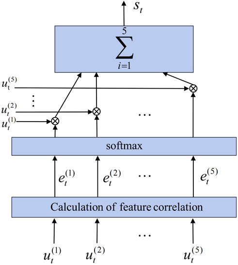
FIGURE 1. The feature attention mechanism schematic diagram.

The feature attention mechanism first calculates the similarity between wind power and meteorological features at the same time point to obtain attention scores for each element. Taking time step t as an example, the calculation of its attention score is shown in Eq. 1.

$e_t=v_e\tanh \left(w_e{u}_t+b_e\right)(1)$

where $u_t={[u_t^{(1)},u_t^{(2)},u_t^{(3)},u_t^{(4)},u_t^{(5)}]}^T$ represents the feature input vector at time step t, which includes five features for that moment: power, wind speed, wind direction, temperature, and air density; v_e and w_e is the weight. b_e is the bias term, and e_t encapsulates the attention score information for the five features at time step t.

Eq. 2 displays the probability distribution for the corresponding attention scores that are calculated using the softmax function.

${\beta }_t^m=\frac{\exp \left(e_t^m\right)}{{\displaystyle \sum _{i=1}^5}\exp \left(e_t^i\right)}(2)$

where ${\beta }_t^m$ contains the importance degree corresponding to the m-th feature at the moment t. Finally, based on this importance degree and the input features, the feature attention output s_t is obtained, as shown in Eq. 3.

$s_t={\displaystyle \sum _{i=1}^5}{\beta }_t^i\left(w_s{u}_t^i\right)(3)$

2.2 Multi-head temporal attention mechanism

The influence of historical data with different values and positions on the forecasting point varies. Attention mechanisms can capture these relationships. However, standard self-attention mechanisms lack control over the positional relationships in time series data. This results in assigning similar importance to historical data with different relative positions (Shih et al., 2019). To address these issues, this paper adopts the method proposed in reference (Yang et al., 2018) with some modifications. One of the modifications includes incorporating a Gaussian bias into the attention mechanism. This modification ensures that varying weights are assigned to data for each time steps. The Gaussian bias assigns different weights to attention scores for different positions, following a Gaussian distribution. The center position of the Gaussian function is automatically adjusted during parameter learning to focus on the region that is highly influenced by historical information for the current forecasting value.

The temporal attention mechanism is illustrated in Figure 2, with the input being the one-dimensional convolutional output sequence $h^{\prime }={[h_1^{\prime }.\cdot \cdot \cdot ,h_{t-1}^{\prime },h_t^{\prime }]}^T$. The calculation of attention scores in the temporal attention layer is described in Eq. 4.

$c=V_c\tanh \left(W_c{h}^{\prime }+b_c\right)(4)$

where V_c and W_c are weight matrices; b_c represents the bias term, and the attention score $c={[c_1,\cdots c_{t-1},c_t]}^T$.

FIGURE 2

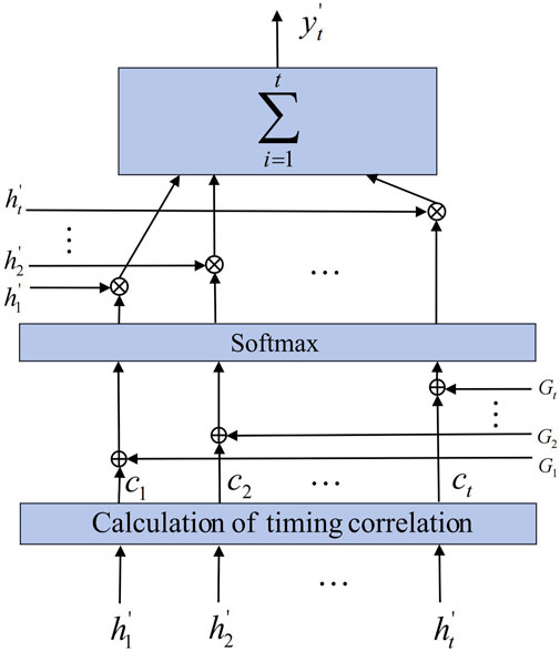
FIGURE 2. The temporal attention mechanism schematic diagram.

To achieve differential weight allocation across different time steps, Gaussian bias and attention scores are jointly input into the softmax function to compute attention probabilities α_t, as shown in Eq. 5.

${\alpha }_t=soft\max \left(w_{\alpha }{c}_t+G_t\right)(5)$

where w_α represents a weight factor; α_t represents the probability of the attention score at time step t, and G_t represents the Gaussian bias at time step t. G_t reflects the degree of closeness between the current moment and the central position moment, and its calculation method is as follows:

$G_t=-\frac{{\left(t-Q_t\right)}^2}{2{\sigma }^2}(6)$

$\left[\begin{array}{c}\hfill Q_t\hfill \\ \hfill D\hfill \end{array}\right]=I\cdot sigmoid\left(\left[\begin{array}{c}\hfill q_t\hfill \\ \hfill z\hfill \end{array}\right]\right)(7)$

$q_t=v_q\tanh \left(w_q{u}_t\right)(8)$

$\mathrm{z}=v_z\tanh \left(w_z\bar{K}\right)(9)$

where Q_t represents the center position at time step t, and its value is ultimately determined based on the parameter u_t, which is learned based on the value of t; σ is set to $\frac{D}{2}$, where D is the window size for this mode, each mode has a separate window to define its window range, with a larger value indicating a longer sequence related to the current time step; I is a real number that ranges from 0 to the input sequence’s length; v_q, v_z, w_q and w_z are weight coefficients, and z is the scalar factor for selecting the window for this mode; $\bar{K}$ in the original reference represents the key-value relationship between semantics. Here, it is set to be the same as the kernel size k of the one-dimensional convolution. The underlying idea is that if a mode has a larger convolution kernel, its window will be larger. This allows different sequences to have different linear characteristics, aiding the model in capturing trend components of time series data.

Eq. 10 illustrates how the output of the temporal attention layer is finally calculated based on the probability α_i of the temporal attention scores.

${y_t}^{\prime }={{\displaystyle \sum _{i=1}}}^t{\alpha }_i\left(w_{y^{\prime }}{h_i}^{\prime }\right)(10)$

A single temporal attention mechanism is responsible for capturing the temporal weights of a single channel, while the multi-head temporal attention mechanism simply combines them. Applying one-dimensional convolutions with multiple diverse kernels to filter the GRU network’s output is necessary to guarantee that each temporal attention mechanism can extract distinct patterns of temporal information. When the length of the convolution kernel is k, the convolution formula is as shown in Eq. 11.

${h_i}^{\prime }=\mathrm{R}\mathrm{e}Lu\left({\displaystyle \sum _{l\in M_H}}{w}_l{h}_{il}+b_l\right)(11)$

where $h_i^{\prime }$ represents the ith element of the feature map; $\mathrm{R}\mathrm{e}Lu\left(\cdot \right)$ represents the activation function. M_H represents the spatial extent of the convolution kernel; w_l is the corresponding weight; h_il represents the lth element in the input data with i as the center; b_l is the bias of the convolution kernel. After the convolution output undergoes feature extraction through the temporal attention mechanism, the results are summed up with step-wise weighting, as shown in Eq. 12.

$p_t={\displaystyle \sum _{i=1}^H}{w}_p{y}_{i\left(t\right)}^{\prime }(12)$

where the projected output of the model at time step t is denoted by p_t; The output of the ith temporal attention head at time step t is denoted by $y_{i(t)}^{\prime }$; w_p corresponds to the weight associated with it. H represents the total number of attention heads.

Figure 3 shows the details of the implementation of the multi-head temporal attention mechanism.

FIGURE 3

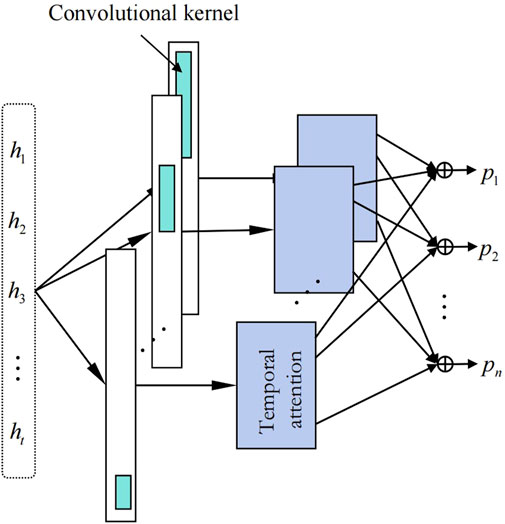
FIGURE 3. Architecture of multi-head temporal attention mechanism.

2.3 GRU

Compared to the complex LSTM, the GRU has a simpler structure and higher computational efficiency. In this paper, the GRU network is chosen as the main component to construct the model. The feature selection and forgetting functions of GRU are implemented by only reset gates and update gates. GRU is relatively more efficient in terms of computational efficiency and number of parameters due to its simple structure. The update gate determines how much of the past information is retained, and the parameter values of the update gate are learned through training thus allowing the GRU unit to dynamically capture long-term dependencies in the sequence. The reset gate controls the inflow of historical information into the candidate hidden state and thus determines whether to disregard past information (van Heerden et al., 2022). Its internal structure is depicted in Figure 4.

FIGURE 4

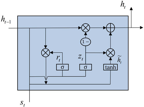
FIGURE 4. Internal structure of GRU unit.

Taking moment t as an example, the inputs to the gated loop unit are s_t and the hidden state h_t−1 from the previous moment. Inputs are processed to calculate the outputs of the update gate and reset gate, which are represented by Eqs 13, 14.

$r_t=\sigma \left(w_{sr}{s}_t+w_{hr}{h}_{t-1}\right)(13)$

$z_t=\sigma \left(w_{sz}{s}_t+w_{hz}{h}_{t-1}\right)(14)$

where w_sr, w_hr, w_szand w_hz represent weight terms; r_t is the output of the reset gate, and z_t is the output of the update gate; σ represents the sigmoid function.

The reset gate is used to determine the significance of the output from the previous time step. It combines this information with the current input to calculate the current hidden state, as shown in Eq. 15.

${\tilde{h}}_t=\tanh \left(w_{sh}{s}_t+w_{hh}{h}_{t-1}\otimes r_t\right)(15)$

where w_sh and w_hh represent the weight terms for the importance at time step t and time step t − 1, respectively. ${\tilde{h}}_t$ signifies the hidden state at time step t, and ⊗ denotes the Hadamard product.

Eq. 16 is the final calculation used to determine the output of the GRU at the current time.

$h_t={\tilde{h}}_t\otimes z_t+h_{t-1}\otimes \left(1-z_t\right)(16)$

According to Eq. 16, when the update gate output z_t approaches 0, the output of the GRU unit is mainly determined by the output of the previous time step. Conversely, when z_t approaches 1, it is primarily determined by the hidden state of the current time step (Liu et al., 2023).

3 Model design

3.1 DAM-GRU model calculation process

Wind power is subject to weather conditions that are highly random and volatile. In order to decompose and predict wind power generation while considering climate features comprehensively and avoiding situations where historical information is insufficiently learned, such as forecasting lag, we establish a forecasting model that combines feature-based temporal dual attention mechanisms with GRU networks. The complete structure of the model is depicted in Figure 5.

FIGURE 5

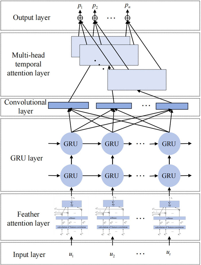
FIGURE 5. DAM-GRU model architecture.

The DAM-GRU model-based short-term wind power forecasting procedure is as follows:

1) Normalize the power, wind speed, temperature, and air density features using Eq. 17.

$u_{\mathit{norm}}=\frac{u-u_{\min }}{u_{\max }-u_{\min }}(17)$

where u_norm represents the normalized result. The text represents the values of the four mentioned feature sequences. The maximum and minimum values in the raw data are denoted by u_max and u_min, respectively. Normalize the wind direction feature using Eq. 18.

$u_{\mathit{norm}}^{\left(3\right)}=\sin \left(u^{\left(3\right)}\right)(18)$

where $u_{\mathit{norm}}^{(3)}$ represents the normalized result of the wind direction feature, and u⁽³⁾ represents the wind direction feature sequence.

2) The FAM assigns different weights to meteorological features based on different weather conditions. This allows it to dynamically extract key features in real time, improving the forecasting process.

3) Making initial predictions using a two-layer GRU model based on the extracted features.

4) One-dimensional convolutional models with H convolutional kernels of different sizes are used to apply convolutional filtering operations to the initial forecasting results of the GRU model. This is done to extract the timing patterns of wind power for different time series and reduce the complexity of individual timings.

5) In order to avoid forecasting lag, assign temporal feature weights to the H distinct periodic patterns independently using a multi-head temporal attention technique.

6) Combine the predictions of each sub-sequence by performing a weighted summation. Reverse the normalization process to obtain the final forecast result.

3.2 Evaluation metrics

In order to statistically assess the accuracy of the wind power forecasting model, we compare RMSE, MAE, R² SSE, MAPE, and RRMSE using the following formulas:

$RMSE=\sqrt{\frac{1}{n}{\displaystyle \sum _{i=1}^n}{\left({\widehat{p}}_i-p_i\right)}^2}(19)$

$MAE=\frac{1}{n}{\displaystyle \sum _{i=1}^n}\left|{\widehat{p}}_i-p_i\right|(20)$

$R^2=1-\frac{{\displaystyle \sum _{i=1}^n}{\left({\widehat{p}}_i-p_i\right)}^2}{{\displaystyle \sum _{i=1}^n}{\left({\widehat{p}}_i-\bar{p}\right)}^2}(21)$

$SSE={\displaystyle \sum _{i=1}^n}{\left({\widehat{p}}_i-p_i\right)}^2(22)$

$MAPE=\frac{1}{n}{\displaystyle \sum _{i=1}^n}\left|\frac{{\widehat{p}}_i-p_i}{{\widehat{p}}_i}\right|\times 100\%(23)$

$RRMSE=\sqrt{\frac{1}{n}{\displaystyle \sum _{i=1}^n}{\left(\frac{{\widehat{p}}_i-p_i}{{\widehat{p}}_i}\right)}^2}(24)$

where $\bar{p}$ denotes the average value of the actual value sequence, n represents the number of forecast steps, p_i and ${\widehat{p}}_i$ represent the predicted and actual values for the ith sample point, respectively. Smaller RMSE, MAE SSE, MAPE, and RRMSE indicate better model performance, while an R² closer to 1 indicates higher accuracy (Tian 2021; Tian et al. 2021).

4 Case study

The experiment was conducted on a hardware platform consisting of a GeForce GTX 1050Ti GPU with 2 × 8 GB DDR4 memory. The programming language used was Python 3.7, and the model was constructed using the TensorFlow 2.1 deep learning framework.

In order to validate the performance of the proposed model, power and meteorological data collected from a wind farm located in Inner Mongolia, China, were used for the experiments. The dataset covers the time range from January 1 to 30 June 2020, and the data is sampled every 15 min, resulting in a total of 17,568 data points. Where 14,000 data points are allocated for the training set, 250 data points are allocated for validation, and 3,318 data points are allocated for testing. The installed capacity of the wind farm is 100 MW. Each epoch consists of 80 batches, with a training batch size of 100 and a learning rate of 0.001. The training phase utilizes the Adam optimizer.

4.1 Model parameter configuration

The forecasting model employs feature sequences of length 30 steps as input, meaning that wind power for future n time steps is predicted using the previous 30 steps of features. The number of FAM heads in the model is equal to the number of input time steps. A double-layer GRU network is employed for the preliminary forecasting of wind power, with each layer containing 64 GRU units. The choice of attention heads is crucial, and in this case, parameter tuning experiments are conducted under 20 steps forecasting horizon. The number of attention heads, denoted as H, is tested with values of 2, 3, 4, 5, and 6, and the fluctuation of errors under different attention head numbers is shown in Table 1. The minimum error is achieved when H is set to 4. The convolutional kernels corresponding to the 4 attention heads have sizes of 3 × 1, 5 × 1, 7 × 1, and 9 × 1, with a stride of 1, the edge padding strategy is set to “same”, and the activation function is set to “ReLU”. The number of time steps in which the model outputs its forecasts is the number of output time steps for each TAM.

TABLE 1

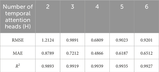
TABLE 1. Influence of the number of temporal attention heads on error.

4.2 Validation of model effectiveness

In this paper, three core components of the DAM-GRU model are the FAM, the GRU network, and the MHTAM. In order to emphasize the diversity of each time feature, a Gaussian bias is added to the multi-head time attention module. To evaluate the influence of each component of the DAM-GRU model on forecasting performance, this section compares the model with other models that use the same dataset and GRU network parameters. The DAM-GRU models compared include the GRU model, GRU-TAM model, FAM-GRU model, and GRU-MHTAM model. The GRU-TAM model combines a temporal attention mechanism with a single head within the GRU network. To ensure a fair comparison in the experiments, a 3 × 1 convolutional kernel is used to filter the initial forecasts made by the GRU. The FAM-GRU model combines the FAM with the GRU network, while the GRU-MHTAM model combines the GRU network with the multi-head temporal attention mechanism. The forecasting horizons are categorized into three levels: 20 steps (5-h), 40 steps (10-h), and 80 steps (20-h). Correspondingly, the lengths of the historical sequences are 30 steps, 60 steps, and 120 steps. This means that the model uses historical input sequences of 30, 60, and 120 steps to forecast power values for 20, 40, and 80 steps into the future, respectively.

Figure 6 show the comparison of forecast curves and box plots for five models at forecasting durations of 5-h, 10-h, and 20-h. All three sets of forecast curves show that the single GRU forecast model has a significant lag. This lag is attributed to its limited ability to efficiently extract highly correlated meteorological and time series features. The inclusion of the FAM and single-head temporal attention mechanism results in varying degrees of improvement, as evident in three box plots. The incorporation of the MHTAM leads to a significant enhancement in model performance. The proposed model in this paper demonstrates excellent feature extraction capabilities, making it adaptable to the rapid fluctuations in wind power. Overall, it demonstrates a significant decrease in lag and improved alignment with the observed values compared to the other models. Overall, the errors in model forecasts increase rapidly with increasing forecast length, and certain models have varying degrees; of outlier forecasts. This implies that the models require additional features to account for variations in the meteorological data as the forecast time horizon increases. The forecasting process becomes more complex and challenging due to various external factors that can impact the output of wind power.

FIGURE 6

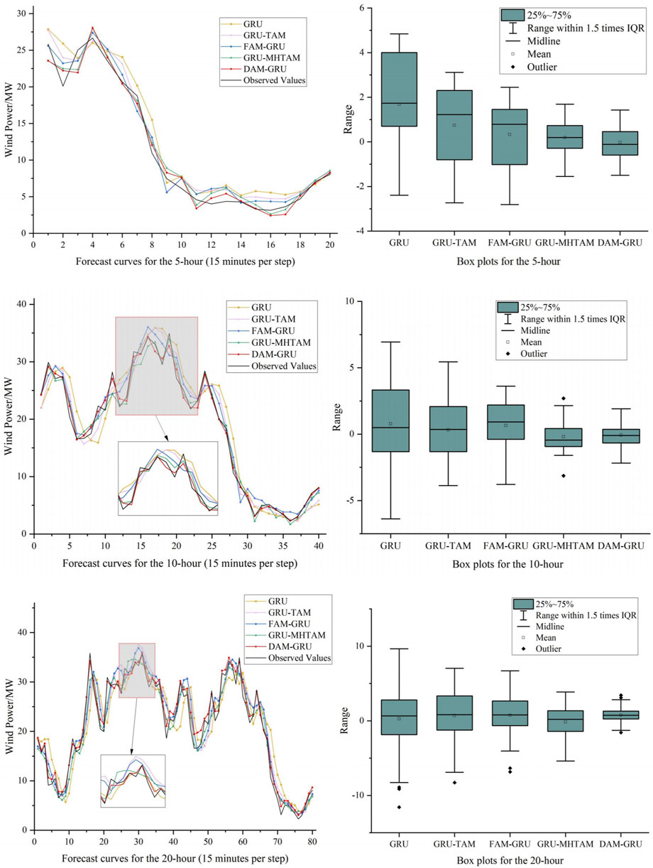
FIGURE 6. 5-h, 10-h and 20-h forecast curves and box plots for 5 models including GRU, GRU-TAM, FAM-GRU, GRU-MHTAM, and DAM-GRU.

Table 2 shows a comparison of the predictive performance for different attention mechanisms at 5-h, 10-h, and 20-h. From the table, it can be observed that the forecasting errors of all models increase rapidly as the forecasting steps increase, while the goodness-of-fit indicator, the coefficient of determination (R²), decreases. This suggests that longer-term sequences exhibit weaker regularity and higher complexity, making it more challenging for models to extract features. The performance of the forecasting model can be improved by incorporating temporal and feature attention mechanisms. The model can more easily adjust to the intricacy of wind power sequences because of these attention mechanisms, which provide it the flexibility to focus on various attributes and time steps. Taking the 20-h forecast results as an example, the GRU-TAM model reduced the RMSE, MAE, SSE, MAPE, and RRMSE error metrics by 26.3%, 18.5%, 45.6%, 19.1%, and 24.6% respectively, and increased the R² by 3.4% compared to the GRU model. On the other hand, the FAM-GRU model reduced the RMSE, MAE, SSE, MAPE, and RRMSE errors metrics by 35.8%, 32.4%, 58.8%, 25.2%, and 33.8% respectively, and increased the R² by 4.3% compared to the GRU model. This demonstrates the necessity of adding attention mechanisms to help the GRU model extract features and temporal information. The GRU-MHTAM model, compared to the GRU-TAM model, reduces the RMSE, MAE, SSE, MAPE, and RRMSE error metrics by 53.0%, 56.4%, 78.9%, 53.7%, and 52.8% respectively, and increases R² by 3.0%. This suggests that the MHTAM can be effective in dealing with time series features. In this experiment, the parts of the DAM-GRU model are split and tested for comparison, which proves the validity of the model design method from two perspectives: feature and time series, and demonstrates that the DAM-GRU model has good forecasting performance.

TABLE 2

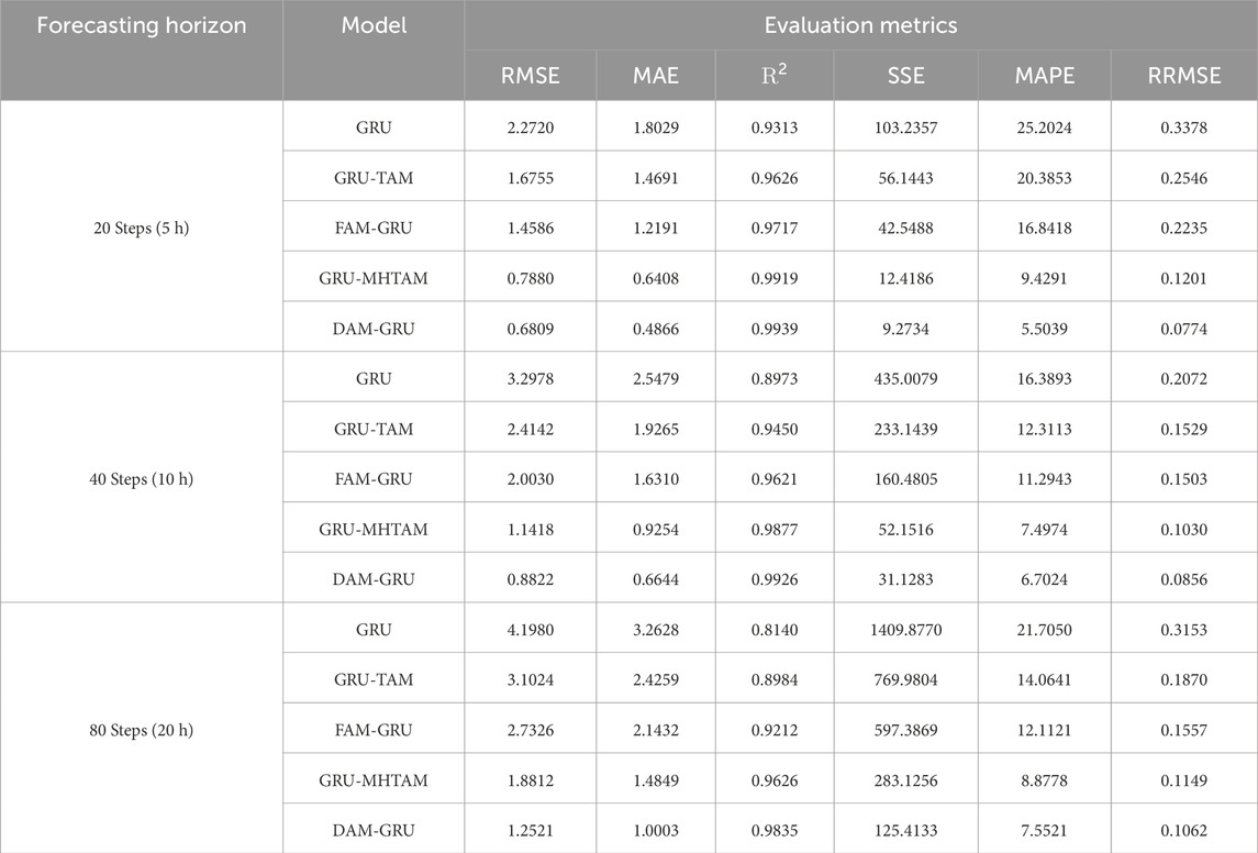
TABLE 2. Comparison of predictive performance with different attention mechanisms.

Table 3 shows a comparison of the time required for training and forecasting for the five models. The time required for training and prediction is not strictly increasing or decreasing due to complex factors such as GPU performance and initial parameters within the model, but generally shows some degree of regularity. From the table, it can be seen that the sum of training time for FAM-GRU and GRU-MHTAM is similar to the sum of training time for GRU and DAM-GRU, and the forecast time has the same pattern, which is consistent with the number of parameters of the model. As the number of forecast steps increases, the time required for training and forecasting may also increase, due to the fact that an increase in the number of forecast steps corresponds to an increase in the number of units in the input layer of the model.

TABLE 3

TABLE 3. Comparison of training time and forecasting time with different attention mechanisms.

4.3 Forecasting performance tests

In order to test whether the proposed DAM-GRU model has advanced prediction performance, we select CNN-GRU (Gao et al., 2023), VMD-CNN-GRU (Zhao et al. 2023), and MTTFA-GRU (Liu and Zhou, 2024) under the same data set algorithms as comparison models for the experiment. Among them, the number of input features of CNN-GRU and MTTFA-LSTM models is 5, the VMD-CNN-GRU model uses VMD decomposition to decompose the wind speed into four submodules, and then combines them with the wind power series using the CNN-GRU model to predict. To ensure the fairness of the experiments, the training batch size and iteration number of the comparison models are the same as the models in this paper, using the same settings.

At forecast horizons of 5 hours, 10 hours, and 20 hours, Figure 7 compare the suggested DAM-GRU model with three models. Box plots and forecast curves are compared in the figures. We find that the DAM-GRU model forecasts values that are quite similar to the observations. It demonstrates excellent predictive performance even during rapid changes in wind power over a short time frame. When combined with the accuracy metrics presented in Table 4, the DAM-GRU model outperforms the comparative models for forecasting horizons of 5 h, 10 h, and 20 h. Specifically, for a forecasting horizon of 5 h, the proposed model reduces RMSE, MAE, SSE, MAPE, and RRMSE forecasting errors by 6.0%, 18.9%, 11.7%, 20.6%, and 11.3% respectively, and increased the R² by 0.8% compared to the MTTFA-LSTM model. For 10 and 20 h, The DAM-GRU model also outperforms the MTTFA-LSTM model to varying degrees. The DAM-GRU model’s performance is also superior to that of the CNN-GRU and VMD-CNN-GRU models. The validity of the DAM-GRU model was further confirmed.

FIGURE 7

FIGURE 7. 5-h, 10-h and 20-h forecast curves and box plots for 4 models including CNN-GRU, VMD-CNN-GRU, MTTFA-LSTM, and DAM-GRU.

TABLE 4

TABLE 4. Comparison of multi-stage forecasting errors with other classic GRU-based models.

To compare the training and forecasting time of the proposed DAM-GRU model with other mainstream and advanced GRU-based models. Table 5 shows that the proposed DAM-GRU model has a slight increase in training time and forecasting time compared to CNN-GRU, VMD-CNN-GRU, and MTTFA-LSTM models, but considering its obvious improvement in forecasting performance and that the time spent in actual online training is much less than the length of forecasting for each training, it can meet the technical requirements in practical applications.

TABLE 5

TABLE 5. Comparison of multi-stage training time and forecasting time with other classic GRU-based models.

4.4 Comparison with traditional models

In order to fully understand the difference between the forecasting performance of the DAM-GRU model and the traditional models, this section selects 4 traditional models including ARMA, RF, SVM and BP, and conducts comparative experiments using the same experimental strategy as in Section 4.3. The autocorrelation order of ARMA is set to 25, and the moving average order is set to 3. The number of decision trees of RF model is 80, and the minimum number of leaves is 5. SVM adopts Radical Basis Function (RBF) as the kernel function to build a regression model with multidimensional variables. The BP neural network has 6 units in the input layer, which are used to input 5 features and the forecasting results from the previous step, the hidden layer has 15 units for high dimensional mapping, and the output layer has one node for multi-step cyclic forecasting. Figure 8 shows a comparison of the forecast curves and box plots for each model when forecasting 20, 40 and 80 steps.

FIGURE 8

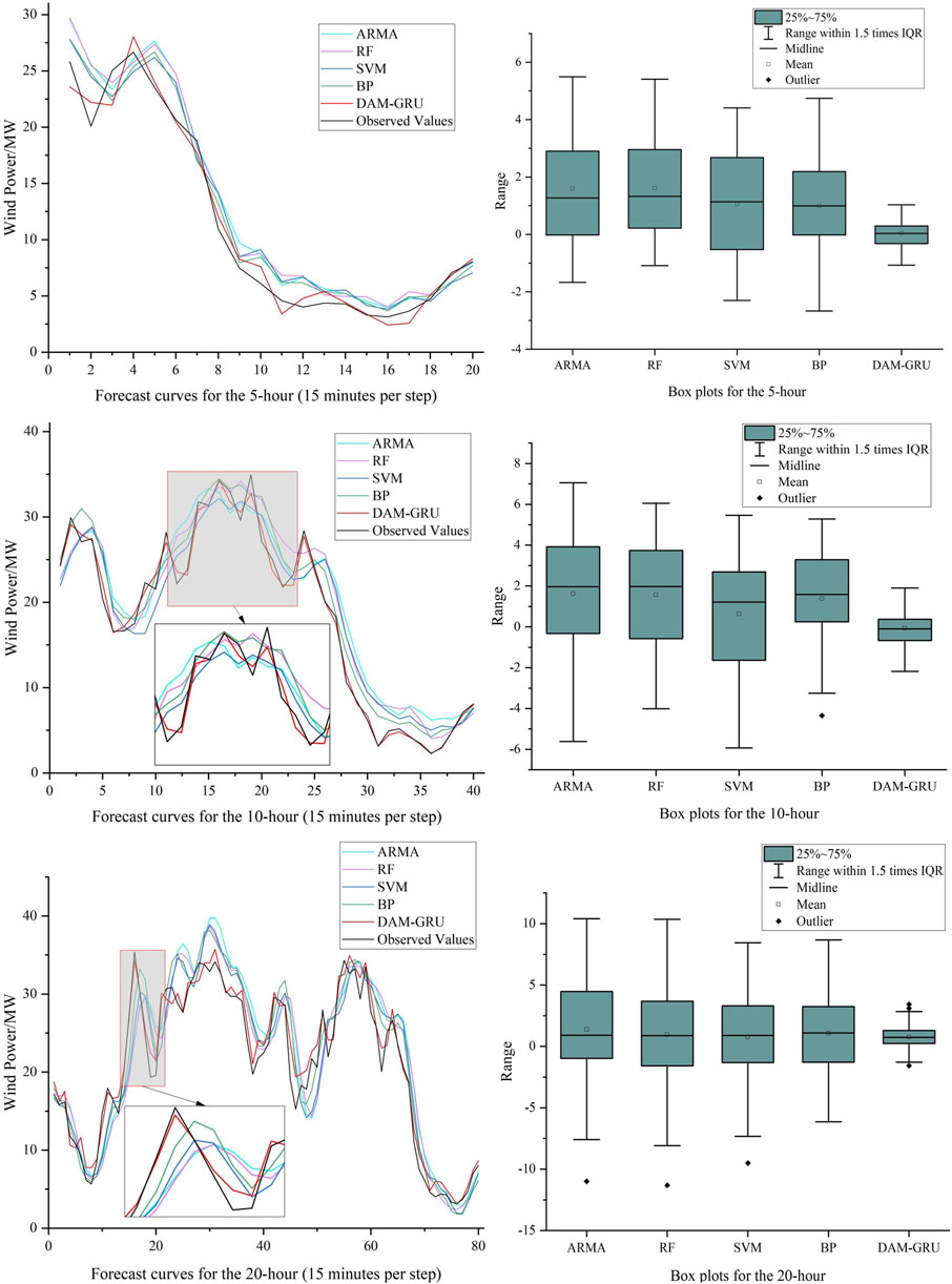
FIGURE 8. 5-h, 10-h and 20-h forecast curves and box plots for 5 models including ARMA, RF, SVM, BP, and DAM-GRU.

From Figure 8 it can be seen that the ARMA model is slightly stable at 5 h, but the error increases significantly as the prediction time increases, which may be less suitable for long-term forecasting. The three models, RF, SVM and BP, also show significant lags and do not fit the observed curves well at the peaks, where power changes more frequently. The DAM-GRU model proposed in this paper is able to accurately capture most of the large power variations and achieve accurate forecasts. This shows that the ideas and time-series feature processing methods specifically designed for wind power forecasting can make good use of historical data and capture the patterns embedded in longer time periods. Combining Tables 6, 7, it can be seen that although the proposed model has about twice the training and prediction time, its accuracy has improved significantly. As hardware performance improves, the training time for the model will be reduced even further in the future.

TABLE 6

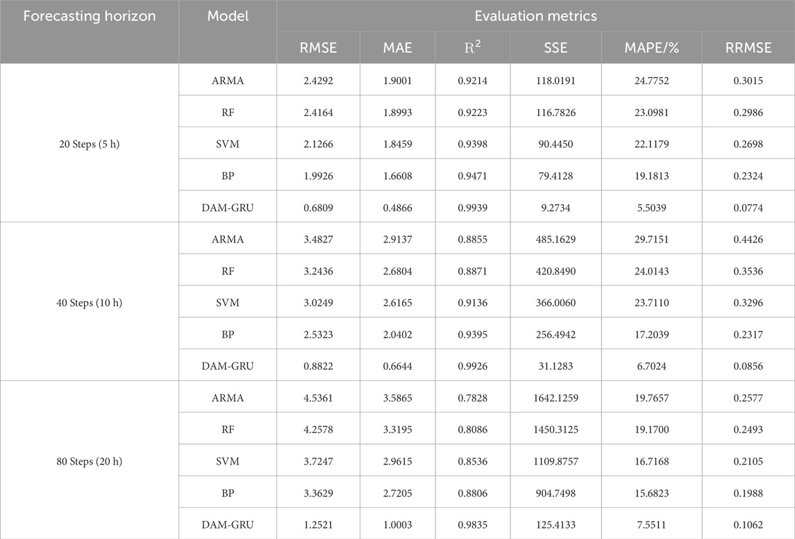
TABLE 6. Comparison of multi-stage forecasting errors with traditional models.

TABLE 7

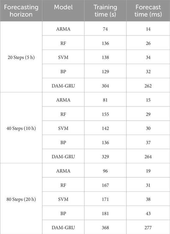
TABLE 7. Comparison of training time and forecasting time with traditional models.

5 Conclusion

Highly precise wind power forecasting is essential. Specifically, from the energy and environmental perspectives, it is conducive to the efficient utilization of wind power and the reduction of global carbon emissions; from the grid perspective, it is beneficial to the operator’s response to the fluctuation of wind power and the rational allocation of power. In order to achieve this goal through both real-time feature selection and time complexity reduction, we propose a DAM-GRU model and derive the following conclusions:

1. The results of the comparative experiments show that the introduction of the FAM in this study effectively extracts features contributing significantly to the point being forecast, thus enhancing short-term wind power forecasting accuracy.

2. One-dimensional convolutions with different kernel sizes provide filtering effects, reducing the complexity of the wind power sequences in individual channels and making forecasts less challenging for the model.

3. The temporal attention mechanism extracts crucial temporal features of preliminary forecasts at different time steps, while the addition of MHTAM helps the GRU network extract significant temporal features from multiple channels.

The proposed DAM-GRU algorithm is investigated with measured wind power data from a wind farm in Inner Mongolia, and better forecasting results are obtained, which will provide an effective basis for the construction of new wind farms in the neighbourhood. For example, accurate wind power forecasting will reduce the pressure on nearby peak frequency regulation power plants and increase the installed capacity of wind power generation, as well as facilitate the measurement of operating costs and the development of maintenance plans for the newly built wind power plants. However, this study also has the shortcoming that the setting of hyperparameters is based on the tuning experiment, which may cause the model to fall into local optimisation. In addition, the study is insufficient for the generalisation ability of the model. In the future, we will take the optimisation algorithm and the generalisation ability test as a breakthrough point to improve the model.

Data availability statement

The data analyzed in this study is subject to the following licenses/restrictions: The raw data supporting the conclusions of this article will be made available by the authors, without undue reservation. Requests to access these datasets should be directed to YL, 21214037870025@ymu.edu.cn.

Author contributions

WX: Funding acquisition, Software, Writing–review and editing. YL: Methodology, Writing–original draft. XF: Validation, Writing–review and editing. ZS: Writing–original draft. QW: Writing–review and editing.

Funding

The author(s) declare financial support was received for the research, authorship, and/or publication of this article. This work is supported by the National Natural Science Foundation of China (U1802271), and by the Ethnic and Religious Affairs Commission of Yunnan Province (2023YNMW010).

Conflict of interest

The authors declare that the research was conducted in the absence of any commercial or financial relationships that could be construed as a potential conflict of interest.

Publisher’s note

All claims expressed in this article are solely those of the authors and do not necessarily represent those of their affiliated organizations, or those of the publisher, the editors and the reviewers. Any product that may be evaluated in this article, or claim that may be made by its manufacturer, is not guaranteed or endorsed by the publisher.

References

Abdoos, A. A. (2016). A new intelligent method based on combination of vmd and elm for short term wind power forecasting. Neurocomputing 203, 111–120. doi:10.1016/j.neucom.2016.03.054

CrossRef Full Text | Google Scholar

Altan, A., Karasu, S., and Zio, E. (2021). A new hybrid model for wind speed forecasting combining long short-term memory neural network, decomposition methods and grey wolf optimizer. Appl. Soft Comput. 100, 106996. doi:10.1016/j.asoc.2020.106996

CrossRef Full Text | Google Scholar

Chi, D., and Yang, C. (2023). Wind power prediction based on wt-bigru-attention-tcn model. Front. Energy Res. 11, 1156007. doi:10.3389/fenrg.2023.1156007

CrossRef Full Text | Google Scholar

Couto, A., and Estanqueiro, A. (2022). Enhancing wind power forecast accuracy using the weather research and forecasting numerical model-based features and artificial neuronal networks. Renew. Energy 201, 1076–1085. doi:10.1016/j.renene.2022.11.022

CrossRef Full Text | Google Scholar

Duan, J., Wang, P., Ma, W., Tian, X., Fang, S., Cheng, Y., et al. (2021). Short-term wind power forecasting using the hybrid model of improved variational mode decomposition and correntropy long short-term memory neural network. Energy 214, 118980. doi:10.1016/j.energy.2020.118980

CrossRef Full Text | Google Scholar

Farah, S., David A, W., Humaira, N., Aneela, Z., Steffen, E., et al. (2022). Short-term multi-hour ahead country-wide wind power prediction for Germany using gated recurrent unit deep learning. Renew. Sustain. Energy Rev. 167, 112700. doi:10.1016/j.rser.2022.112700

CrossRef Full Text | Google Scholar

Gao, J., Ye, X., Lei, X., Huang, B., Wang, X., and Wang, L. (2023). A multichannel-based cnn and gru method for short-term wind power prediction. Electronics 12, 4479. doi:10.3390/electronics12214479

CrossRef Full Text | Google Scholar

Giebel, G., and Kariniotakis, G. (2017). Wind power forecasting—a review of the state of the art. Renew. energy Forecast., 59–109. doi:10.1016/b978-0-08-100504-0.00003-2

CrossRef Full Text | Google Scholar

He, Y., and Wang, Y. (2021). Short-term wind power prediction based on eemd–lasso–qrnn model. Appl. Soft Comput. 105, 107288. doi:10.1016/j.asoc.2021.107288

CrossRef Full Text | Google Scholar

Huang, B., Liang, Y., and Qiu, X. (2021). Wind power forecasting using attention-based recurrent neural networks: a comparative study. IEEE Access 9, 40432–40444. doi:10.1109/access.2021.3065502

CrossRef Full Text | Google Scholar

Huang, X., Zhang, Y., Liu, J., Zhang, X., and Liu, S. (2023). A short-term wind power forecasting model based on 3d convolutional neural network–gated recurrent unit. Sustainability 15, 14171. doi:10.3390/su151914171

CrossRef Full Text | Google Scholar

Lin, Y., Zhang, H., Liu, J., Ju, W., Wang, J., and Chen, X. (2021). “Research on short-term wind power prediction of gru based on similar days. J. Phys.: Conf. Ser. 2087, 012089. doi:10.1088/1742-6596/2087/1/012089

CrossRef Full Text | Google Scholar

Liu, J., Wang, X., and Lu, Y. (2017). A novel hybrid methodology for short-term wind power forecasting based on adaptive neuro-fuzzy inference system. Renew. energy 103, 620–629. doi:10.1016/j.renene.2016.10.074

CrossRef Full Text | Google Scholar

Liu, L., Liu, J., Ye, Y., Liu, H., Chen, K., Li, D., et al. (2023). Ultra-short-term wind power forecasting based on deep bayesian model with uncertainty. Renew. Energy 205, 598–607. doi:10.1016/j.renene.2023.01.038

CrossRef Full Text | Google Scholar

Liu, X., Yang, L., and Zhang, Z. (2021). Short-term multi-step ahead wind power predictions based on a novel deep convolutional recurrent network method. IEEE Trans. Sustain. Energy 12, 1820–1833. doi:10.1109/tste.2021.3067436

CrossRef Full Text | Google Scholar

Liu, X., Yang, L., and Zhang, Z. (2022). The attention-assisted ordinary differential equation networks for short-term probabilistic wind power predictions. Appl. Energy 324, 119794. doi:10.1016/j.apenergy.2022.119794

CrossRef Full Text | Google Scholar

Liu, X., and Zhou, J. (2024). Short-term wind power forecasting based on multivariate/multi-step lstm with temporal feature attention mechanism. Appl. Soft Comput. 150, 111050. doi:10.1016/j.asoc.2023.111050

CrossRef Full Text | Google Scholar

Meng, A., Chen, S., Ou, Z., Ding, W., Zhou, H., Fan, J., et al. (2022). A hybrid deep learning architecture for wind power prediction based on bi-attention mechanism and crisscross optimization. Energy 238, 121795. doi:10.1016/j.energy.2021.121795

CrossRef Full Text | Google Scholar

Saini, V. K., Bhardwaj, B., Gupta, V., Kumar, R., and Mathur, A. (2020). “Gated recurrent unit (gru) based short term forecasting for wind energy estimation,” in 2020 International Conference on Power, Energy, Control and Transmission Systems (ICPECTS) (IEEE), 1–6.

CrossRef Full Text | Google Scholar

Santhosh, M., Venkaiah, C., and Kumar, D. V. (2018). Ensemble empirical mode decomposition based adaptive wavelet neural network method for wind speed prediction. Energy Convers. Manag. 168, 482–493. doi:10.1016/j.enconman.2018.04.099

CrossRef Full Text | Google Scholar

Shih, S.-Y., Sun, F.-K., and Lee, H.-y. (2019). Temporal pattern attention for multivariate time series forecasting. Mach. Learn. 108, 1421–1441. doi:10.1007/s10994-019-05815-0

CrossRef Full Text | Google Scholar

Sun, Q., Duan, L., Liang, H., Zhao, C., and Lu, N. (2023). Design of a wind power forecasting system based on deep learning. J. Phys.: Conf. Ser. 2562, 012043. doi:10.1088/1742-6596/2562/1/012043

CrossRef Full Text | Google Scholar

Sun, Z., and Zhao, M. (2020). Short-term wind power forecasting based on vmd decomposition, convlstm networks and error analysis. IEEE Access 8, 134422–134434. doi:10.1109/access.2020.3011060

CrossRef Full Text | Google Scholar

Tian, Z. (2020). Backtracking search optimization algorithm-based least square support vector machine and its applications. Eng. Appl. Artif. Intell. 94, 103801. doi:10.1016/j.engappai.2020.103801

CrossRef Full Text | Google Scholar

Tian, Z. (2021). Modes decomposition forecasting approach for ultra-short-term wind speed. Appl. Soft Comput. 105, 107303. doi:10.1016/j.asoc.2021.107303

CrossRef Full Text | Google Scholar

Tian, Z., and Chen, H. (2021a). Multi-step short-term wind speed prediction based on integrated multi-model fusion. Appl. Energy 298, 117248. doi:10.1016/j.apenergy.2021.117248

CrossRef Full Text | Google Scholar

Tian, Z., and Chen, H. (2021b). A novel decomposition-ensemble prediction model for ultra-short-term wind speed. Energy Convers. Manag. 248, 114775. doi:10.1016/j.enconman.2021.114775

CrossRef Full Text | Google Scholar

Tian, Z., Li, H., and Li, F. (2021). A combination forecasting model of wind speed based on decomposition. Energy Rep. 7, 1217–1233. doi:10.1016/j.egyr.2021.02.002

CrossRef Full Text | Google Scholar

Tian, Z., Li, S., and Wang, Y. (2020). A prediction approach using ensemble empirical mode decomposition-permutation entropy and regularized extreme learning machine for short-term wind speed. Wind Energy 23, 177–206. doi:10.1002/we.2422

CrossRef Full Text | Google Scholar

van Heerden, L., Vermeulen, H., and van Staden, C. (2022). “Wind power forecasting using hybrid recurrent neural networks with empirical mode decomposition,” in 2022 IEEE International Conference on Environment and Electrical Engineering and 2022 IEEE Industrial and Commercial Power Systems Europe (EEEIC/I&CPS Europe) (IEEE), 1–6.

CrossRef Full Text | Google Scholar

Wang, Y., Xu, H., Zou, R., Zhang, L., and Zhang, F. (2022). A deep asymmetric laplace neural network for deterministic and probabilistic wind power forecasting. Renew. Energy 196, 497–517. doi:10.1016/j.renene.2022.07.009

CrossRef Full Text | Google Scholar

Wang, Y., Zou, R., Liu, F., Zhang, L., and Liu, Q. (2021). A review of wind speed and wind power forecasting with deep neural networks. Appl. Energy 304, 117766. doi:10.1016/j.apenergy.2021.117766

CrossRef Full Text | Google Scholar

Xiao, Y., Zou, C., Chi, H., and Fang, R. (2023). Boosted gru model for short-term forecasting of wind power with feature-weighted principal component analysis. Energy 267, 126503. doi:10.1016/j.energy.2022.126503

CrossRef Full Text | Google Scholar

Yang, B., Tu, Z., Wong, D. F., Meng, F., Chao, L. S., and Zhang, T. (2018). Modeling localness for self-attention networks. arXiv preprint arXiv:1810.10182.

Google Scholar

Yang, L., and Zhang, Z. (2021). A deep attention convolutional recurrent network assisted by k-shape clustering and enhanced memory for short term wind speed predictions. IEEE Trans. Sustain. Energy 13, 856–867. doi:10.1109/tste.2021.3135278

CrossRef Full Text | Google Scholar

Yang, L., Zheng, Z., and Zhang, Z. (2021). An improved mixture density network via wasserstein distance based adversarial learning for probabilistic wind speed predictions. IEEE Trans. Sustain. Energy 13, 755–766. doi:10.1109/tste.2021.3131522

CrossRef Full Text | Google Scholar

Zhang, H., Yan, J., Liu, Y., Gao, Y., Han, S., and Li, L. (2021). Multi-source and temporal attention network for probabilistic wind power prediction. IEEE Trans. Sustain. Energy 12, 2205–2218. doi:10.1109/tste.2021.3086851

CrossRef Full Text | Google Scholar

Zhang, Y., Pan, G., Chen, B., Han, J., Zhao, Y., and Zhang, C. (2020). Short-term wind speed prediction model based on ga-ann improved by vmd. Renew. Energy 156, 1373–1388. doi:10.1016/j.renene.2019.12.047

CrossRef Full Text | Google Scholar

Zhao, Z., Yun, S., Jia, L., Guo, J., Meng, Y., He, N., et al. (2023). Hybrid vmd-cnn-gru-based model for short-term forecasting of wind power considering spatio-temporal features. Eng. Appl. Artif. Intell. 121, 105982. doi:10.1016/j.engappai.2023.105982

CrossRef Full Text | Google Scholar