Stochastic optimal allocation for a battery energy storage system in high renewable-penetrated distribution networks

As the penetration of renewable distributed generation (RDG) continues to grow, the stochastic and intermittent nature of its output imposes significant challenges on distribution networks (DNs), such as source–load mismatch and voltage fluctuations, which seriously affects the safety and reliability of the system. Thus, this paper presents a stochastic optimal allocation method for a battery energy storage system (BESS) in the DN, with the consideration of annual load growth, BESS degradation, and DN operation, aiming to minimize the overall cost of DNs and harvest more renewable energy. Based on the rainflow-counting concept, BESS degradation is efficiently modeled and linearized to improve solvability. Additionally, to address the uncertainties of RDG outputs and loads, a stochastic optimization (SO) method is adopted. Furthermore, considering that a large number of integer variables of the BESS allocation model may cause a heavy computational burden, a feasibility pump-based solution algorithm is introduced to accelerate the solving speed. Finally, the effectiveness of the proposed BESS allocation method and the solution algorithm is verified on a 33-bus DN system through comparative analyses, showing high efficiency and performance.

1 Introduction

The integration of high penetration of renewable distributed generation (RDG) in a distributed network (DN) can bring technical challenges, particularly the voltage rise and line overload caused by the RDG power injection. These problems impose more stress on traditional regulation equipment in DN and affect the economy and stability of the distribution system.

Installing battery energy storage systems (BESSs) in DN is one of the promising solutions. BESS characterizes the features of high flexibility, rapid response, and less geographical restriction, which can effectively dampen the output fluctuation and intermittency of large-scale renewable energy (Hidalgo-León et al., 2017). However, the placement and sizing of BESS are two crucial factors that influence the performance of BESS application (Li et al., 2023; Yang et al., 2023). Given this, the optimal allocation of BESS in DN has received significant attention (Zhang and Wang, 2022).

In general, the existing literature on BESS allocation primarily focuses on the economic or security aspects of DN, with system operating constraints (Mohseni-Bonab et al., 2020; Zheng et al., 2020; Zhao et al., 2023). Meng et al. (2023) proposed a bi-level model for minimizing the total cost of DN based on the AC/DC hybrid DN topology, but it does not consider the placement optimization of BESS. Additionally, an optimal sizing and siting strategy of BESS in a high wind-penetrated power system has been suggested by Zhang et al. (2023a) to minimize the BESS investment cost. Taha et al. (2022) developed a multi-objective optimization planning model to minimize the average power loss and voltage fluctuation by optimizing the allocation of RDGs, BESS, and capacitor banks. Meanwhile, the three-phase power unbalance of DN is considered an objective for BESS allocation, and the future PV installation is treated as an uncertainty by Wang et al. (2021). However, these studies do not account for the impact of BESS degradation. In practice, unregulated charge or discharge behaviors can lead to battery lifespan deterioration, which can have adverse effects on the long-term reliable operation of BESS (Wang et al., 2020).

Currently, extensive research has been conducted on BESS degradation. Farzin et al. (2016) and Ju et al. (2018) investigated the lifespan degradation of BESS and found a direct correlation between the lifespan and depth of discharge (DOD). Mohsenian-Rad et al. (2016) restricted the number of cycles that a BESS can operate per day to ensure the battery lifespan, but it lessens the operational flexibility of BESS. Moreover, Zhang et al. (2021a) incorporated BESS degradation costs into a robust optimization (RO) model, and it assumes the uniform costs for each discharge cycle. In addition, the degradation cost caused by each discharge cycle is considered the function of DOD in Wang et al. (2020), enabling the calculation of the varying degradation costs of BESS. However, the aforementioned literature simplified the quantification of the number of BESS discharge cycles by equating it with the number of discharge, which may not accurately reflect the complete discharge cycle. In order to achieve the precise quantification of the total number of complete discharge cycles in BESS, the rainflow-counting method is commonly employed in practical engineering applications (Huang et al., 2021). This method emulates the flow of raindrops by analyzing the charge and discharge trajectory of BESS, thereby facilitating an accurate determination of the BESS cycle count (Xu et al., 2018a). However, it is important to note that the rainflow method lacks an analytical mathematical expression and cannot be directly integrated into the BESS allocation problem (Schneider et al., 2021). To address this limitation, the BESS degradation model has been decomposed in He et al. (2016) to iteratively optimize the BESS market quotation. However, this approach introduces numerous nonlinear terms, such as power functions and absolute value functions, which may lead to increased computational complexity. Additionally, Xu et al. (2018a) proposed a BESS operating model based on the rainflow method to optimize its charge and discharge for participation in the auxiliary frequency regulation market, but the newly introduced binary variables also add to the computational burden. Moreover, the deterioration of BESS capacity is also a notable consideration in the allocation problem of BESS (Ochoa-Barragán et al., 2023). However, there is a lack of inclusion of BESS capacity degradation in the operational models of the existing BESS allocation literature. Therefore, this study aimed to comprehensively account for the cost of BESS degradation based on the rainflow method in its allocation model. Additionally, the impact of capacity fade will be incorporated into the BESS operational model to reflect the practical situation for the BESS long-term operation.

Moreover, the uncertainties of RDG outputs and loads are also highly influencing the BESS planning stage. To address this issue, RO (Zhang et al., 2023b) and stochastic optimization (SO) (Hua et al., 2022) methods are often applied. RO constructs the uncertainty sets based on the upper and lower limits of uncertainty fluctuations and search for the worst case within the uncertainty sets to obtain an optimal solution under the worst case of uncertainty realization. Wang et al. (2021) proposed an RO allocation method for BESSs to improve the hosting capacity of the unbalanced three-phase DNs. However, the result obtained by the RO method could be conservative. On the other hand, Li and Grossmann (2021) and Pamshetti et al. (2022) introduced the SO method which produces numerous sampled scenarios to model the uncertainties based on their probability distribution and optimizes the decision variables with these sampled scenarios. In Li and Grossmann (2021), the SO method is compared with the RO method, and it concludes that SO is efficient when the goal is to optimize the expected outcome, and the problem can be modeled using probability distribution. Pamshetti et al. (2022) applied SO to solve the allocation problem of soft open point and BESS, considering the uncertainties of PV and load. The scenarios are produced using Monte Carlo simulation and employ the K-means clustering technique to determine the reduced scenarios with high quality and diversity. Considering that planning tends to find the optimal target expectation and the SO method is in line with this feature, so it is adopted in this paper.

Furthermore, the installation and operation of BESS, as well as the power flow model, typically involve a large number of integer variables and nonlinear terms (Cheng et al., 2023), which leads to a large computational burden and solving time. This will become serious with the application of SO, in which multiple scenarios are generated to represent the uncertainty realization. Therefore, it is necessary to explore an efficient solution algorithm. Some works adopt second-order cone relaxation and piecewise linearization methods to accelerate the computing speed (Shao et al., 2020; Mohamad et al., 2021; Wang et al., 2022), but they are still unable to efficiently address the issue caused by a large number of integer variables. Fischetti et al. (2005) proposed a feasible pump (FP) algorithm to deal with integer variables using a relax-and-rounding strategy. This strategy is also successfully utilized by Zhang et al. (2021b) to address the battery charge–discharge complementarity. Considering the advantage of the FP algorithm, it is therefore applied to address the integer variable problem in this paper.

Through the above literature review, it is found that the BESS degradation model in the allocation problem is not fully modeled, and the existing works do not comprehensively consider capacity fade, BESS degradation, annual growth, and uncertainty of DG and load in BESS allocation issues. Meanwhile, the integer problem in BESS allocation cannot be efficiently solved. Thus, this paper introduces a BESS allocation method in highly renewable-penetrated DNs, considering the factors mentioned above. The main contributions of this paper are summarized as follows:

(1) A stochastic optimal allocation approach of BESS in high renewable-penetrated DNs is proposed, aiming to minimize the overall cost and improve renewable power accommodation. The annual growth of RDG capacity and loads, as well as their uncertainties, is fully considered. Moreover, the battery degradation cost based on the rainflow-counting method and capacity fade is accurately modeled, and the nonlinear terms are efficiently linearized.

(2) To address the issue of slow solving speed due to numerous integer variables in the proposed BESS allocation model with SO, an FP-based algorithm is proposed. In this solution algorithm, the original stochastic BESS allocation problem is converted into a relaxed linear programming (LP) problem, which provides an initial solution. Then, the FP-rounding problem and integer flipping procedure are iteratively implemented until the feasible integer solution is obtained. The high efficiency of the proposed FP-based algorithm is demonstrated in this case study.

2 Mathematical formulation

This section introduces the proposed BESS allocation model. It not only determines the location and capacity of BESSs in DN but also simulates the operation of BESSs and DNs.

2.1 Objective function

The objective function (OF) of the proposed BESS allocation method is to minimize the total cost of DNs and harvest more renewable energy, which is expressed as follows:

$\min OF=\stackrel{A}{\overbrace{IC}}+\stackrel{B}{\overbrace{OC+DC+EPC}}+\stackrel{C}{\overbrace{EA}},(1)$

where Part A in Eq. 1 represents the investment cost (IC) of BESS; Part B stands for the total operating costs (e.g., operating cost, degradation cost of BESS, and energy trading cost); and Part C denotes the goal of renewable power accommodation.

First, the mathematical expression of IC is given as follows:

$\mathit{I}\mathit{C}={\mathit{E}\mathit{A}\mathit{C}}^{\mathit{b}\mathit{e}\mathit{s}\mathit{s}}\sum _{\mathit{i}\in {\mathrm{\Omega }}_{\mathit{b}\mathit{e}\mathit{s}\mathit{s}}}{\mathit{C}}_{\mathit{E},\mathit{b}\mathit{e}\mathit{s}\mathit{s}}^{\mathit{i}\mathit{n}\mathit{v}}{\mathit{E}}_{\mathit{i},\mathit{c}\mathit{a}\mathit{p},1}^{\mathit{b}\mathit{e}\mathit{s}\mathit{s}},(2)$

where ${\mathrm{\Omega }}_{bess}$ represents the set of nodes for BESS installation; ${EAC}^{bess}$ represents the equivalent annual investment cost of BESS, which can be defined in Eq. 3, where $r$ represents the discount rate and $y$ is the BESS economic life. $C_{E,bess}^{inv}$ denotes the unit capacity cost of BESS, and $E_{i,cap,1}^{bess}$ indicates the installed capacity of BESS.

${EAC}^{bess}=\frac{r{\left(1+r\right)}^y}{{\left(1+r\right)}^y-1}.(3)$

Meanwhile, Part B in Eq. 1 denotes the total operating cost of DN, whose mathematical expression is determined as follows:

$OC=\sum _{y=1}^Y\sum _{t=1}^{T}365\left(C_{bess}^{OM}\sum _{i\in {\mathrm{\Omega }}_{bess}}\left(P_{i,y,t}^{ch}{\eta }_{bess}^{ch}+P_{i,y,t}^{dis}{/\eta }_{bess}^{dis}\right)\right),(4)$

$EPC=\sum _{y=1}^Y\sum _{t=1}^{T}365\left(P_{t,y}^{buy}{P}_{t,y}^{\mathit{def}}-P_{t,y}^{sell}{P}_{t,y}^{suf}\right),(5)$

$DC=\sum _{i{\in \mathrm{\Omega }}_{bess}}\sum _{y=1}^Y\sum _{t=1}^T\sum _{j=1}^J{c}_j{P}_{i,y,t,j}^{dis}.(6)$

Equation 4 represents the operation cost of BESS, $Y$ is the planning year, and $T$ is the duration of a day in the planning scenario. $P_{i,t,y}^{ch/dis}$ represents the charge/discharge power of BESS, and ${\eta }_{bess}^{ch/dis}$ represents the charge/discharge efficiency. $C_{bess}^{OM}$ represents the operating cost per unit power of BESS. Equation 5 represents the energy trading cost, ${\mathit{Pr}}_{t,y}^{buy/sell}$ represents the buying/selling price, and $P_{t,y}^{\mathit{def}/suf}$ represents the energy trading power of DN.

Equation 6 represents the degradation cost of BESS. In this paper, considering that the amounts of energy charged and discharged from a BESS are almost the same per day (Chen, 2023), for simplicity, we assume that full-cycle aging degradation only occurs during the BESS discharge stage of a cycle. As a result, the degradation cost of BESS can be defined as the product of the discharge power $P_{i,y,t.j}^{dis}$ and marginal degradation cost $c_j$ of BESS. It is noted that, in order to mitigate the impact of the nonlinear components of the BESS degradation model, this study has utilized the piecewise linearization method to divide $P_{i,y,t}^{dis}$ into five segments ($P_{i,y,t,j}^{dis}$, j = 1,2,3 … 5), thereby approximating the model. A detail explanation of $DC$ can be found in Section 2.3.

In order to harvest more renewable energy in DN, penalty cost coefficients $C_{RDG}$ are introduced to minimize the curtailment of RDGs. Thus, the expression of the C component in Eq. 1 is shown as follows:

$EA=365\sum _{y=1}^Y\sum _{t=1}^T\left(\left(\sum _{i\in {\mathrm{\Omega }}_{RDG}}{C}_{RDG}{P}_{ab,i,y,t}^{RDG}\right)\right),(7)$

where ${\mathrm{\Omega }}_{RDG}$ represents the set of nodes for RDGs and $P_{ab,i,y,t}^{RDG}$ represents the curtailment power of RDGs.

2.2 Allocation model of BESS

The general BESS allocation constraints are modeled as follows:

${\alpha }_i{E}_{cap,\mathit{min}}^{bess}\le E_{i,cap,y}^{bess}\le {\alpha }_i{E}_{cap,\mathit{max}}^{bess},(8)$

$\sum _{i\in {\mathrm{\Omega }}_{bus}}{\alpha }_i\le N_{BSL},(9)$

$0\le P_{i,y,t}^{ch}\le \left(1-{\beta }_i\right)P_{\mathit{max}}^{bess},(10)$

$0\le P_{i,y,t}^{dis}\le {\beta }_i{P}_{\mathit{max}}^{bess},(11)$

$0\le P_{i,y,t}^{\frac{ch}{dis}}\mathrm{\tau }\le E_{cap,\mathit{max}}^{bess},(12)$

$E_{i,y,t}^{bess}=E_{i,y,t-1}^{bess}+P_{i,y,t}^{ch}{\eta }_{bess}^{ch}\mathrm{\tau }-P_{i,y,t}^{dis}\mathrm{\tau }/{\eta }_{bess}^{dis},(13)$

$E_{i,y,0}^{bess}=E_{i,y,24}^{bess},(14)$

$E_{i,cap,y}^{bess}{SOC}_{\mathit{min}}{\le E}_{i,y,t}^{bess}\le E_{i,cap,y}^{bess}{SOC}_{\mathit{max}},(15)$

where $\mathrm{\tau }$ represents the time period; ${\alpha }_i$ represents the binary decision variable for BESS installation; $N_{BSL}$ represents the maximum number for installation in DN; $P_{\mathit{max}}^{bess}$ represents the maximum charge/discharge power of BESS; $E_{i,cap,y}^{bess}$ represents the installed capacity; and ${SOC}_{\mathit{max}/\mathit{min}}$ represents the maximum/minimum SOC. ${\beta }_i$ represents a binary variable that indicates the mode of charge or discharge. If BESS is in the charge mode, ${\beta }_i$ will be 0, and if BESS is in the discharge mode, it will be one.

Constraints (8) and (9) limit the maximum BESS allocation power and the number of BESS installing positions. Constraints (10)–(12) limit the BESS charge/discharge power and ensure that at most one charge/discharge state can be active at each time interval. Equation 13 denotes the remaining energy of BESS after charge/discharge at each time interval. Equation 14 ensures that the energy in BESS at the last time of a day is equal to the initial energy, and constraint (15) limits the BESS state of charge (SOC) within the optimized upper and lower SOC limits.

2.3 Degradation model of BESS

2.3.1 Introduction of the rainflow-counting method

Considering that BESS degradation is highly related to the number of discharge cycles throughout its entire life cycle (Gräf et al., 2022). In order to obtain the discharge cycle set $M$ during BESS operation, the rainflow-counting method is applied in practice (Valentin et al., 2015). Figure 1 describes the process of cycle depth obtained using the rainflow method. As an example, the BESS SOC during the operation is shown in Figure 1A, and the result of a cycle depth of BESS is shown in Figure 1B, which can be obtained by the following sequence:

(1) Taking the first four points, namely, A, B, C, and D, their distance is calculated: $\Delta {\mathrm{S}}_{AB}=\left|A-B\right|$, $\Delta {\mathrm{S}}_{BC}=\left|B-C\right|$, and $\Delta {\mathrm{S}}_{CD}=\left|C-D\right|$.

(2) If $\Delta {\mathrm{S}}_{BC}\le \Delta {\mathrm{S}}_{AB}$ and $\Delta {\mathrm{S}}_{BC}\le \Delta {\mathrm{S}}_{CD}$, a full cycle of DOD $\Delta {\mathrm{S}}_{BC}$ (B–C–B′) will be obtained. Therefore, B and C will be removed and the calculation will be repeated with the points of A, D, E, and F.

(3) If the cycle is not obtained, the calculation is shifted forward and the calculation is repeated with points B, C, D, and E.

(4) The calculation will be repeated until no more cycles can be found throughout the remaining profile.

FIGURE 1

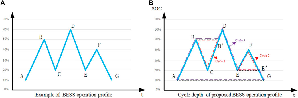
FIGURE 1. Illustration of BESS cycle depth by rainflow algorithm. (A) Example of BESS operation profile. (B) Cycle depth of proposed BESS operation profile.

According to the steps above, the three full cycles of depth 30% (B–C–B′), 20% (E–F–E′), and 50% (A–B–B′–D–E–E′–G) are obtained, as shown in Figure 1B. Thus, the cycle set $M$ will contain three discharge cycles: a 30% depth cycle of B–C, a 20% depth cycle of F–E′, and a 50% depth cycle of D–E–E′–G.

Then, the overall degradation expense of BESS can be considered the sum of the degradation costs incurred from each identified cycle determined using the rainflow-counting method. This is articulated as follows:

$\mathit{D}\mathit{C}=\sum _{\mathit{m}\in \mathit{M}}{\mathit{L}}_{\mathit{m}},(16)$

where $M$ represents the set of discharge cycles during BESS operation and $L_m$ represents the degradation cost in the $mth$ cycle.

2.3.2 Marginal degradation cost of BESS

The degradation of BESS during each discharge cycle is associated with its DOD (Ju et al., 2018). To describe the incremental degradation caused by different DODs, a cycle depth aging stress function $\mathrm{\Phi }\left({\delta }_{i,t}\right)$ has been defined (Xu et al., 2017), where a typical curve is shown in Figure 2. In addition, for the BESS allocation problem, in order to avoid nonlinear constraints, tracking the BESS discharge power is easier than DOD, so it is necessary to further explore the relationship between incremental degradation and discharge power in each cycle (Xu et al., 2018b).

FIGURE 2

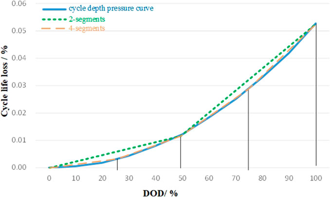
FIGURE 2. Typical cycle depth pressure curve.

In practical operation, if BESS is discharged from ${SOC}^{up}$ to ${SOC}^{end}$ and later charged back to ${SOC}^{up}$ (or vice versa), this process will be considered a discharge cycle, and the DOD ${\delta }_{i,t}$ and the discharge power $P_i^{dis}$ of this cycle can be expressed as $\left|{SOC}^{up}-{SOC}^{end}\right|$ and $\left|{SOC}^{up}-{SOC}^{end}\right|E_{i,cap}^{bess}$/$\mathrm{\tau }$, respectively, where $E_{i,cap}^{bess}$ represents the capacity of BESS. Then, during a cycle, assuming that the BESS will discharge $P_{i,t}^{dis}$ power from DOD ${\delta }_{i,t-1}$ at time $t$. The cycle depth of BESS at time t can be expressed in Eq. 17, and the incremental degradation in this cycle is $\mathrm{\Phi }\left({\delta }_{i,t}\right)$.

${\delta }_{i,t}=\frac{1}{{\eta }_{bess}^{dis}{E}_{i,cap}^{bess}}{P}_{i,t}^{dis}\mathrm{\tau }+{\delta }_{i,t-1}.(17)$

Then, to calculate the incremental degradation caused by discharging power, we can consider the derivative of $\mathrm{\Phi }\left({\delta }_{i,t}\right)$ with respect to $P_{i,t}^{dis}$, substituting from Eq. 17 as follows:

$\frac{\partial \mathrm{\Phi }\left({\delta }_{i,t}\right)}{\partial P_{i,t}^{dis}}=\frac{d\mathrm{\Phi }\left({\delta }_{i,t}\right)}{{d\delta }_{i,t}}\frac{{d\delta }_{i,t}}{d{P}_{i,t}^{dis}}=\frac{\mathrm{\tau }}{{\eta }_{bess}^{dis}{E}_{i,cap}^{bess}}\frac{d\mathrm{\Phi }\left({\delta }_{i,t}\right)}{{d\delta }_{i,t}}.(18)$

Through Eq. 18, the incremental degradation brought by unit discharge power is obtained. Additionally, considering that $\mathrm{\Phi }\left({\delta }_{i,t}\right)$ is a nonlinear function, for the sake of simplicity, this paper uses a piecewise linearization method to construct an approximation function $Cp\left({\delta }_{i,t}\right)$. This function evenly divides the cycle depth range (from 0% to 100%) into $J$ linear segments to achieve an approximation.

Then, $\frac{d\mathrm{\Phi }\left({\delta }_{i,t}\right)}{{d\delta }_{i,t}}$ in Eq. 18 is expressed as follows:

$\frac{d\mathrm{\Phi }\left({\delta }_{i,t}\right)}{{d\delta }_{i,t}}=\frac{dCp\left({\delta }_{i,t}\right)}{{d\delta }_{i,t}}=\left\{\begin{array}{cc}{k}_1& if{\delta }_{i,t}\in \left[0,\frac{1}{J}\right),\\ & ⋮\\ k_j& if{\delta }_{i,t}\in \left[\frac{j-1}{J}\right.,\frac{j}{J})\\ & ⋮\\ k_J& if{\delta }_{i,t}\in \left[\frac{j-1}{J},1\right],\end{array}\right.,(19)$

where $k_j$ is the slope of the linearized function of the $jth$ segment.

Finally, by converting the replacement cost $R=r{E}_{i,cap}^{bess}$ of BESS into the marginal degradation cost, the finally cycle degradation cost of BESS is expressed as follows:

$c_j=\frac{R\mathrm{\tau }}{{\eta }_{bess}^{dis}{E}_{i,cap}^{bess}}{k}_j=\frac{r\mathrm{\tau }}{{\eta }_{bess}^{dis}}{k}_j,(20)$

where $r$ represents the unit replacement cost of BESS. Based on the cycle degradation cost, the total degradation in the $mth$ cycle is expressed as follows:

${\mathit{L}}_{\mathit{m}}=\mathit{c}{\mathit{P}}_{\mathit{i},\mathit{t},\mathit{m}}^{\mathit{d}\mathit{i}\mathit{s}},(21)$

where $P_{i,t,m}^{dis}$ represents the discharge power in the $mth$ cycle and $c$ represents the set of the final cycle degradation cost $c_j\left(j=1,2,3\dots J\right)$.

2.3.3 BESS degradation model

It is worth noting that the cycle set $M$ obtained based on the rainflow method in Section 2.3.1 is derived from known trajectories and does not have an analytical mathematical expression, which presents challenges for its direct application within the allocation model. To accurately calculate the degradation cost caused by multiple discharge cycles during BESS operation, a BESS degradation model is constructed, aiming to achieve the approximation of the rainflow method (Xu et al., 2018a), whose expression is shown as follows:

$P_{i,y,t}^{dis}=\sum _{j=1}^J{P}_{i,y,t,j}^{dis},(22)$

$P_{i,y,t}^{ch}=\sum _{j=1}^J{P}_{i,y,t,j}^{ch},(23)$

${0\le P}_{i,y,t,j}^{ch}\le P_{\mathit{max}}^{bess},(24)$

${0\le P}_{i,y,t,j}^{dis}\le P_{\mathit{max}}^{bess},(25)$

$e_{i,y,t,j}^{bess}-e_{i,y,t-1,j}^{bess}=P_{i,y,t,j}^{ch}{\eta }_{bess}^{ch}\mathrm{\tau }-P_{i,y,t,j}^{dis}\mathrm{\tau }{\frac{}{\eta }}_{bess}^{dis},(26)$

$0\le e_{i,y,t,j}^{bess}\le {\stackrel{\sim }{e}}_{i,j},(27)$

${\stackrel{\sim }{e}}_{i,j}=\frac{1}{J}{E}_{i,cap,1}^{bess},(28)$

$E_{i,y,t}^{bess}=\sum _{j=1}^J{e}_{i,y,t,j}^{bess},(29)$

where $j$ represents the segment interval divided by the piecewise linearization method, as shown in Section 2.3.2. $P_{i,y,t,j}^{ch/dis}$ denotes the charge/discharge power; $e_{i,y,t,j}^{bess}$ represents the energy stored at time t, and ${\stackrel{\sim }{e}}_{i,j}$ represents the upper limit of the energy stored in the $jth$ segment.

Equations 22 and 23 denote the equivalent charge and discharge power, respectively. Constraints (24) and (25) limit the charge and discharge power for each segment, respectively. Equation 26 represents the amount of energy stored in the $jth$ segment. Constraints (27) and (28) set the upper and lower limits in the $jth$ segment, respectively, and the storage level of BESS is described in Eq. 29.

Considering that $\mathrm{\Phi }\left({\delta }_{i,t}\right)$ is convex, BESS will generally be charged or discharged from the shallowest segment to the deeper segment. Thus, constraints 22–29 can achieve a close approximation with the rainflow method, and the total degradation cost during BESS operating time is calculated in Eq. 6.

An example is shown to illustrate how the proposed BESS degradation model can make a close approximation of the rainflow method using the operation trajectory, as shown in Figure 1. In this example, we assume the detail function of $\mathrm{\Phi }\left(\delta \right)$ = $100{\delta }^2$, and the number of segments $J$ divided through piecewise linear approximation function is 10. For illustration and simplicity, the cost coefficient $\frac{r\mathrm{\tau }}{{\eta }_{bess}^{dis}}$ is also assumed as 1$/kW. Consequently, the cycle degradation cost of BESS is expressed as follows:

$c=\left[1,3,5,7,9,11,13,15,17,19\right].$

According to the rainflow method in Section 2.3.2, we observe that the trajectory shown in Figure 1B has three discharging cycles of 30%, 20%, and 50% depth, and the total degradation cost is 38 $. Then, we implement the operation profile based on the proposed method and record the degradation cost during each time interval through Eq. 6. The results are shown in Table 1.

TABLE 1

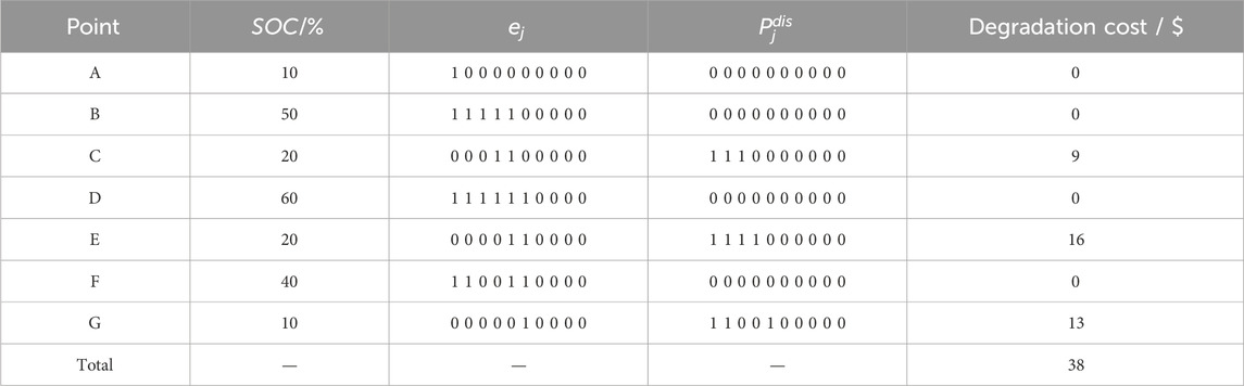
TABLE 1. Example of the proposed BESS degradation counting model.

In Table 1, the energy level of BESS is shown as a vector $e_j$ in the third column, which is a 10 × 1 vector, and its energy level is sorted from a shallower to deeper depth. Moreover, each segment is normalized; if the segment is full, it will be one, and if the segment is empty, it will be 0. Similarly, the discharge power of each segment is also shown as a 10 × 1 vector in the fourth column, and if the segment discharges 10% $E_{i,cap}^{bess}$ power, it will be one.

Through Table 1, we can find that, in the counting process of a discharge cycle (such as D–E–F–G), if a charge behavior occurs (E–F), the proposed model will restart discharge from the shallowest segment in the next discharge behavior and recounting the DOD of this new cycle until charge power is full released (F–E′). Then, the model will continue to calculate the DOD of the original cycle based on the previous discharge depth (E’) until the next charge behavior that occurs beyond the current DOD. This process is similar to the rainflow method, and the example results in the total degradation cost of 38 $ in both the proposed model and rainflow method.

2.4 Deterministic optimal allocation model for BESS

By combining the above BESS model and objective function, the optimal allocation model of BESS is obtained as follows:

$\min OF=IC+OC+DC+EPC+EA.(30)$

subject to (8)–(15) and (22)–(29)

$P_{i,y,t}=P_{i,y,t}^{LD}-P_{i,y,t}^{RDG}-P_{i,y,t}^{dis}+P_{i,y,t}^{ch},(31)$

$Q_{i,y,t}=Q_{i,y,t}^{LD},(32)$

$0\le P_{i,y,t}^{RDG}\le P_{i,y,t}^{RDG,pre},(33)$

$P_{ab,i,y,t}^{RDG}=P_{i,y,t}^{RDG,pre}-P_{i,y,t}^{RDG},(34)$

$\sum _{i\in u\left(j\right)}{P}_{ij,t}=\sum _{i\in v\left(j\right)}{P}_{ik,t}-P_{j,t},(35)$

$\sum _{i\in u\left(j\right)}{Q}_{ij,t}=\sum _{i\in v\left(j\right)}{Q}_{ik,t}-Q_{j,t},(36)$

$V_{j,t}=V_{i,t}-\frac{r_{ij}{P}_{ij,t}+x_{ij}{Q}_{ij,t}}{V_0},(37)$

$U_{\mathit{min}}\le U_{i.t}\le U_{\mathit{max}},(38)$

$P_{i,y,n}^{RDG}={\epsilon }_y^{RDG}{P}_{i,y-1,n}^{RDG},(39)$

$P_{i,y,n}^{LD}={\epsilon }_y^{LDP}{P}_{i,y-1,n}^{LD},(40)$

$Q_{i,y,n}^{LD}={\epsilon }_y^{LDQ}{Q}_{i,y-1,n}^{LD},(41)$

$E_{i,cap,y}^{bess}={\epsilon }_y^{bess}{E}_{i,cap,y-1}^{bess},(42)$

where Eqs 31 and 32 represent the injected power at node $i$, and $P_{i,y,t}^{LD}$, $Q_{i,y,t}^{LD}$, and $P_{i,y,t}^{RDG}$ represent the output power of the load and RDGs. Constraints (33) and (34) denote the curtailment constraints of RDGs, and $P_{i,y,t}^{RDG,pre}$ represents the predicted power. Equations 35–37 represent the power flow model of the system, and Eq. 38 limits the voltage value of bus nodes. Equations 39–41 propose the annual growth model for loads and RDGs in the system, where ${\epsilon }_y^{RDG}$, ${\epsilon }_y^{LDP}$, and ${\epsilon }_y^{LDQ}$ represent the annual growth rates for RDGs and loads. Equation 42 represents the degradation of BESS capacity, and ${\epsilon }_y^{bess}$ represents the annual capacity decay rate.

2.5 Stochastic optimization for the BESS allocation model

To address the uncertainties of RDGs and loads, a scenario-based two-stage SO method is applied. Considering that the probability distribution could be unknown or inaccurate, a sample average approximation method (Li et al., 2017) is used in this paper. Thus, the proposed model is expressed as follows:

$\min IC+\min \frac{1}{N_s}\sum _{u_s\in U}OC+DC+EPC+EA.(43)$

subject to (8)–(15), (22)–(29), and (31)–(42),

where $U$ represents the set of scenarios and $u_s$ represents the uncertain output of RDG and load under scenario $s$. $N_s$ represents the total number of scenarios in the set $U$.

Model (43) can be regarded as a two-stage optimization. The first stage is the minimization of the BESS allocation cost by optimizing BESS location and sizing in the DN, i.e., $\min IC$. The second stage represents the minimization of DN operation with the first-stage BESS allocation decisions, i.e., $\min \frac{1}{N_s}{\displaystyle \sum _{u_s\in U}}OC+DC+EPC+EA$. By combining these two stages together, Model (43) forms a two-stage optimization problem, indicating that BESS allocation is optimized with the consideration of a DN operation.

3 Solution algorithm

The BESS SO allocation model with integer variables proposed in Section 2.5 is expressed in the following compact form:

$\underset{x,z_1}{\min }{C}_1^{T}x+\frac{1}{N_s}\underset{u_s\in U,y_s{,z}_{2,s}}{\min }{C}_2^T{y}_s,(44)$

$\text{subject}\hspace{0.17em}\text{to}A\left[x;z_1\right]\ge b,(45)$

$D\left[x;z_1\right]+E\left[y_s;z_{2,s}\right]+Fu\ge v,(46)$

$G\left[x;z_1\right]+H\left[y_s;z_{2,s}\right]+Iu=\omega .(47)$

In Model (44), $x$ denotes the continuous decision variables $E_{i,cap,y}^{bess}$, while $z_1$ represents the integer decision variables ${\alpha }_i$ in the first stage. Then, $y_s$ signifies the continuous variables, including $P_{i,y,t,j}^{ch/dis}$, $P_{t,y}^{\mathit{def}}$, and $P_{t,y}^{sub}$, and other dependent variables. $z_{2,s}$ denotes the integer variable ${\beta }_i$ in the second stage. In addition, the first-stage inequality constraint (45) includes (8) and (9). Constraint (46) represents the inequality constraints in the second stage, including constraints (10)–(12), (15), (24), (25), (27), (33), and (38). Constraint (47) represents the other equality constraints in Model (43).

Model (44) is a typical MILP problem, which is often solved by commercial solvers, such as Gurobi and CPLEX. However, solving MILP problems with a large number of integer variables generally takes a long time. Therefore, it is crucial to balance between the solution optimal and solving time. This study is based on the FP algorithm to improve the solving efficiency of the MILP problem. The algorithm mainly comprises two parts: relaxed LP problem and FP-rounding problem. The specific handling methods are as follows.

First, let $z$ be the set of integer variables in the problem, which means $z=\left\{z_1;z_{2,s}\right\}$; then, by relaxing all integer variables into continuous variables $\stackrel{\sim }{z}$ and adding the following constraints, we obtain

$0\le {\stackrel{\sim }{z}}_j\le 1.(48)$

As a result, the relaxed LP problem can be formulated in the following manner:

$\underset{x,{\stackrel{\sim }{z}}_1}{\min }{C}_1^{T}x+\frac{1}{N_s}\underset{u\in U,y_s{,\stackrel{\sim }{z}}_{2,s}}{\min }{C}_2^T{y}_s.(49)$

subject to (48)

$A\left[x;{\stackrel{\sim }{z}}_1\right]\ge b,(50)$

$D\left[x;{\stackrel{\sim }{z}}_1\right]+E\left[y_s;{\stackrel{\sim }{z}}_{2,s}\right]+Fu\ge v,(51)$

$G\left[x;{\stackrel{\sim }{z}}_1\right]+H\left[y_s;{\stackrel{\sim }{z}}_{2,s}\right]+Iu=\omega .(52)$

Then, ${\stackrel{⃡}{z}}^{*}=\left[{\stackrel{\sim }{z}}^{*}\right]$ is used to round each integer variable in ${\stackrel{\sim }{z}}^{*}$ obtained from the relaxed LP problem, and the distance function between the continuous variables $\stackrel{\sim }{z}$ and the currently obtained integer variables is calculated ${\stackrel{⃡}{z}}^{*}$ as follows:

$\Delta \left(\stackrel{\sim }{z}\right)=\sum _{{\stackrel{⃡}{z}}_j^{*}=0}{\stackrel{\sim }{z}}_j+\sum _{{\stackrel{⃡}{z}}_j^{*}=1}\left(1-{\stackrel{\sim }{z}}_j\right).(53)$

Moreover, in order to obtain results by the FP algorithm close to the optimal solution, (44) and (53) are added as the objective function to form the FP-rounding problem as follows:

$\left\{\begin{array}{c}\underset{\stackrel{\sim }{z}}{\min }{\omega }_1\frac{\Delta \left(\stackrel{\sim }{z}\right)}{{\Delta \left(\stackrel{\sim }{z}\right)}_{\mathit{max}}}+\frac{{\omega }_2}{n_{iter}}\frac{F}{F_{\mathit{max}}}\\ F=\underset{x,{\stackrel{\sim }{z}}_1}{\min }{C}_1^{T}x+\frac{1}{N_s}\underset{u\in U,y_s{,\stackrel{\sim }{z}}_{2,s}}{\min }{C}_2^T{y}_s\\ \text{subject}\text{to}\left(48\right),\left(50\right)-\left(52\right),\end{array}\right.(54)$

where ${\omega }_1$ and ${\omega }_2$ represent weighting coefficients for each objective. $F$ represents the objective function of the original problem, and $n_{iter}$ represents the number of iterations of the proposed FP-based algorithm. By incorporating the $\frac{{\omega }_2}{n_{iter}}\frac{F}{F_{\mathit{max}}}$ component into the objective function, the results derived from the FP-rounding problem will be close to the optimal solution of the original problem. Additionally, as the number of iterations increases, the impact of F will diminish, thereby mitigating its influence on feasibility. Moreover, when $\frac{\Delta \left(\stackrel{\sim }{z}\right)}{{\Delta \left(\stackrel{\sim }{z}\right)}_{\mathit{max}}}$ reaches the minimum value 0, $F$ will also obtain the relatively minimal values, which can be considered an acceptable optimal result for the original MILP problem.

Then, the new solution ${\stackrel{\sim }{z}}^{*}$ obtained from the FP-rounding problem is rounded to obtain a rounded integer solution ${\stackrel{⃡}{z}}^{*}$, and the distance function $s={\displaystyle \sum _{i=1}^I}\left|{\stackrel{⃡}{z}}^{*}-{\stackrel{\sim }{z}}^{*}\right|$ is calculated. The role of $s$ is to determine the distance between ${\stackrel{\sim }{z}}^{*}$ and ${\stackrel{⃡}{z}}^{*}$; the smaller $s$ is, the closer ${\stackrel{\sim }{z}}^{*}$ is to the integer solution; and when $s=0$, ${\stackrel{\sim }{z}}^{*}$ will be the final feasibility solution. Moreover, if $s>0$, the rounded integer solution ${\stackrel{⃡}{z}}^{*}$ will be used for the next FP-rounding problem.

Furthermore, to avoid stalling issues, it is necessary to flip a random set of $RN\left(RN\in \left[\overline{RN},\underset{\_}{RN}\right]\right)$ variables in the integer flipping procedure. It is worth noting that the lower and upper bounds of the random number are expected to be set with the consideration of the optimization problem size. The larger the problem is, the larger the range should be. The detail instruction of the bound setting can be found in Fischetti et al. (2005).

The iteration continues to solve the FP-rounding problem and integer flipping procedure until an integer solution is obtained. During the solving process, the algorithm either returns an infeasible result or the optimal integer solution for the original MILP problem. The solving process for the stochastic BESS allocation model based on the FP algorithm is shown in Figure 3.

FIGURE 3

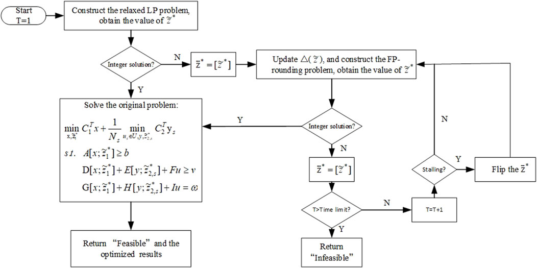
FIGURE 3. Solving process.

4 Case study

4.1 System setting

To verify the effectiveness of the proposed BESS SO allocation approach, a 33-bus system is applied, and its topology is shown in Figure 4. The typical RDGs and load output for the four seasons are shown in Figure 5, which are regarded as the expected condition. The prediction bounds are set as ± 20% of the RDG output and ± 10% of load output. Then, 100 scenarios are obtained through Monte Carlo random sampling in these bounds for SO application. In addition, the rated power and location of each RDGs are shown in Table 2.

FIGURE 4

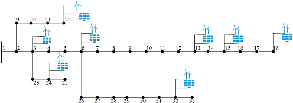
FIGURE 4. Topology of a 33-bus DN system.

FIGURE 5

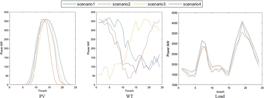
FIGURE 5. Typical RDGs and load output for the four seasons.

TABLE 2

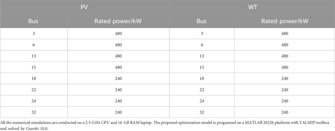
TABLE 2. Bus location and rated power of RDGs.

The specific calculation conditions are described as follows:

(1) The penalty cost of curtailment RDGs is 0.83 $/kW (Yan et al., 2022).

(2) The unit capacity cost of energy storage is 2,000 $/kW h (Yan et al., 2022).

(3) The planning cycle is 10 years, and the annual capacity decay rate is set as 2%.

(4) The alternative points for BESS are nodes 3, 6, 13, 15, 18, 22, 24, and 32, and the maximum number of installation nodes for BESS is 4.

(5) The maximum installation capacity of BESS is 2 MW h, and the minimum is 200 kW h.

(6) The setting categories of time-of-use electricity prices are as follows: the peak hour electricity price is 0.93 $/kW between 9:00 and 13:00 and 18:00 and 21:00. The valley hour electricity price is 0.31 $/kW between 22:00 and 5:00, and the normal electricity price is 0.62 $/kW between 6:00 and 8:00 and 14:00 and 17:00.

(7) The setting categories of electricity sales price are 0.3 times the time-of-use electricity prices.

(8) The voltage range is set as 0.95–1.05 p.u.

4.2 Results and performance comparison

4.2.1 BESS allocation in DN

Without considering the BESS allocation, the penalty cost for RDG curtailment in the DN is shown in Table 3. Moreover, the BESS allocation results obtained by the proposed model are shown in Figure 6. By installing BESS at buses 13, 15, 18, and 32, we can achieve the total cost at 25.66 $ million. In addition, based on the obtained BESS allocation results and typical scenarios, the detail costs of DN are shown in Table 4. By comparing the content of Table 3 and Table 4, we can find that due to the high cost of BESS, the total cost of the system increases, but the cost of energy purchasing and RDG curtailment power has significantly decreased, and the voltage range is maintained in the safety range, which increases the DN’s ability to accommodate renewable energy and improves its operational safety.

TABLE 3

TABLE 3. Cost of DN without BESS.

FIGURE 6

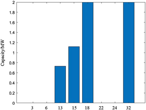
FIGURE 6. BESS allocation results of the proposed method.

TABLE 4

TABLE 4. Cost of DN with BESS.

Figure 7 shows the operation of DN with allocated BESS in typical scenarios. It can be seen that BESSs release energy for the growing loads in the morning. Then, with the increase in the PV power output and the decrease in load demand between 12:00 and 17:00, BESSs initiate charge to store the surplus energy. Then, during the peak load period, BESSs are discharged to support the high-load demand. Moreover, the energy trading power that reverse to the upper-level grid is significantly decreased during the peak PV period. Particularly, in scenarios 2 and 4, the reverse power reduces to 0, which illustrates that the installation of BESS can enhance the DN’s ability to harvest more renewable energy.

FIGURE 7

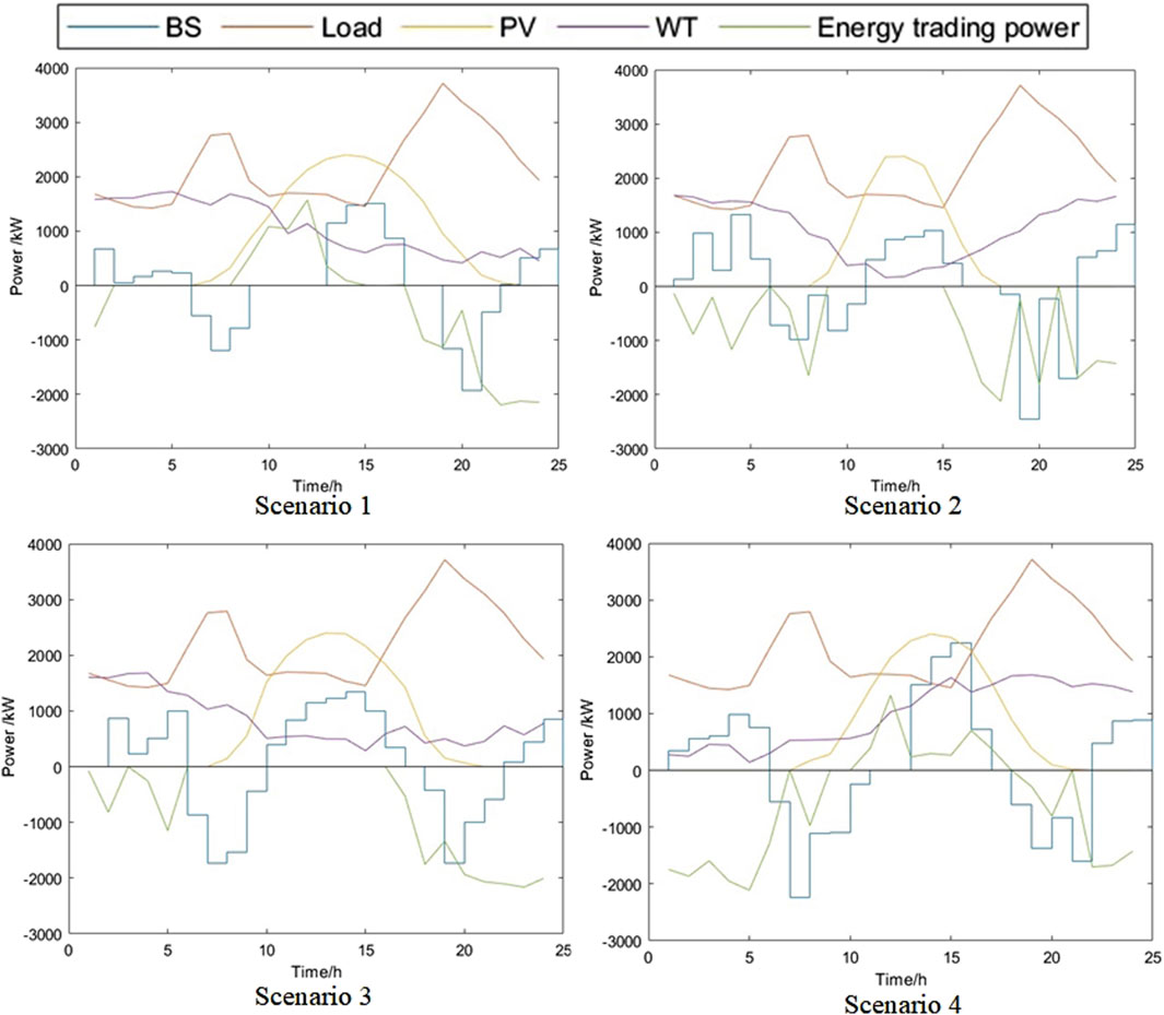
FIGURE 7. Charge/discharge situation of BESS in typical scenarios.

4.2.2 Comparison of the solution algorithm

The above BESS allocation model has numerous integer variables with a large number of optimization scenarios, which can easily lead to large solving time. This article solves the proposed allocation problem based on the FP algorithm to increase solving efficiency.

In order to verify the effectiveness of the proposed FP-based algorithm, another method that applies Gurobi solver to directly solve the proposed problem is used for comparison, and the solving results are shown in Table 5. Meanwhile, the convergence of the FP-based method is shown in Figure 8. It can be seen that using Gurobi solver to directly solve the proposed problem is difficult to converge because the planning problem contains a large number of 0–1 variables, and the problem dimension is high. By using the algorithm proposed above, mixed integer programming can be transformed into linear programming, greatly improving the single-solution speed. After testing, in this example, the proposed strategy can achieve convergence after six iterations, and the solver time of the proposed method is significantly decreased.

TABLE 5

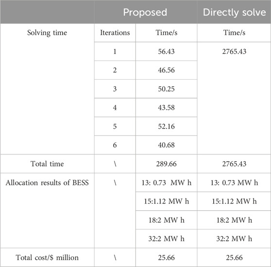
TABLE 5. Optimization result comparison.

FIGURE 8

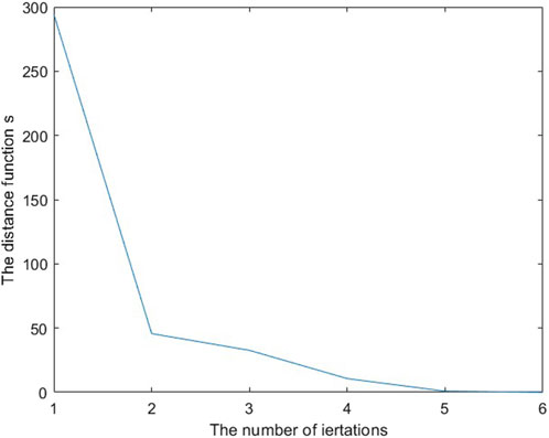
FIGURE 8. Convergence of the algorithm iteration.

4.2.3 Economy comparison

To analyze the economic performance of the proposed model, three BESS allocation methods are applied for comparison, which are given as follows:

Method A: A certain BESS allocation model without considering the uncertainties of RDGs and loads.

Method B: The BESS allocation model based on the RO method. The prediction intervals are set as ± 20% of the RDG output and ± 10% of the load output.

Then, 1,000 test scenarios are randomly generated based on the prediction bounds. Each scenario functions as a manifestation of uncertainty and undergoes testing in the three BESS allocation results. The expected total cost of the three methods is shown in Table 6.

TABLE 6

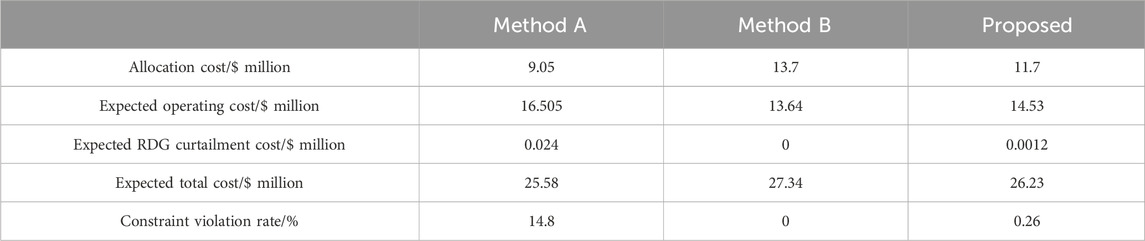
TABLE 6. Comparison of economic performance.

As shown in Table 6, since the results of Method B are obtained under the worst case, DN can achieve the safe operation and full RDG output consumption during testing, but the expected total cost is the highest among the three methods due to the highest installation cost of BESS. Additionally, both Method A and the proposed method all need to necessitate the use of an RDG power curtailment strategy to maintain the safe operation of DN. Moreover, in comparison to Method A, the proposed method demonstrates notably lower expected RDG curtailment costs and constraint violation rates. Thus, the proposed method has the ability to achieve the comprehensive optimal performance in terms of security and economic efficiency.

5 Conclusion

This paper proposes a stochastic optimal BESS allocation method, aiming to minimize the overall cost of DNs and prompt the renewable energy consumption. In this method, besides the stochastic nature of generation and demand, BESS degradation cost, capacity degradation, and the annual dynamic growth of generation and demand are also being considered. In addition, considering the proposed problem has massive integer variables, this paper is based on the FP algorithm to solve it. Based on the analysis of the allocation results, the following conclusion can be summarized:

1) In the comparison of the operating results in the proposed FP-based method and directly solving method, the proposed method can effectively mitigate the challenges posed by a high volume of integer variables, thereby improving the efficiency of solving the BESS allocation model.

2) The phenomenon of RDG curtailment has significantly decreased with the installation of BESS, which is important for the economic operation of DN.

3) The proposed method has the ability to achieve the comprehensive optimal performance in terms of security and economic efficiency.

However, current research primarily concentrates on the allocation of BESS and has not yet taken into account the influence of different regulating devices in DN. The future research work is devoted to investigating smart charge/discharge operations of BESS and the multi-time-scale coordinate allocation strategy, considering the operational characteristics of multiple regulating devices (such as capacitors and soft open points) in DN.

Data availability statement

The original contributions presented in the study are included in the article/Supplementary Material; further inquiries can be directed to the corresponding author.

Author contributions

CZ: conceptualization, methodology, and writing–review and editing. ZL: conceptualization, methodology, and writing–review and editing. LM: conceptualization, methodology, and writing–review and editing. SL: data curation and writing–original draft. LF: formal analysis, methodology, and writing–review and editing. HZ: formal analysis and writing–review and editing. HW: writing–original draft. YW: writing–original draft.

Funding

The author(s) declare that financial support was received for the research, authorship, and/or publication of this article. This study was supported by China Southern Power Grid Company Limited, Research on Key Technologies for Power Supply Guarantee of Mountain Power Grid Based on Microgrid (NO:070000KK52210030).

Conflict of interest

Authors CZ, ZL, LM, SL, LF, HZ, HW, and YW were employed by the Hainan Power Grid Co., Ltd.

Publisher’s note

All claims expressed in this article are solely those of the authors and do not necessarily represent those of their affiliated organizations, or those of the publisher, the editors, and the reviewers. Any product that may be evaluated in this article, or claim that may be made by its manufacturer, is not guaranteed or endorsed by the publisher.

References

Chen, J. (2023). Optimize configuration of multi-energy storage system in a standalone Microgrid. Front. Energy Res. 11. doi:10.3389/fenrg.2023.1283859

CrossRef Full Text | Google Scholar

Cheng, Y., Ye, S., Wang, R., Gao, H., and Liu, J. (2023). “Joint planning of electric vehicle charging station and energy storage system in the distribution network,” in 2023 Panda Forum on Power and Energy (PandaFPE), Chengdu, China, 30th April 2023, 225–230.

CrossRef Full Text | Google Scholar

Farzin, H., Fotuhi-Firuzabad, M., and Moeini-Aghtaie, M. (2016). A practical scheme to involve degradation cost of lithium-ion batteries in vehicle-to-grid applications. IEEE Trans. Softw. Eng. 7 (4), 1730–1738. doi:10.1109/tste.2016.2558500

CrossRef Full Text | Google Scholar

Fischetti, M., Glover, F., and Lodi, A. (2005). The feasibility pump. Math. Program. 104 (1), 91–104. doi:10.1007/s10107-004-0570-3

CrossRef Full Text | Google Scholar

Gräf, D., Marschewski, J., Ibing, L., Huckebrink, D., Fiebrandt, M., Hanau, G., et al. (2022). What drives capacity degradation in utility-scale battery energy storage systems? The impact of operating strategy and temperature in different grid applications. J. Energy Storage 47, 103533. doi:10.1016/j.est.2021.103533

CrossRef Full Text | Google Scholar

He, G., Chen, Q., Kang, C., Pinson, P., and Xia, Q. (2016). Optimal bidding strategy of battery storage in power markets considering performance-based regulation and battery cycle life. IEEE Trans. Smart Grid 7 (5), 2359–2367. doi:10.1109/tsg.2015.2424314

CrossRef Full Text | Google Scholar

Hidalgo-León, R., Siguenza, D., Sanchez, C., León, J., Jácome-Ruiz, P., Wu, J., et al. (2017). “A survey of battery energy storage system (BESS), applications and environmental impacts in power systems,” in 2017 IEEE Second Ecuador Technical Chapters Meeting (ETCM), Salinas, Ecuador, 16-20 October 2017, 1–6.

Google Scholar

Hua, H., Qin, Z., Qin, Y., Dong, N., Ye, M., Wang, Z., et al. (2022). Data-driven dynamical control for bottom-up energy Internet system. IEEE Trans. Sustain. Energy 13 (1), 315–327. doi:10.1109/tste.2021.3110294

CrossRef Full Text | Google Scholar

Huang, J., Wang, S., Xu, W., Fernandez, C., Fan, Y., and Chen, X. (2021). An improved rainflow algorithm combined with linear criterion for the accurate Li-ion battery residual life prediction. Int. J. Electrochem. Sci. 16 (7), 21075. doi:10.20964/2021.07.29

CrossRef Full Text | Google Scholar

Ju, C., Wang, P., Goel, L., and Xu, Y. (2018). A two-layer energy management system for microgrids with hybrid energy storage considering degradation costs. IEEE Trans. Smart Grid 9 (6), 6047–6057. doi:10.1109/tsg.2017.2703126

CrossRef Full Text | Google Scholar

Li, C., and Grossmann, I. E. (2021). A review of stochastic programming methods for optimization of process systems under uncertainty. Front. Chem. Eng. 2, 622241. doi:10.3389/fceng.2020.622241

CrossRef Full Text | Google Scholar

Li, C., Xu, Y., Yu, X., Ryan, C., and Huang, T. (2017). Risk-averse energy trading in multienergy microgrids: a two-stage stochastic game approach. IEEE Trans. Ind. Inf. 13 (5), 2620–2630. doi:10.1109/tii.2017.2739339

CrossRef Full Text | Google Scholar

Li, D., Wan, R., Xu, B., Yao, Y., Dong, N., and Zhang, X. (2023). Optimal capacity configuration of the wind-storage combined frequency regulation system considering secondary frequency drop. Front. Energy Res. 11, 1037587. doi:10.3389/fenrg.2023.1037587

CrossRef Full Text | Google Scholar

Meng, H., Jia, H., Xu, T., Wei, W., and Wang, X. (2023). Battery storage configuration of AC/DC hybrid distribution networks. CSEE J. Power Energy Syst. 9 (3). doi:10.17775/CSEEJPES.2021.07630

CrossRef Full Text | Google Scholar

Mohamad, F., Teh, J., and Lai, C.-M. (2021). Optimum allocation of battery energy storage systems for power grid enhanced with solar energy. Energy 223, 120105. doi:10.1016/j.energy.2021.120105

CrossRef Full Text | Google Scholar

Mohsenian-Rad, H. (2016). Optimal bidding, scheduling, and deployment of battery systems in California day-ahead energy market. IEEE Trans. Power Syst. 31 (1), 442–453. doi:10.1109/tpwrs.2015.2394355

CrossRef Full Text | Google Scholar

Mohseni-Bonab, S. M., Kamwa, I., Moeini, A., and Rabiee, A. (2020). Voltage security constrained stochastic programming model for day-ahead BESS schedule in Co-optimization of T&D systems. IEEE Trans. Sustain. Energy 11 (1), 391–404. doi:10.1109/tste.2019.2892024

CrossRef Full Text | Google Scholar

Ochoa-Barragán, R., Ponce-Ortega, M., and Tovar-Facio, J. (2023). Long-term energy transition planning: integrating battery system degradation and replacement for sustainable power systems. Sustain. Prod. Consum. 42, 335–350. doi:10.1016/j.spc.2023.09.017

CrossRef Full Text | Google Scholar

Pamshetti, V. B., and Singh, S. P. (2022). Coordinated allocation of BESS and SOP in high PV penetrated distribution network incorporating DR and CVR schemes. IEEE Syst. J. 16 (1), 420–430. doi:10.1109/jsyst.2020.3041013

CrossRef Full Text | Google Scholar

Schneider, S. F., Novák, P., and Kober, T. (2021). Rechargeable batteries for simultaneous demand peak shaving and price arbitrage business. IEEE Trans. Sustain. Energy 12 (1), 148–157. doi:10.1109/tste.2020.2988205

CrossRef Full Text | Google Scholar

Shao, Y., Ding, R., and Tian, Z. (2020). “An optimal configuration method for energy storage systems in distribution networks considering battery life,” in 2020 IEEE 3rd Student Conference on Electrical Machines and Systems (SCEMS), Jinan, China, 04-06 December 2020, 692–697.

CrossRef Full Text | Google Scholar

Taha, H. A., Alham, M. H., and Youssef, H. K. M. (2022). Multi-objective optimization for optimal allocation and coordination of wind and solar DGs, BESSs and capacitors in presence of demand response. IEEE Access 10, 16225–16241. doi:10.1109/access.2022.3149135

CrossRef Full Text | Google Scholar

Valentin, M., Julian, d. H., Marcus, B., Arun, V., and Shivkumar, K. (2015). “A multi-factor battery cycle life prediction methodology for optimal battery management,” in Proc. ACM 6th Int. Conf. Future Energy Syst., Bangalore, India, July 14-17, 2015, 57–66.

Google Scholar

Wang, B., Zhang, C., and Dong, Z. Y. (2020). Interval optimization based coordination of demand response and battery energy storage system considering SOC management in a Microgrid. IEEE Trans. Sustain. Energy 11 (4), 2922–2931. doi:10.1109/tste.2020.2982205

CrossRef Full Text | Google Scholar

Wang, B., Zhang, C., Dong, Z. Y., and Li, X. (2021). Improving hosting capacity of unbalanced distribution networks via robust allocation of battery energy storage systems. IEEE Trans. Power Syst. 36 (3), 2174–2185. doi:10.1109/tpwrs.2020.3029532

CrossRef Full Text | Google Scholar

Wang, B., Zhang, C., Li, C., Li, P., Dong, Z. Y., and Lu, J. (2022). Hybrid interval-robust adaptive battery energy storage system dispatch with SoC interval management for unbalanced microgrids. IEEE Trans. Sustain. Energy 13 (1), 44–55. doi:10.1109/tste.2021.3103444

CrossRef Full Text | Google Scholar

Xu, B., Oudalov, A., Andersson, A. G., and Kirschen, D. S. (2018a). Modeling of lithium-ion battery degradation for cell life assessment. IEEE Trans. Smart Grid 9 (2), 1131–1140. doi:10.1109/tsg.2016.2578950

CrossRef Full Text | Google Scholar

Xu, B., Oudalov, A., Ulbig, A., Andersson, G., and Kirschen, D. S. (2017). “Modeling of lithium-ion battery degradationfor cell life assessment,” in 2017 IEEE Power and Energy Society General Meeting, Chicago, IL, USA, 16-20 July 2017, 1.

CrossRef Full Text | Google Scholar

Xu, B., Zhao, J., Zheng, T., Litvinov, E., and Kirschen, D. S. (2018b). Factoring the cycle aging cost of batteries participating in electricity markets. IEEE Trans. Power Syst. 33 (2), 2248–2259. doi:10.1109/tpwrs.2017.2733339

CrossRef Full Text | Google Scholar

Yan, G., Liu, X., Yang, X., Chai, G., Guo, Q., and Gui, J. (2022). Combined source-storage-transmission planning considering the comprehensive incomes of energy storage system. Front. Energy Res. 10, 907338. doi:10.3389/fenrg.2022.907338

CrossRef Full Text | Google Scholar

Yang, Z., Hua, H., and Cao, J. (2023). Multiple impact factor based accuracy analysis for power quality disturbance detection. CSEE J. Power Energy Syst. 9 (1), 88–99. doi:10.17775/CSEEJPES.2020.01270

CrossRef Full Text | Google Scholar

Zhang, C., Dong, Z., and Yang, L. (2021b). A feasibility pump based solution algorithm for two-stage robust optimization with integer recourses of energy storage systems. IEEE Trans. Sustain. Energy. 12 (3), 1834–1837. doi:10.1109/tste.2021.3053143

CrossRef Full Text | Google Scholar

Zhang, W., and Wang, S. (2022). Optimal allocation of BESS in distribution network based on improved equilibrium optimizer. Front. Energy Res. 10, 936592. doi:10.3389/fenrg.2022.936592

CrossRef Full Text | Google Scholar

Zhang, Y., Kou, P., Zhang, Z., Tian, R., Yan, Y., and Liang, D. (2023a). Optimal sizing and siting of bess in high wind penetrated power systems: a strategy considering frequency and voltage control. IEEE Trans. Sustain. Energy 15, 642–657. doi:10.1109/tste.2023.3321302

CrossRef Full Text | Google Scholar

Zhang, Y., Su, Y., Chen, L., Liu, F., and Li, C. (2021a). “Robust allocation of battery energy storage considering battery cycle life,” in 2021 Power System and Green Energy Conference (PSGEC), Shanghai, China, May 13, 2021, 296–301.

CrossRef Full Text | Google Scholar

Zhang, Y., Xie, S., and Shu, S. (2023b). Decentralized optimization of multiarea interconnected traffic-power systems with wind power uncertainty. IEEE Trans. Industrial Inf. 19 (1), 133–143. doi:10.1109/tii.2022.3152815

CrossRef Full Text | Google Scholar

Zhao, L., Zeng, Y., Peng, D., and Li, Y. (2023). “Optimal economic allocation strategy for hybrid energy storage system under the requirement of wind power fluctuation,” in 2023 IEEE Power and Energy Society General Meeting (PESGM), Orlando, FL, USA, 16-20 July 2023, 1–5.

CrossRef Full Text | Google Scholar

Zheng, Y., Song, Y., Huang, A., and Hill, D. J. (2020). Hierarchical optimal allocation of battery energy storage systems for multiple services in distribution systems. IEEE Trans. Sustain. Energy 11 (3), 1911–1921. doi:10.1109/tste.2019.2946371

CrossRef Full Text | Google Scholar